


ABSTRACT
Known as the ‘Missing Baryon Problem’, about one-third of baryons in the local universe remain unaccounted for. The missing baryons are thought to reside in the warm–hot intergalactic medium (WHIM) of the cosmic web filaments, which are challenging to detect. Recent Chandra X-ray observations used a novel stacking analysis and detected an O vii absorption line towards the sightline of a luminous quasar, hinting that the missing baryons may reside in the WHIM. To explore how the properties of the O vii absorption line depend on feedback physics, we compare the observational results with predictions obtained from the Cosmology and Astrophysics with MachinE Learning (CAMEL) Simulation suite. CAMELS consists of cosmological simulations with state-of-the-art supernova (SN) and active galactic nuclei (AGNs) feedback models from the IllustrisTNG and SIMBA simulations, with varying strengths. We find that the simulated O vii column densities are higher in the outskirts of galaxies than in the large-scale WHIM, but they are consistently lower than those obtained in the Chandra observations, for all feedback runs. We establish that the O vii distribution is primarily sensitive to changes in the SN feedback prescription, whereas changes in the AGN feedback prescription have minimal impact. We also find significant differences in the O vii column densities between the IllustrisTNG and SIMBA runs. We conclude that the tension between the observed and simulated O vii column densities cannot be explained by the wide range of feedback models implemented in CAMELS.
1 INTRODUCTION
In the current standard Lambda cold dark matter (ΛCDM) cosmological model, baryons only make up a small part of the total energy and matter content of the Universe. Big bang nucleosynthesis (BBN; Cooke et al. 2014) and studies of the cosmic microwave background (CMB) have established the cosmic baryon mass density to be Ωb = 0.0449 (Planck Collaboration XIII 2016). Observations of distributions of galaxies in the local Universe also revealed a cosmic web pattern of the Universe’s large-scale structure (e.g. Geller & Huchra 1989), consistent with our current understanding of structure formation (e.g. Springel et al. 2005).
However, measurements of the baryon content of the local low-redshift z < 2 Universe do not corroborate with the BBN and CMB studies of the baryon budget. Only |$60\rm{-}$||$70\,\mathrm{per\,cent}$| of expected baryons have been uncovered (Shull, Smith & Danforth 2012). This is widely known as the ‘Missing Baryon Problem’ (Copi, Schramm & Turner 1995; Fukugita, Hogan & Peebles 1998; Burles, Nollett & Turner 2001; Bregman 2007).
Despite the challenges, there have been several attempts at detecting WHIM. Light from background quasars can be absorbed by the WHIM, producing absorption line features. Absorption lines of Ly α and O vi in the ultraviolet (UV) range have been detected around several quasars, providing evidence of the existence of the warm phases of the WHIM (e.g. Bahcall et al. 1993; Jannuzi et al. 1998; Tripp, Lu & Savage 1998; Tripp, Savage & Jenkins 2000; Lehner et al. 2007; Tripp et al. 2008; Stocke et al. 2014; Danforth et al. 2016). Because UV observations are only sensitive to the lower temperature WHIM, a substantial fraction of the hot (T > 105 K) phases of the WHIM remain undetected (Smith et al. 2011; Oppenheimer et al. 2012; Rahmati et al. 2016).
The bulk of the WHIM at higher temperatures is expected to emit weakly in the X-ray wavelengths. While X-ray emission has been detected from the hottest and highest density WHIM in the outskirts of galaxy clusters (Werner et al. 2008; Eckert et al. 2015; Alvarez et al. 2018; Tanimura et al. 2020), the density and gas temperature of the dominant fraction of the WHIM is too low to be detected in emission or individual absorption systems. Previous studies were highly controversial (Nicastro et al. 2005; Kaastra et al. 2006) and/or suffered from low detection significance (e.g. Mathur, Weinberg & Chen 2003), demonstrating the challenges of detecting WHIM. Some of the absorption signal may also come from within haloes of galaxies or galaxy groups instead of the large-scale WHIM (e.g. Nicastro et al. 2018; Johnson et al. 2019; Dorigo Jones et al. 2022). Additionally, these detections were obtained without a priori information of the redshifts of the detection, making it even more difficult to ascertain the origins of the detections as WHIM in the local Universe.
Recently, Kovács et al. (2019; hereafter K19) used 17 H i Lyman α absorbers with known redshifts that are associated with galaxies (Tripp et al. 1998) to enhance the signal-to-noise ratio of O vii absorption lines in the X-ray spectrum of the background quasar, H1821+643. This method used the redshifts of the H i absorbers to shift the O vii lines measured with Chandra/LETG to the rest frame. With the spectra shifted into the rest frame for each line, they were co-added to enhance the signal-to-noise ratio. This process revealed an O vii absorption line feature at a rest-frame wavelength of 21.6 Å, with a statistical significance of 3.3σ. A column density of NO vii = (1.4 ± 0.4) × 1015 cm−2 was computed, which is translated to an overall WHIM contribution of (37.5 ± 10.5) per cent to the total cosmic baryon mass density. To understand whether the O vii absorption line detected in K19 originates from the outskirts of galactic haloes or from the cosmic web filament, and how feedback from galaxies affect the WHIM signals, we compare the observational results with those predicted by cosmological simulations. To this end, we use the novel Cosmology and Astrophysics with MachinE Learning (CAMEL) simulation suite (Villaescusa-Navarro et al. 2022). The CAMEL simulation suite is a unique set of cosmological hydrodynamical simulations with varying supernovae (SN) and active galactic nuclei (AGNs) feedback. The CAMEL simulations use two galaxy formation hydrodynamic simulation codes as their fiducial models: IllustrisTNG (Nelson et al. 2018; Pillepich et al. 2018) and SIMBA (Davé et al. 2019), and then vary SN and AGN feedback prescriptions in a series of smaller volume simulations that allow one to examine how the parameter dependences of feedback physics impact the WHIM properties. We therefore aim to determine if a particular set of feedback parameters can recreate the purported K19 detection.
We organize the paper as follows. In Section 2, we give an overview of the CAMEL simulations, and also describe the methods for generating column densities, mocking ‘stacked’ column densities for comparison with K19, and our data analysis. We present our results in Section 3, with particular attention to splitting our sample based on distance to the nearest galaxy, as well as determining how the O vii column density strength relates to SN and AGN feedback. Finally, in Section 4 we give a summary and discussion of our results, as well as outline the next steps in the project.
2 METHODS
2.1 CAMEL simulations
The Cosmology and Astrophysics with MachinE Learning Simulations (CAMELS) data set (Villaescusa-Navarro et al. 2022) is a robust set of 4233 cosmological simulations, 2049 N-body, and 2184 hydrodynamical simulations. The simulations are based on a ΛCDM cosmological model and span a wide range of data objects ranging from galaxy haloes to spectra and radial profiles. All simulations consist of a |$(25 h^{-1}\mathrm{\, comoving\, Mpc})^3$| volume with base cosmological parameters Ωb = 0.049, h = 0.6711, and ns = 0.9624. The simulations are additionally based on the Illustris TNG and SIMBA simulation models, run using the arepo and gizmo codes, respectively; each of these models can be explored separately, as we do in this project. Additionally available in CAMELS are snapshots at redshifts ranging from z = 6 to z = 0, and we explore simulations at z = 0.154, to match the median redshift of the H i absorbers in K19. We use the 1P subset of CAMELS, a subset of 61 simulations that vary one cosmological or astrophysical parameter at a time across a range of 11 values (including the fiducial, or base case value) for each. These parameters include the cosmological parameters Ωm and σ8, and four astrophysical parameters, two corresponding to supernovae feedback and the other two to AGN feedback. We do not explore the effects of cosmology in this project, thus using a reduced 1P set. It is important to note that the SIMBA and IllustrisTNG simulations implement the astrophysical feedback differently. In addition, SIMBA tracks dust grains, and IllustrisTNG includes magnetohydrodynamics. The gravity and hydrodynamics solvers are different between the IllustrisTNG (Nelson et al. 2018; Pillepich et al. 2018) and SIMBA suites (Davé et al. 2019).
The four modes of SN and AGN feedback are parametrized as ASN1, ASN2, AAGN1, and AAGN2. In particular, the parameter ASN1 represents a normalization factor of the galactic wind feedback flux. This is implemented as either a pre-factor for the overall energy output per unit star formation (IllustrisTNG) or as a pre-factor for the wind mass outflow rate per unit SFR (SIMBA). As ASN2 represents the normalization factor for the galactic wind speed, varying ASN2 in IllustrisTNG maintains fixed energy output through adjustment of both wind speed and mass loading factor. In SIMBA, the mass loading factor stays fixed, and ASN2 varies the wind speed jointly with wind energy flux. As for the AGN parameters, AAGN1 is a normalization factor for the energy output of AGN feedback. In IllustrisTNG, this is implemented as the pre-factor power in kinetic feedback, while in SIMBA, AAGN1 is the pre-factor for the momentum flux of mechanical outflows in quasar and jet feedback. AAGN2 does not have a common definition across the two simulations but is defined as the parametrization of heated gas temperature and ‘burstiness’ in AGN bursts (IllustrisTNG) and an adjustment to the speed of continuously driven AGN jets (SIMBA). The ranges of variation for ASN1 and AAGN1 is [0.25, 4.0], while for ASN2 and AAGN2 it is [0.5, 2.0]. It is important to note that in contrast to the aforementioned astrophysical parameters, the cosmology parameter effects are designed to be the same across simulations.
2.2 2D CAMELS column density maps
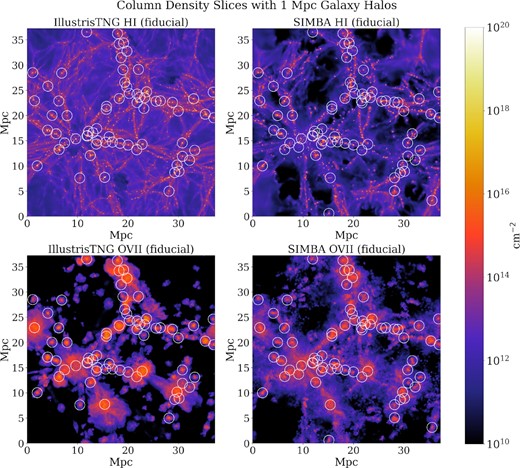
H i (top panels) and O vii (bottom panels) column density maps from the fiducial runs of the IllustrisTNG (left) and SIMBA (right) 1P simulation at z = 0.154 from a slice with width |$4.167\, h^{-1}$| Mpc. The colour indicates the value of the column density in units of cm−2. Overplotted are white 1 Mpc halo radii around galaxies in the simulation, which we define to be the halo outskirts of the galaxies. The haloes are selected to have virial masses Mvir ≥ 3 × 10¹¹ M⊙, and with their centres lying within the slice. Note that this visualization does not represent the methods of selecting regions for masked pixel maps described in Section 2.5.
When calculating the simulated column densities, we account for the main ionizing processes that determine the ionization balance for these two ions. Photoionization by the extragalactic ultraviolet background (UVB) radiation dominates for H i, while collisional ionization is dominant for O vii. We recalibrate the strength of the UVB to reproduce the observed statistics of the Lyman α Forest, which requires a UVB photoionization correction for each simulation run as described in Appendix A.
2.3 H i column densities from observation
| z | Equivalent width (mÅ) | 0.1 dex bin [|$\mathrm{log_{10}}(\mathrm{N_{H\,{\small I}}/\mathrm{cm^{-2}}})$|] |
|---|---|---|
| 0.05704 | 87 | 13.2 |
| 0.06432 | 62 | 13.0 |
| 0.08910 | 47 | 12.9 |
| 0.11152 | 66 | 13.0 |
| 0.11974 | 102 | 13.2 |
| 0.12157 | 353 | 13.8 |
| 0.12385 | 35 | 12.8 |
| 0.14760 | 229 | 13.6 |
| 0.16990 | 523 | 13.9 |
| 0.18049 | 75 | 13.1 |
| 0.19905 | 29 | 12.7 |
| 0.22489 | 739 | 14.1 |
| 0.24132 | 79 | 13.1 |
| 0.24514 | 79 | 13.1 |
| 0.25814 | 134 | 13.3 |
| 0.26156 | 163 | 13.4 |
| 0.26660 | 163 | 13.4 |
2.4 CDDF and stacking analysis
We calculate the O vii and H i Column Density Distribution Function (CDDF), defined as d2n/(dlog10Ndz) (where n is the number of absorbers and N is the column density), for the range of column density values log10(NO vii/cm−2) ∈ [5, 20] and log10(NH i/cm−2) ∈ [10, 25] with bin width of 0.1 dex, or 150 bins, which matches the precision of the observation in K19. We calculate n as the number of pixel counts in a 0.1 dex bin, dlog10N = 0.1, and with redshift path-length dz = 0.0015 (for a slice of full volume with dz = 0.0090), which we scale by the total number of pixels Npixel = 9.6 × 10⁷.
We then examine the CDDF of O vii at specific values of NH i corresponding to those of the 17 systems in the observation data in K19. Our 0.1 dex binning leads to duplicates in the H i column density values. For the 17 systems, there are 12 distinct values of NH i.
We also split the sightlines into two groups based on whether they were classified as corresponding to galaxy halo outskirts or cosmic web filament Lyman α absorbers in K19 (see Section 2.5 for more details on this separation criteria). This results in the total number of 15 distinct values of NH i, with 8 corresponding to the filamentary gas, and 7 for the extended halo regions. While there is overlap in the ranges of NH i values between these groups, we note that the highest values are in halo regions and the lowest are in filaments. This phenomenon is visible in Figs 2 and 4.

CDDFs for the binned NH i data in IllustrisTNG (top) and SIMBA (bottom) separated by the filament or halo outskirt pixel masking, based on the impact parameter b = 1 Mpc from galaxy haloes. The 50th (median) and 84th percentiles of these distributions are overplotted in dashed lines. From these results, we observe a slight shift in the medians, where the outskirt-only distributions have higher median NH i values. The distributions indicating the halo outskirts (b < 1 Mpc) are shifted towards higher NH i values than the filament (b > 1 Mpc) distributions, with smaller peaks in lower NH i regimes and a greater abundance in higher NH i values. These findings agree with our expectation that halo outskirt regions will contain more concentrated NH i than WHIM filaments. Additionally, we overplot the lines corresponding to H i absorbers in K19 (dotted), indicated by whether they are filament (orange) or halo outskirt (blue). The shift from the filament to halo outskirt here reflects the shift in the median. The K19NH i values are larger than the median of the IllustrisTNG distribution, and larger than the 84th percentile of the SIMBA distribution.

Distributions of log10(NO vii/cm−2) at each H i column density corresponding to the 8 filament H i absorbers and 7 halo outskirt H i absorbers from K19 for IllustrisTNG (left) and SIMBA (right) fiducial runs. The colour of the distribution line indicates the value of the log10(NH i/cm−2) sightline the O vii corresponds to, while the dashed lines indicate the K19 halo outskirt absorbers and solid lines indicate filament absorbers. Similarly, overplotted is the result from K19 (vertical, black dotted line). The higher NH i values correspond to lower counts of NO vii values, up until log10(NO vii/cm−2) ≈ 15, where the opposite becomes true. The distribution shapes between SIMBA and IllustrisTNG vary from one another, especially once this aforementioned threshold is crossed, with more high O vii values (log10(NO vii/cm−2) ≥ 16) being accounted for in IllustrisTNG than SIMBA.
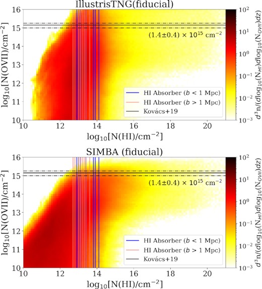
2D CDDFs for the log10(NH i/cm−2) plotted against log10(NO vii/cm−2) for IllustrisTNG (top) and SIMBA (bottom) fiducial runs. We simultaneously overplot the expected O vii column density from the observation result of (1.4 ± 0.4) × 1015 cm−2 (black) in K19, as well as vertical lines corresponding to the column densities of the H i absorbers (pink for filaments, blue for halo outskirts) with a bin size of 0.1 dex. Note that the heat map indicates the column density distribution function for the pixels in each bin. We observe that in the lower regime of column density values especially, the distributions look quite different between the two simulations. This is a consequence of the different feedback physics implementations of the two simulations. We focus more closely on the differences in the regime closer to the observed K19 O vii column density.
We then isolate NO vii distributions for each Lyman α absorber sightline at its corresponding NO vii bin and calculate the mean of each distribution as a proxy for the observed NO vii at each sightline. By averaging these values for a single simulation and feedback parameter, we can estimate the ‘stacked’ value of NO vii for that cosmology configuration.
2.5 Gas in outskirts of galactic haloes and in cosmic web filaments
The O vii column density (NO vii) can originate from WHIM in the cosmic web filament or gas in the outskirts of galaxy haloes. Physically, we expect the gas nearer to the haloes to be denser and more easily affected by the feedback process in the halo. Following K19, we split the absorbers into two samples based on their impact parameter from their nearest galaxies with Mvir ≥ 3 × 10¹¹ M⊙. Those with impact parameter less than b < 1 Mpc are referred to as ‘halo outskirts’, and those with b > 1 Mpc are referred to as ‘cosmic web filaments’. Note that we refrain from referring to the halo outskirt gas as the circumgalactic medium (CGM), as the CGM commonly refers to the gas within the virial radii of the galactic haloes, which in our case are smaller than 1 Mpc. Also note the parameter b = 1 Mpc criteria was chosen in K19 simply because it resulted in an approximately equal number of sightlines in both bins. To approximate the K19 cut, we use the coordinates for the galaxies in the fiducial simulations of SIMBA and IllustrisTNG and consider any projected absorber in the depth of the simulation volume within 1 Mpc as halo outskirt gas. K19 allowed velocity differences between the absorber and galaxy to exceed 1000 km s−1. Thus, we try to mimic this separation by allowing galaxies in all six of our slices to be associated with any absorber within 1 Mpc. The white circles in Fig. 1 indicate the 1 Mpc circular regions surrounding the galactic haloes for both IllustrisTNG and SIMBA fiducial runs. In most regions, the O vii absorbers with column densities log10(NO viI/cm−2) > 14 fall within 1 Mpc around galactic haloes. We apply these galaxy positions to other simulations with varied feedback parameters assuming that galaxies remain in roughly equivalent positions, even though their stellar masses change.
To more accurately explore true CGM regions, we modify the procedure above to select b < 300 kpc circular regions around galaxies with Mvir ≥ 3 × 10¹¹ M⊙ as ‘CGM’. For this selection, we also limit our galaxies by whether their central coordinates are located within a particular slice of the box, rather than looking at all galaxies within all six slices of the full box volume. We look at the full volume (six slices) to compile our statistics.
3 RESULTS
3.1 H i column density distributions
In Fig. 2, we show the CDDFs for the binned NH i data in SIMBA and IllustrisTNG for both filaments and halo outskirts. In units of log10(NH i/cm−2), the median H i CDDF of the filament component in SIMBA is 11.72, and 11.90 for the halo outskirt component; for the IllustrisTNG, the median H i CDDF for filament is 12.29, and for halo outskirt it is 12.48. This illustrates that the halo outskirts have higher median NH i than the filaments. This is in agreement with our expectation and the results from K19 that the denser halo outskirt regions contain more NH i absorbers than the filaments. It also shows that the IllustrisTNG predicts higher median NH i than SIMBA.
We also plot the H i column density values from the sightlines in K19 as vertical lines in Fig. 2. To have an appropriate comparison with K19, the sightlines in the simulations are selected using the same criteria in K19 (see Section 2.5). The K19 H i column densities are overall higher than the medians of the filament and halo outskirt distributions in the IllustrisTNG simulation and higher than the 84th percentile (roughly corresponding to 1σ above the median) in the SIMBA simulation. This suggests that the K19 sightlines are probing the denser parts of the filament and halo outskirts.
It may be unexpected that Figs 1 and 2 show such large differences between IllustrisTNG and SIMBA in the appearance and statistics of H i because both simulations have been normalized to the same UVB strength as described in Appendix A. The cosmic H i distribution is robustly reproduced by many hydrodynamic simulations at high redshift (Theuns et al. 1998; Davé et al. 1999; Altay et al. 2011; Rahmati et al. 2013). Part of the visual difference owes to the jet-mode AGN feedback in SIMBA travelling many virial radii and heating voids, leading to much lower column densities (Sorini et al. 2022; Tillman et al. 2022). AGN feedback is known to affect the H i column density statistics at low redshifts (Gurvich, Burkhart & Bird 2017; Burkhart et al. 2022). A detailed discussion of the differences between Simba and IllustrisTNG z = 0.1 H i column density distributions, and how different implementations of AGN feedback alter the H i distributions, can be found in Tillman et al. (2022). We further discuss the shape of the H i distribution in the Appendix, which is also different, as visible in Fig. 2.
3.2 O vii column density distributions
Fig. 3 shows the CDDFs of O vii for sightlines with the same H i column densities as in K19, for both fiducial runs of the IllustrisTNG and SIMBA simulations. Both simulations show more O vii absorbers for sightlines with lower NH i. The NO vii CDDF peaks at around log10(NO vii/cm−2) ≈ 12–14, where sightlines with higher NH i values peak at higher NO vii. Compared to the estimated log10(NO vii/cm−2) ≈ 15 from K19, the peaks of the NO vii values of the simulation are 1–2 orders of magnitude smaller.
There are significant differences in NO vii CDDF between IllustrisTNG and SIMBA. The peak in SIMBA occurs at lower NO vii, compared to IllustrisTNG. Thus, it is more unlikely to find O vii absorbers with the observed column density in the SIMBA runs. For the SIMBA runs, the distributions also drop sharply at log10(NO vii/cm−2) ≈ 15, whereas for IllustrisTNG, this drop-off varies with NH i. This drop-off occurs at higher NO vii for sightlines with higher NH i.
We also show the CDDFs separately for O vii in filaments and halo outskirts in both simulations. For a given NH i value, the halo outskirts tend to have slightly less O vii absorbers at low O vii column densities, but the trend is not significant.
In Fig. 4, we show the 2D CDDF d3n/(dlog NH idlog NO viidz) for both IllustrisTNG and SIMBA. For a given NH i value within the range of log10(NH i/cm−2) ∈ [12.7, 14.1], there is a very weak positive correlation between NO vii and NH i with large scatter. The correlation is slightly stronger in the SIMBA run compared to the IllustrisTNG run.
Fig. 5 shows the mean of the log10(NO vii/cm−2) distribution at given log10(NH i/cm−2) values that correspond to the K19 absorbers. It shows that means of the NO viI increase monotonically with NH i. In addition, we show separately the absorbers with impact parameter from their nearest galaxies b > 1 Mpc (solid squares) and b > 1 Mpc (empty circles). The b = 1 Mpc threshold is chosen to match with impact parameter binning in K19, which resulted in approximately the same number of absorbers in each bin (c.f. Section 2.5). Regardless of the impact parameter from the galaxies, the absorbers all follow the same monotonic trend. The IllustrisTNG values are consistently higher than the SIMBA values.

Comparison of the mean NO vii for different selection criteria for IllustrisTNG (blue) and SIMBA (orange) as a function of NH i. The solid lines indicate the mean μ of non-zero NO vii distributions at corresponding incremental 0.1 dex NH i values for 300 kpc CGM regions around galaxy halo locations. The dotted lines show the medians for these same 300 kpc distributions rounded to the nearest midpoint bin value. In the solid squares, we only present the average of the full O vii column density map at corresponding H i absorbers with an impact parameter b > 1 Mpc. In the empty circles, we show the average of the full O vii column density map at corresponding H i absorbers with an impact parameter b < 1 Mpc. There is overlap between these H i absorber separations. We show the median values of the full O vii column density maps at corresponding H i absorbers along the same division (× marker for b > 1 Mpc and + marker for b < 1 Mpc). Additionally, we observe that the average NO vii column densities for full maps fall much lower than the column densities for the 300 kpc CGM-only regions for both IllustrisTNG and SIMBA. That said, we see higher μ(NO vii) for IllustrisTNG than SIMBA throughout.
Note that b = 1 Mpc is much larger than the typical virial radius of the galaxies in the K19 sample. The true CGM is expected to be much closer to the galaxies. In the same figure we also show mean and median of NO vii as a function of NH i within b = 300 kpc of the simulated galaxies. At the same NH i, the mean NO vii values within 300 kpc are consistently higher by an order of magnitude than the halo outskirts and W hiM absorbers, for both IllustrisTNG and SIMBA, suggesting that the NO vii distribution at a given NH i is highly non-Gaussian, with a longer tail at the high end of NO vii.
3.3 Dependence of O vii column densities on feedback physics
Fig. 6 shows the estimated O vii column densities at each observed H i sightline across all values of the CAMELS feedback parameters presented in Section 2.2. We note that for all ranges of feedback parameters, the O vii column densities are still more than a magnitude below the observed estimates in K19, indicating that the differences we see between simulations and observations are unlikely due to feedback physics. Below, we examine in detail how the O vii column density depends on each CAMELS feedback mode.
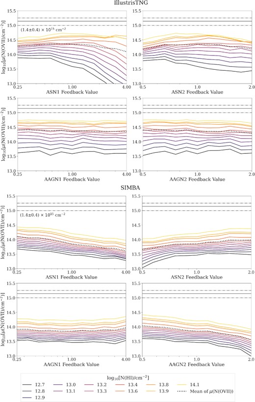
Dependence of feedback on the O vii column densities measured at the values of observed H i column densities. The top 4 panels show the results for the IllustrisTNG runs, while the bottom 4 show the SIMBA results. In each panel, the horizontal solid and dotted–dashed lines show, respectively, the mean and 1σ scatter of the observed NO vii value from K19. The coloured lines show the means of the NO vii distributions from the simulation for each observed NH i value, with the colours indicating the relative level of NH i. The dotted line shows the mean of the simulated NO vii estimates across all H i sightlines. It shows that NO vii is most dependent on varying SN1 and SN2 feedback in IllustrisTNG (SN energy per unit stellar mass and SN wind speed, respectively). More SN energy per stellar mass results in lower NO vii, especially for lower NH i values. Varying AGN feedback in IllustrisTNG has virtually no impact on NO vii. For SIMBA, all feedback modes except AGN1 (momentum flux of AGN outflow) result in changes in NO vii, though the dependences are quite weak. For all ranges of feedback parameters explored, none produce high enough NO vii to be consistent with observed value in K19.
3.3.1 Dependence on SN Feedback
The top left panel in Fig. 6 shows the estimated O vii column densities at each observed H i sightline across all values of ASN1 feedback for both IllustrisTNG and SIMBA simulations. In IllustrisTNG, the ASN1 represents the amount of energy in the SN feedback per unit stellar mass, and in SIMBA, it represents the mass loading factor. The O vii column density in both IllustrisTNG and SIMBA depends on this ASN1 parameter. To show that, we plot the ‘stacked’, or mean of means estimate of log10(NO vii/cm−2) at the observed NH i values. Increasing ASN1 feedback decreases the estimated O vii column densities for all H i sightlines in the SIMBA runs, and for H i sightline column densities log10(NH i/cm−2) ≲ 13.6 for the IllustrisTNG run. We interpret this trend as stronger suppression of star formation with increasing SN energy output, leading to lower oxygen yields and O vii. This effect is smaller at higher NH i in more massive haloes in IllustrisTNG, where SN feedback is less effective in quenching star formation.
We also examine the dependence on ASN2, representing the wind speed of SN feedback for both IllustrisTNG and SIMBA. Again, the ‘stacked’ value of O vii column density is lower than the value in K19 in all IllustrisTNG and SIMBA runs. In IllustrisTNG, we observe a slight decrease in O vii for log10(NH i/cm−2) ≲ 13.6, and a decrease in the remaining sightlines starting at ASN2 ≈ 1. In SIMBA, we see an increase in O vii as feedback increases across all sightlines, though this trend is not strictly monotonic, especially for H i absorbers with low column densities. In IllustrisTNG, the H i absorber sightlines that are most affected by the feedback fall into the regime of the filament rather than the halo outskirt, indicating that the halo outskirt may be more resilient to varying SN wind speed and mass loading factor. In SIMBA, both the halo outskirt and filament regimes appear to be affected by wind speed and wind energy flux modulation, though not uniformly.
3.3.2 Dependence on AGN Feedback
The AAGN1 feedback represents the energy of the AGN kinetic feedback in the IllustrisTNG runs and the momentum flux of the AGN outflow in the SIMBA runs. For AAGN1 feedback, we observe negligible effects of varied feedback for both simulation suites. For IllustrisTNG, there are no clear trends, suggesting that the kinetic feedback power adjustment has a limited impact on the O vii and H i column density distributions. For SIMBA, there is a small increase for the most extreme feedback values AAGN1 ≳ 3, but otherwise, the effect of quasar and jet outflows is negligible.
The AAGN2 feedback represents the temperature of the gas heated by each AGN outburst for IllustrisTNG and the speed of the jet outflow in the SIMBA runs. Because of the difference in the physical meaning of AAGN2 between the two suites, we see significant differences in the NO vii distributions between the two. For IllustrisTNG, there is a very slight decrease in NO vii as AAGN2 increases, especially at higher H i absorber sightline values (log10(NH i/cm−2) ≳ 13.1) and for stronger feedbacks (AAGN1 ≳ 1). For SIMBA, AAGN2 more strongly decreases O viI for all sightlines as feedback increases. We interpret this result as the O vii being more responsive to the speed of continuously driven AGN jets, where faster jets quench more star formation and thus inhibit O vii formation.
3.3.3 Origin of the dependence on feedback
The different dependence of NO viI mainly comes through the dependence of star formation quenching on feedback implementations. In Fig. 7, we show the distributions of the column densities of all oxygen species for the extreme runs of the 4 feedback modes for both IllustrisTNG and SIMBA. For the IllustrisTNG run, the oxygen column density distributions are sensitive to SN1 and SN2 feedback, representing the SN energy per unit stellar mass and the SN wind speed, respectively, while insensitive to AGN feedback. For the SIMBA runs, all SN and AGN feedback modes have considerable impact on the NO distribution at low column densities (for log10(NO/cm−2) < 15, but minimal impact otherwise.

Distributions of oxygen column densities NO for the IllustrisTNG (top panels) and SIMBA (bottom panels) runs. The left-hand panels show the distributions for min and max SN1 and SN2 runs. The right-hand panels show the distributions for min and max AGN1 and AGN2 runs. The figure shows that for the IllustrisTNG run, the oxygen column density distributions are most sensitive to varying the ASN1 and ASN2 parameters, which represent the SN energy per unit stellar mass and the SN wind speed, respectively. The NO distribution is insensitive to AGN feedback. On the other hand, for the SIMBA runs, all SN and AGN feedback modes have a considerable impact on the NO distribution at low column densities (for log10(NO/cm−2) < 15). The dependence on SN and AGN feedback in NO for both IllustrisTNG and SIMBA is similar to that of NO VII, suggesting that feedback does very little in changing the ionization state of oxygen. The dependence on feedback in NO vii is likely due to the suppression of star formation and hence total oxygen production.
The column densities of total oxygen O show the same qualitative dependence on feedback as that for O vii. This can be explained by the reduction in the production of metals in runs with stronger SN feedback, as the star formation and thus metal production is quenched more strongly, reducing the total amount of oxygen and its ionized species. In Fig. 8, we show the dependence of total stellar mass produced in the box on the strengths of the 4 feedback modes. For IllustrisTNG, the stellar mass is most sensitive to SN1 and SN2 feedback, but almost insensitive to AGN1 and AGN2 feedback. For SIMBA, increasing SN1 and SN2 feedback leads to mildly increasing and decreasing stellar mass, respectively; increasing both AGN1 and AGN2 feedback leads to a modest drop in stellar mass. These trends are consistent with the feedback dependence of NO in Fig. 7. The similar dependence of feedback in O, O viI (and stellar mass) implies that feedback has a limited impact on the ionization state of oxygen in W hiM.
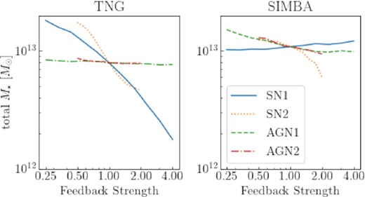
We show the total stellar mass at z = 0.154 produced in the CAMEL simulation box and its dependence on the feedback strengths, for both the IllustrisTNG runs (left-hand panel) and the SIMBA runs (right-hand panel). For TNG, the increasing ASN1 (blue line) and ASN2 (orange dotted line) decreases the total stellar mass, while increasing AAGN1 (green dashed ine) and AAGN2 (red dashed–dotted line) results in almost no change in stellar mass. On the contrary, for the SIMBA runs, increasing ASN1 leads to slight increase in stellar mass, while increasing the other feedback parameters leads to lower stellar mass.
Note that the O column density distribution also behaves quite differently between the IllustrisTNG and the SIMBA runs. First, the IllustrisTNG distribution has lower column density absorbers than SIMBA, for all feedback runs. Secondly, the column density distributions are more sensitive to SN feedback in the SIMBA runs than in the IllustrisTNG runs, especially at the lower column densities. This highlights the differences in the sub-grid modelling of feedback between IllustrisTNG and SIMBA and their predictions on WHIM properties.
4 CONCLUSIONS AND DISCUSSION
Using the CAMEL simulation suite, we study the O vii primarily arising from the Warm Hot Intergalactic Medium (WHIM), how this ion depends on feedback by SN and AGNs, and whether these simulations can reproduce the observed O vii X-ray absorption signal detected along the H1821+643 quasar sight line obtained by stacking known H i absorbers (Kovács et al. 2019,K19). Here are our main findings:
For all ranges of SN and AGN feedback parameters in CAMELS, the NO vii values for the WHIM are 1–2 orders of magnitude below the Chandra observation of NO vii in (Kovács et al. 2019, K19). In particular, the maximum value of NO vii is below NO vii of |$(1.4 \pm 0.4) \times 10^{15}\, \mathrm{cm^{-2}}$|, the observed value (see Fig. 6).
The O vii column density is most sensitive to the energy of the SN feedback per unit stellar mass in the IllustrisTNG runs, and the SN mass loading factor in SIMBA. Other modes of SN feedback and most AGN feedback explored in the CAMEL simualtion suite do little to affect O vii column density.
The O vii column density is insensitive to the AGN feedback energy in both IllustrisTNG and SIMBA, which can be attributed to the relative spatial rarity of AGNs relative to the stellar sources of SN feedback. On the other hand, increasing the AGN jet speed in the SIMBA runs lowers O vii, indicating these jets can impact a significant cosmic volume.
The relationship of O vii–H i column densities follows a similar relationship if found inside or outside a 1-Mpc radius from galaxies, in agreement with K19. This owes to the O vii arising almost entirely from the WHIM. In contrast, the CGM within 300 kpc of galaxies shows significantly stronger O vii for a given H i absorption strength, but this is not a dominant contribution to the H1821+643 sightline (see Figs 1 and 5).
The K19 estimate on the O vii column densities inferred from stacking of X-ray absorption lines is higher than nearly all of the sightlines in the CAMEL simulations with varying feedback physics for similar values of H i column densities as in the observation. In addition, in the simulation, not any one slightline dominates the average O vii column density estimate. In Appendix B, we show that the differences between simulations and observations are unlikely due to cosmic variance since going to a large simulation box will only explain 0.2 dex differences in the O vii column densities.
This suggests a tension between the observed O vii column density estimate in K19 and predictions from our simulations. This can mean either (1) the gas physics models adopted in both IllustrisTNG and SIMBA are insufficient to produce enough oxygen column densities, or (2) the K19 observed column density is dominated by a few strong absorbers that skew the stacked measurement towards high column densities, since individual absorbers were not detected. Exploring other astrophysical processes not varied in CAMELS, such as turbulent mixing, or stellar yield, may help distinguish between these two scenarios. Additionally, studying more sightlines will also help to resolve whether the H1821+643 sightline is brighter than other sightlines. To this end, we analyse additional sightlines based on Chandra archival observations in a follow-up study and compare the O vii column densities and upper limits with those observed in Kovács et al. (2019). The detailed comparison between the observed sightlines will be presented in an upcoming study.
We see that supernovae feedback typically affects the O vii distributions more than AGN feedback. This is because (1) supernovae feedback sources are more widely distributed than AGN sources, which are typically centred on rare, massive haloes, and (2) supernovae are more effective in suppressing star formation in the more abundant, lower mass haloes. Lower NO vii corresponding to lower NH i sightlines are more affected by the ASN1 feedback since these NO vii values reside in the more sparse filamentary structures, rather than the high NO vii, which are clustered around massive haloes. A larger simulation box with more massive, group-size haloes will allow us better to assess the impact of AGN feedback on WHIM.
The differences in the column density distributions between IllustrisTNG and SIMBA within CAMELS highlight that the feedback physics implementations have not yet converged. Both produce quite different O vii column density distributions despite having similar strengths of the feedback parameter. Specifically, the SIMBA runs generate consistently lower numbers of O vii absorbers at high column densities than IllustrisTNG. This suggests that the jet feedback in SIMBA runs (compared to kinetic feedback in IllustrisTNG) is more efficient in suppressing the production of stars and oxygen in more massive haloes. This also suggests that the relationship between O vii and H i column densities in the WHIM are sensitive to, and thus can be used to constrain feedback physics.
Ongoing analysis of Chandra observation of similar systems, but with deeper exposure, will help in resolving the differences in O vii column densities between simulation and observation. Future X-ray instruments with high spectral resolution and sensitivity, such as an ARCUS-like (Smith 2020) mission dedicated to X-ray absorption, the Athena X-Ray Observatory (Nandra et al. 2013), and the proposed Line Emission Mapper (LEM),1 can provide more accurate measurements of absorption line spectra (for WHIM emission, see Parimbelli et al. 2022 for CAMELS prediction for Athena), all necessary for uncovering a more realistic picture of the complex gas structures present in the universe and the locations of elusive low-redshift baryons.
ACKNOWLEDGEMENTS
We thank the anonymous referee whose comments improve the presentation of the paper. We also Nastasha Wijers, Joop Schaye, and Johnny Dorigo Jones for their comments. We gratefully acknowledge the CAMELS team for publicly releasing CAMELS data. We also acknowledge the Center for Computational Astrophysics at the Flatiron Institute for providing the computing facilities for making the CAMELS maps and the Yale Center for Research Computing for enabling our use of High-Performance Computing. This work is supported by NSF grant AST-2206055. ÁB acknowledges support from the Smithsonian Institution and the Chandra High Resolution Camera Project through NASA contract NAS8-03060. OEK is supported by the GACR grant 21-13491X.
DATA AVAILABILITY
The instructions for accessing the CAMELS data (Villaescusa-Navarro et al. 2022) can be found here: https://camels.readthedocs.io/en/latest/data_access.html. Accessing the Trident code suite (Hummels et al. 2017) to enable manipulation and analysis of CAMELS data can be found here: https://trident.readthedocs.io/en/latest/.
Footnotes
REFERENCES
APPENDIX A: H I PHOTOIONIZATION CORRECTION
The photoionization corrections are found using the code that generated the Lyman α spectra released with the CAMELS public data release (Villaescusa-Navarro et al. 2022). The spectra were generated using the publicly available code outlined in Bird et al. (2015) and Bird (2017).2 Utilizing addition code from the ‘fake spectra’ package, we can calculate UVB corrections. We recalculate the temperature and electron abundance given a photocorrection factor with the hydrogen and helium photoionizing and photoheating values and the appropriate recombination values. By solving the ionization equilibrium equation, we can find the corrected neutral hydrogen fraction and generate new UVB corrected Lyman α spectra.
To find the UVB correction factors used in this study, we fit the new corrected Lyman α spectra to the observed Danforth et al. (2016) CDDF data. We fit a range of UVB correction factors using a simple χ2 reduction method. The CDDFs generated from these spectra files are calculated similarly to the method outlined in Burkhart et al. (2022). We find these CDDFs by direct integration rather than through Voigt fitting.
We refer the reader to Tillman et al. (2022) for more details on the comparison of feedback models in cosmological simulations on H i column densities.
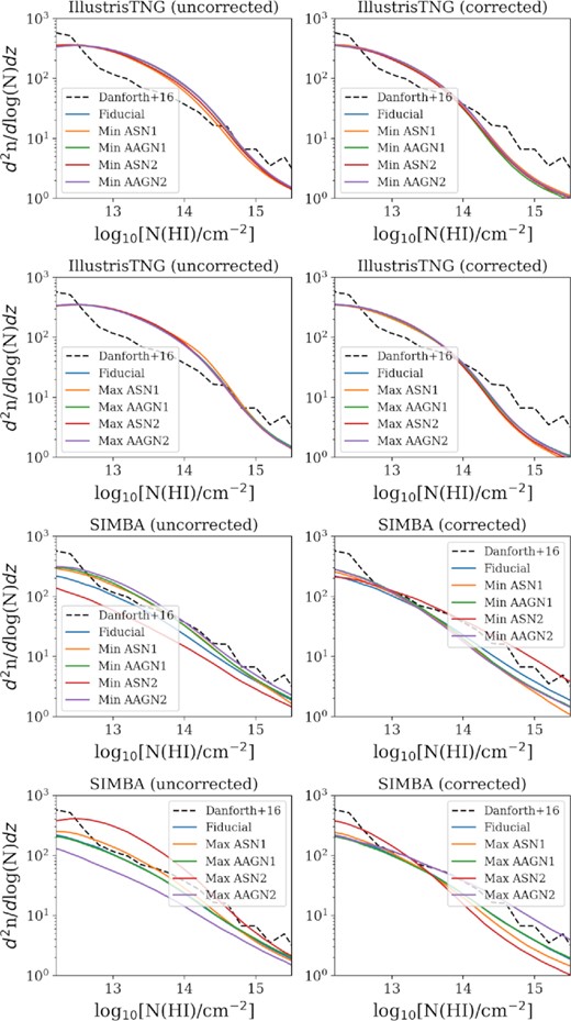
CDDFs of H i in the CAMEL simulations. The top four panels show the H i CDDFs of the IllustrisTNG and SIMBA runs with minimum and maximum feedback values for the original simulation outputs. The bottom four show similar plots for the Illustris and SIMBA runs but renormalized using corrections from UV photoionization, which are detailed in Tillman et al. (2022). The dashed lines indicate the observations from Danforth et al. (2016).
APPENDIX B: BOX SIZE AND RESOLUTION CONVERGENCE
Although the CAMEL simulations do not have other box sizes and resolutions, we can use results from previous work to estimate the effects of changing both. For box size, Wijers et al. (2019) explored EAGLE simulations (Crain et al. 2015; Schaye et al. 2015) with box sizes from 25 to 100 comoving Mpc on a side. They found deviations of up to 0.2 dexes higher below NO VII = 1016 cm−2 for a 25 Mpc volume compared to the main 100 Mpc volume, which is the primary EAGLE simulation and contains 64 × more volume than the 25 Mpc volume. The CAMELS volumes, at 37.25 Mpc, contain 19 × less volume than the primary EAGLE simulation and fall between the 25 and 50 Mpc volumes shown in fig. A3 of Wijers et al. (2019). The 50 Mpc EAGLE volume shows much better convergence than the 100 Mpc volume, suggesting that the box size effect is an ∼0.1–0.2 dex change at most.
As for resolution convergence, Wijers et al. (2019) explore a factor of 8 × higher mass resolution showing better than 0.1 dex convergence below NO vii = 1015.5 cm−2. However, the CAMELS gas fluid element resolution is 1.89 × 10⁷M⊙, which is 10 × lower than the EAGLE resolution. Therefore, we consider the IllustrisTNG100-2 simulation with a mass resolution of 1.1 × 10⁷ M⊙ (Nelson et al. 2019). Nelson et al. (2018) demonstrated this simulation’s NO vii CDDF is converged to within within 0.1 dex of the 8 × better resolution IllustrisTNG100-1 simulation. While this is a lower oxygen species, we expect the 0.1 dex resolution convergence to be a good indicator for O vii. The CAMELS’ smaller box size and lower resolution than other published results from the larger and higher resolution EAGLE and IllustrisTNG main simulation runs suggest that O vii will not change by more than 0.2 dex, which cannot make up for the shortfall compared to the K19 observation.
