


ABSTRACT
We examine the H i gas kinematics of galaxy pairs in two clusters and a group using Australian Square Kilometre Array Pathfinder (ASKAP) WALLABY pilot survey observations. We compare the H i properties of galaxy pair candidates in the Hydra I and Norma clusters, and the NGC 4636 group, with those of non-paired control galaxies selected in the same fields. We perform H i profile decomposition of the sample galaxies using a tool, baygaud, which allows us to deblend a line-of-sight velocity profile with an optimal number of Gaussian components. We construct H i superprofiles of the sample galaxies via stacking of their line profiles after aligning the central velocities. We fit a double Gaussian model to the superprofiles and classify them as kinematically narrow and broad components with respect to their velocity dispersions. Additionally, we investigate the gravitational instability of H i gas discs of the sample galaxies using Toomre Q parameters and H i morphological disturbances. We investigate the effect of the cluster environment on the H i properties of galaxy pairs by dividing the cluster environment into three subcluster regions (i.e. outskirts, infalling, and central regions). We find that the denser cluster environment (i.e. infalling and central regions) is likely to impact the H i gas properties of galaxies in a way of decreasing the amplitude of the kinematically narrow H i gas (|$M_{\rm {narrow}}^{\rm {H\, \small {\rm I}}}$|/|$M_{\rm {total}}^{\rm {H\, \small {\rm I}}}$|), and increasing the Toomre Q values of the infalling and central galaxies. This tendency is likely to be more enhanced for galaxy pairs in the cluster environment.
1 INTRODUCTION
According to the Λ Cold Dark Matter hierarchical structure formation of galaxies, galaxy mergers and tidal interactions are critical for regulating the star formation (SF) histories of galaxies over cosmic time. Mergers and tidal interaction can lead to either enhancing or quenching of their SF (Mihos & Hernquist 1996; Di Matteo et al. 2007; Ellison et al. 2013; Patton et al. 2013; Ellison, Catinella & Cortese 2018; Quai et al. 2021). The effective angular momentum transport outwards and the subsequent gas funneling inwards caused by the mergers and tidal interactions of galaxies can boost the creation of giant molecular gas clouds and thus SF in galaxies (Mihos & Hernquist 1996; Di Matteo et al. 2007). On the other hand, the merging process can also give rise to turbulent gas motions that can suppress SF (Ellison et al. 2018; van de Voort et al. 2018). It is important to examine how the merging process affects the gas properties of galaxies, as this will lead us towards a better understanding of SF and the resulting galaxy evolutionary path.
Galaxy clusters are the largest known gravitationally bound systems and typically contain hundreds or thousands of galaxies, larger than galaxy groups which are also gravitationally bound objects, but generally contain fewer galaxies. Galaxy clusters provide a high galaxy number density environment analogous to the early Universe where more frequent galaxy interactions are expected than in the local Universe. Many studies have discussed the effect of galaxy interactions in the cluster environment on their physical properties such as SF rate, metallicity, colours, luminosity, morphology, and gas properties (Alonso et al. 2004, 2012; Park & Hwang 2009; Ellison et al. 2010; Oh et al. 2019b; Cortese, Catinella & Smith 2021).
An area of particular interest has been to examine how the merging process in cluster environments affects both molecular and atomic gas properties in and around galaxies: (1) How much of the cool gas reservoir is used up or replenished during galaxy mergers? (Georgakakis, Forbes & Norris 2000; Yamashita et al. 2017); (2) How are the fractions of gas in different phases (atomic, molecular, and ionized) changed in the course of galaxy merger sequence, and how do they relate to SF processes? (Georgakakis et al. 2000; Moreno et al. 2021); (3) Which fuelling mechanism, such as cool gas accretion from interacting galaxies or gas replenishment from the cooling of ionized gas in haloes, is dominant during the galaxy merger? (Moster et al. 2011; Ellison, Patton & Hickox 2015b); (4) How can one distinguish between the effects of ram pressure stripping and tidal interaction on the gas properties of galaxies in a cluster environment, and which effect would prevail under what conditions? (Mihos 2003; Yoon et al. 2017). Recent studies of merging or interacting galaxies find an agreement between observed and simulated gas properties: the triggered nuclear SF, enhanced molecular gas fractions (MH2/M*), and higher SF efficiency (SFE) compared to non-paired galaxies (Ellison et al. 2013; Michiyama et al. 2016; Pan et al. 2018; Violino et al. 2018).
Close galaxy pairs, also known as pre-merger galaxies, are in close proximity and have similar line-of-sight velocities. These close pairs provide crucial information about how galaxy interactions affect gas properties and SF in the early phase of a merger sequence. High-resolution, parsec-scale galaxy merger simulations show that the majority of close encounters experience centrally concentrated and enhanced SF that is mainly driven by cold gas inflow (Patton et al. 2020; Moreno et al. 2021), whilst there are cases where SF in the central and outer regions of galaxies is suppressed by the reduced SFE. Hydrodynamical effects that drive turbulent gas motions such as stellar feedback and gravitational interactions can decrease SFE in galaxy pairs (Moreno et al. 2021).
H i in close galaxy pairs can be used for probing the environmental effect on the physical conditions of the cool gas reservoir. H i is particularly useful for investigating the gas physics of galaxy pairs in the early phases of interaction, as it is the most sensitive constituent of the system to any gravitational distortions. In addition, the dynamical time-scale on which H i gas reacts to external influences is relatively shorter than that of other constituents in the galaxy pairs, like stars.
Several studies have performed H i observations of galaxy pairs in order to investigate the effect of gravitational interactions between them on their cool gas properties (e.g. Zuo et al. 2018). These include the ALFALFA1 studies which discuss H i gas fraction offsets of post-merger galaxies relative to isolated control galaxies (Ellison et al. 2015a). However, these observations lack spatial resolution due to the single dishes’ beam resolutions that are not high enough to resolve the internal gas kinematics and H i distribution of close galaxy pairs.
H i interferometric observations were carried out for a few tens of galaxy pairs but their beam resolutions were not high enough to spatially resolve individual galaxies given their distance (Scudder et al. 2015). There was limited information about their spatially resolved kinematics (e.g. rotation curve analysis). To date, high-resolution H i interferometric observations for a significant number of close galaxy pairs are limited (Nordgren et al. 1997a; Nordgren et al. 1997b; Koribalski & López-Sánchez 2009). An important step towards a better understanding of the cool H i gas properties of galaxy pairs is to obtain information about the spatially resolved H i distribution and kinematics for a larger sample.
In this paper, we examine the resolved H i gas properties of close galaxy pairs in two galaxy clusters (Hydra I and Norma), and a galaxy group (NGC 4636) from the Widefield Australian Square Kilometre Array Pathfinder (ASKAP) L-band Legacy All-sky Blind surveY (WALLABY) pilot observations undertaken with the ASKAP. WALLABY is an ASKAP all-sky H i galaxy survey that is expected to detect ∼210 000 galaxies out to z ∼0.1 (Koribalski et al. 2020; Westmeier et al. 2022). WALLABY pilot observations provide high-quality H i 21 cm data of resolved galaxies in the two galaxy clusters and the galaxy group with an angular resolution of 30 arcsec at an rms of 2.0 mJy beam−1 per 4 |$\mathrm{km}\, \mathrm{s}^{-1}$| channel spacing. The 30-square-degrees of ASKAP’s wide field of view makes it possible to efficiently map the H i emission over the large area of sky. Given the distances to these galaxy clusters and the group, H i gas discs of more than 90|${{\ \rm per\ cent}}$| of member galaxies are marginally resolved, more than three beams across their major axes.
We perform profile decomposition of H i velocity profiles using a new tool, baygaud. This new software allows us to deblend a line-of-sight velocity profile with an optimal number of Gaussian components based on Bayesian analysis techniques (Oh, Staveley-Smith & For 2019a; Oh et al. 2022; Park et al. 2022). We construct an H i superprofile of each galaxy via stacking of individual line profiles after aligning their central velocities. We then fit a double Gaussian model to the H i superprofile and classify them as the kinematically narrow and broad H i gas components with respect to their velocity dispersions, respectively. From this, we aim to investigate how the H i gas in different kinematic phases (i.e. the narrow and broad components) are affected by the merging process in different galaxy environments. Practically, we examine the variations of not only small-scale H i kinematics but also the kinematically cool-to-total H i mass ratios of galaxy pairs at their fixed total H i masses in cluster environments. Additionally, we quantify the gravitational instability of the gas discs of galaxy pairs against gas collapse and SF by deriving their Toomre Q parameters (Toomre 1964). We also measure morphological H i asymmetries to quantify the gas discs’ disturbances. Galaxy pairs are classified as outskirts, infalling, and central ones based on the locations of the phase-space diagrams of the clusters and the group.
This paper is organized as follows. In Section 2, we present our data and perform a classification of galaxy pairs and non-paired galaxies. In Section 3, we derive the H i properties of the sample galaxies. In Section 4, we investigate the effect of the cluster environment on the H i gas in the phase-space diagram of the galaxy clusters and group. Lastly, we summarize the main results of this paper in Section 5. Throughout this paper, we adopt the Hubble constant H0 as 70 |$\mathrm{km}\, \mathrm{s}^{-1}$| Mpc−1.
2 DATA
2.1 ASKAP H i 21 cm pilot observations
In order to investigate the resolved H i gas properties of galaxy pairs in the cluster and group environments, we use the H i 21 cm line data of two galaxy clusters, Hydra I and Norma, and a galaxy group, NGC 4636 taken from the ASKAP pilot observations. Prior to the start of the full survey, three 60-square-degree fields in the direction of the Hydra I cluster, Norma cluster, and NGC 4636 group were observed during the ASKAP pilot survey phase. ASKAP pilot observations with 36 × 12 m dishes at a channel resolution of 4 |$\mathrm{km}\, \mathrm{s}^{-1}$| and a beam resolution of ∼30 arcsec at 1.4 GHz provide high-quality H i data of the cluster and group fields with an average rms sensitivity level of ∼2.0 mJy beam−1 (Westmeier et al. 2022).
The raw visibility data were processed with ASKAPsoft, the ASKAP Science Data Processor pipeline (Whiting 2020). Data were flagged, calibrated, and imaged using the standard procedures described in Reynolds et al. (2019) (see also Elagali et al. 2019; For et al. 2019; Kleiner et al. 2019; Lee-Waddell et al. 2019, for further details). In this paper, we use the second internal data release (DR2) of Hydra I (hereafter Hydra DR2), which covers the full Hydra field (60-square-degree) and contain more H i detections than Hydra DR1. For the Norma and NGC 4636 fields, we use their first internal data release, DR1 as the preparation for their DR2 has been underway. The 30 arcsec H i data cubes and associated products can be publicly obtained from the CSIRO ASKAP Science Data Archive (CASDA, Chapman 2015; Huynh et al. 2020).
The Source Finding Application 2 (SoFiA2; Westmeier et al. 2021), the ASKAP source finding software package, has detected 272, 144, and 147 H i sources in the Hydra I, Norma, and NGC 4636 fields, respectively. There are regions of the Norma and NGC 4636 fields that are significantly affected by continuum sources. Therefore, it was challenging to identify H i sources that belong to these fields. Instead, SoFiA2 ran only on relatively clean parts of the Norma field without strong continuum. To reduce the effect of residual continuum emission on the source finding, the position of all continuum sources with a flux density greater than 150 mJy was flagged. Also, detections were visually inspected and obvious artefacts that were unlikely to be genuine H i sources (e.g. ripple features) were removed. The entire western tile of the Norma cluster was discarded, while the entire eastern tile was kept. As the core of the Norma cluster itself is near the centre of the western tile, we did not include the central region of the Norma cluster in the end, but just its lower-density structures (i.e. infalling and outskirts regions). For the NGC 4636 field, SoFiA2 extracted sources from small regions around the position and redshift of the identified galaxies from optical (SDSS,2 Cosmic Flows,3 and 6dFGS4) and H i (ALFALFA and HIPASS5) data bases. Only H i emission coinciding with the pre-selected optical/H i source was kept even if additional emission, e.g. from a satellite without known redshift information, was picked up by SoFiA2 within the processed region. We refer to Westmeier et al. (2022) for the full description of the SoFiA2 source finding for the fields.
Fig. 1 shows the projected H i detections of galaxies in the fields of the two clusters (Hydra I and Norma) and the group (NGC 4636). The green circles, red rectangles, and the larger blue ones indicate the non-paired galaxies, each companion of a galaxy pair, and visually identified galaxy pairs (See Section 2.3 for a description). The integrated H i intensities of the galaxies shown in the figures are derived from the SoFiA2 moment0 maps.
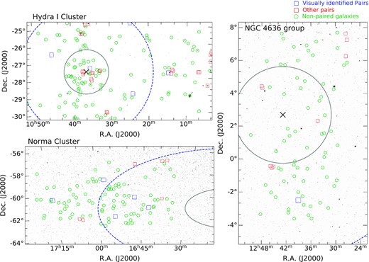
Integrated H i intensity map of the Hydra I cluster and WISE images of the Norma cluster, and the NGC 4636 fields. ASKAP H i detections from the SoFiA2 source finding are shown by the open red and blue rectangles (galaxy pairs) and green circles (non-paired control galaxies). The red rectangle hosts each member of a galaxy pair, and the larger blue one indicates a visually identified galaxy pair. The black cross symbols indicate the kinematic centres of the Hydra I and NGC 4636, and the references are given in Table 1. The grey solid and blue-dashed circles indicate the virial radius and a radius of three times the virial radius. See Section 2.1 for details.
The black cross mark, grey solid, and blue-dashed lines indicate the centres, virial radius, and a radius of three times the virial radius of the Hydra I and Norma clusters, and the NGC 4636 group. For the Norma field, only the eastern part is released due to strong continuum sources. The ASKAP pilot observations cover the Hydra I and Norma cluster fields out to approximately three times their virial radii within which the resolved H i gas distribution and kinematics of member galaxies can be studied. Kinematic properties and distances of the two galaxy clusters and the group are given in Table 1.
Properties of the Hydra I and Norma clusters and NGC 4636 group: (1) cluster or group name; (2) RA and Dec. of the centre position (J2000); (3) the distance to the cluster or group (Mpc); (4) the systemic velocity (|$\mathrm{km}\, \mathrm{s}^{-1}$|); (5) the velocity dispersion of the cluster or group (|$\mathrm{km}\, \mathrm{s}^{-1}$|); (6) the virial radius (Mpc); (7) the virial mass (1014M⊙); (8) references for columns (2–7): (a) Reynolds et al. (2021), (b) NED = NASA/IPAC Extragalactic Data base, (c) Woudt et al. (2008), (d) Jáchym et al. (2014), (e) Kilborn et al. (2009), (f) Osmond & Ponman (2004), and (g) Lee et al. (2022).
| Name | Centre | D | 〈V〉 | σ | Rvir | Mvir | Ref. |
|---|---|---|---|---|---|---|---|
| RA, Dec. (J2000) | (Mpc) | (|$\mathrm{km}\, \mathrm{s}^{-1}$|) | (|$\mathrm{km}\, \mathrm{s}^{-1}$|) | (Mpc) | (|$10^{14} \, \rm {M}_{\odot }$|) | ||
| (1) | (2) | (3) | (4) | (5) | (6) | (7) | (8) |
| Hydra I cluster | 10|$^{\rm {h}}36^{\rm {m}}41.\hskip-2.3pt^{\rm {s}}$|8, −27d31m28s | 61.0 | 3,777 | 676 ± 35 | 1.44 | 3.13 | a |
| Norma cluster | 16|$^{\rm {h}}15^{\rm {m}}32.\hskip-2.3pt^{\rm {s}}$|8, -60d54m30s | 69.6 | 4,871 | 925 | 2.20 | 11.0 | b, c, d |
| NGC 4636 group | 12|$^{\rm {h}}42^{\rm {m}}49.\hskip-2.3pt^{\rm {s}}$|8, + 02d41m16s | 13.6 | 1,696 | 284 ± 73 | 0.70 | 0.39 | b, e, f, g |
2.2 Galaxy classification: central, infalling, and outskirts galaxies
We classify member galaxies in Hydra I, Norma, and NGC 4636 based on their spatial and spectroscopic information. In the fields towards the clusters and galaxy group, there are background and foreground H i sources which are detected by SoFiA2. Given the systemic velocities of Hydra I (∼3777 |$\mathrm{km}\, \mathrm{s}^{-1}$|; Struble & Rood 1999), Norma (∼4,871 |$\mathrm{km}\, \mathrm{s}^{-1}$|; Woudt et al. 2008), and NGC 4636 (∼1,696 |$\mathrm{km}\, \mathrm{s}^{-1}$|; Kilborn et al. 2009), we only select H i sources whose systemic velocities are within the velocity ranges of 500–7000 |$\mathrm{km}\, \mathrm{s}^{-1}$|(cz < 7000 |$\mathrm{km}\, \mathrm{s}^{-1}$|), 500–9500 |$\mathrm{km}\, \mathrm{s}^{-1}$|(< 9500 |$\mathrm{km}\, \mathrm{s}^{-1}$|), and 500–3100 |$\mathrm{km}\, \mathrm{s}^{-1}$|(< 3100 |$\mathrm{km}\, \mathrm{s}^{-1}$|), respectively. These are five times the velocity dispersions of the clusters and the group with respect to their systemic velocities. This excludes the possibility of including any H i rich massive galaxies at high redshifts. The numbers of the identified galaxies according to the velocity cuts are 156, 109, and 83 in the Hydra I, Norma, and NGC 4636 fields, respectively.
Secondly, we classify the sample galaxies as three different groups: (1) central, (2) infalling, and (3) outskirts galaxies based on their locations in the phase-space diagrams of the galaxy clusters and group. For this, we use the projected phase-space diagrams of the Hydra I and Norma clusters and the NGC 4636 group. As shown in Fig. 2, the x-axis (r/Rvir) indicates the member galaxies’ projected distances from the centres that are normalized by their virial radii Rvir. The y-axis (ΔV/σdisp) indicates their relative line-of-sight velocities (ΔV) to the systemic velocities at the centres that are normalized by the velocity dispersions (σdisp) of the clusters and group. In many other works, this projected phase-space diagram has been widely used as a tool for classifying member galaxies as different groups with time since they infall into a galaxy cluster or group environment (Jaffé et al. 2015; Rhee et al. 2017; Yoon et al. 2017). Numerical simulations have shown that galaxies tend to follow a known path in the phase-space diagram as they fall into the cluster or group potential (Rhee et al. 2017).
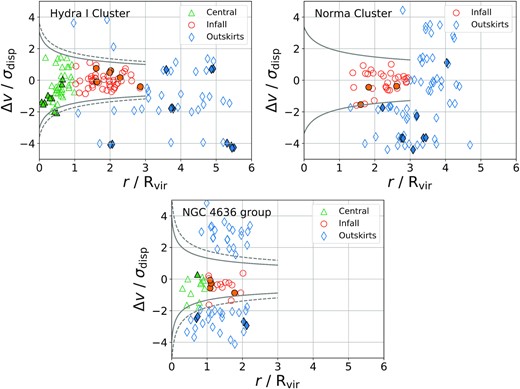
Phase-space diagrams of the Hydra I and Norma clusters, and NGC 4636 group. Galaxies are classified by their location on the phase-space diagram (see Section 2.2 for a description): central (green open triangles), infalling (orange open circles), and outskirts (blue open diamond) galaxies. Filled symbols indicate the corresponding galaxy pairs. The solid lines indicate the escape velocity curves of the clusters and the group which are derived using the equations (1–4) of Rhee et al. (2017). The dashed curves in the Hydra I cluster and the NGC 4636 group indicate the escape velocity curves to which 3 σesc and 1 σesc are added, respectively.
We define a galaxy as a central galaxy if its projected distance (r) from the cluster or group centre is < Rvir, and its line-of-sight systemic velocity with respect to the cluster or group systemic velocity divided by the cluster or group velocity dispersion, ΔV/σdisp, is less than an escape velocity limit of the cluster or group divided by the cluster or group velocity dispersion. The escape velocity (vesc) is derived using equations (1–4) of Rhee et al. (2017), which adopts the virial mass Mvir given in Table 1. We adopt (vesc ± 3σesc)/σdisp and (vesc ± 1σesc)/σdisp as the escape velocity limits for the Hydra I cluster and NGC 4636 group as in Reynolds et al. (2022) and Lee et al. (2022). These are shown as grey-dashed lines in Fig. 2. For the Norma cluster, we use vesc/σdisp as the limit since the cluster’s σesc is not available. If the projected distance (r) and normalized relative velocity (ΔV/σdisp) of a galaxy satisfy the following criteria, Rvir < r < 3Rvir and ΔV/σdisp < vesc/σdisp, we classify it as an infalling galaxy. Other galaxies with either ΔV/σdisp > vesc/σdisp or r > 3Rvir are classified as outskirts galaxies. The virial radii and masses of Hydra I and Norma clusters and the NGC 4636 group adopted in our work are derived assuming hydrostatic equilibrium (Hydra I), dynamical equilibrium (NGC 4636), or NFW halo (Norma). The values derived using the different assumptions are not very different within a range of up to a factor of 1.5. For more details, we refer to Reiprich & Böhringer (2002), Jáchym et al. (2014), and Lee et al. (2022) for Hydra I cluster, Norma cluster, and NGC 4636 group, respectively.
We show the locations of the central, infalling, and outskirts galaxies in the Hydra I, Norma, and NGC 4636 fields classified according to the above criteria on the phase-space diagrams in Fig. 2. They are colour-coded as green (triangle), orange (circle), and blue (diamond) colours, respectively in the figure. As discussed above, no central galaxies are classified in the Norma field due to the strong continuum sources in the cluster centre (see Fig. 1). The effect of continuum sources might have resulted in the asymmetric distribution of infall (orange) and central (green) galaxies relative to the systemic velocity for the Norma and NGC 4636 fields. Of the ASKAP H i detections in the three fields, we exclude galaxies whose H i emission is significantly affected by strong continuum sources or only partly detected. In our study, we focus on galaxy pairs at pre-merger stages, not the post-merger ones at coalescence. Hence, galaxies that appear to be in a post-merger stage are excluded. We identified post-merger galaxies both spatially and spectrally using their H i intensity and velocity maps, respectively. These are overlapped with each other in their H i intensity and velocity maps. On the other hand, the companions of a close galaxy pair are visually separated with each other in their H i intensity and velocity maps.
2.3 Sample selection of galaxy pairs and control galaxies
First, we compile galaxy pair candidates from the galaxies that are detected in H i and classified as the outskirts, infalling, or central ones in the three fields, the Hydra I, Norma, and NGC 4636 in Section 2.2. For this, we use the selection criteria described in Ventou et al. (2019), allowing us to select galaxy pair candidates based on their spectral and spatial information. Based on cosmological simulations, Ventou et al. (2019)’s selection criteria for closed pairs take into account 3D projection effects. If a system with two galaxies satisfies the following criteria, it is classified as a galaxy pair: the projected angular separation (Rp) and the absolute difference of the systemic velocities (ΔV) between the two galaxy encounters are within either (1) Rp ≤ 50 kpc and ΔV ≤ 300 |$\mathrm{km}\, \mathrm{s}^{-1}$| or (2) 50 kpc ≤ Rp ≤ 100 kpc and ΔV ≤ 100 |$\mathrm{km}\, \mathrm{s}^{-1}$|. This is compared with the ones typically adopted in other works, including Ellison et al. (2008) and Scudder et al. (2015), where a more relaxed criterion of ΔV ≤ 300–500 |$\mathrm{km}\, \mathrm{s}^{-1}$| is used. In addition, enhanced star formation rate (SFR) in galaxy pairs separated by Rp of ∼150 kpc has been found as in Patton et al. (2013). The galaxy pairs classified using our selection criteria are likely to be gravitationally bound. Together, their H i gas discs and systemic velocities should be resolved and separated by the ASKAP’s 30 arcsec beam (∼8.9, 9.8, and 2.0 kpc for the Hydra I, Norma clusters, and NGC 4636, respectively) and 4 |$\mathrm{km}\, \mathrm{s}^{-1}$| channel resolution, respectively. It is noted that we are targeting wet interactions as the galaxy pair candidates in this work are H i selected samples. There are 38 galaxy pair candidates selected by the selection criteria. Through a visual inspection of their H i data cubes, we find that most of them are well separated, either spectrally or spatially. These galaxy pair candidates can be in a stage of merging before the first encounter or after the first pericentre passage.
Additionally, we visually identify 10 galaxy pair candidates that are close to each other so that they are not separable in the H i emission detected by SoFiA2. These close galaxy pair candidates could be in a late stage of merging where the two interacting galaxies are not coalescent yet but overlapped spatially and/or spectrally. This could make their systemic velocities comparable with each other. These galaxy pair candidates are visually verified and indicated by the symbol, ‘*’ in Tables A2 and A7. An example of a visually identified close galaxy pair candidate, which can be in a late stage of the galaxy merger sequence, is presented in Fig. 3. Of all the galaxies detected at H i in the three fields, there are 48 galaxy pair candidates selected by either the above selection criteria (38 galaxies) or our visual inspection (10 galaxies; see FigsA1–A3 in Appendix; the full tables and figures are available as supplementary online material). These are subsequently classified as the outskirts, infalling, and central galaxy pairs based on their locations in the phase-space diagrams of Fig. 2.
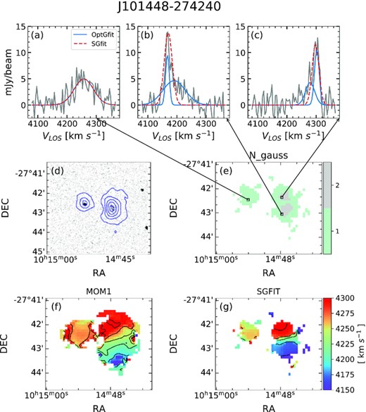
Velocity profiles and H i maps of a galaxy pair J101448 − 274240 in the Hydra I cluster. (a–c): the blue-solid and red-dashed lines indicate the optimal Gaussian fitting (OptGfit) and single Gaussian fitting (SGfit) to the observed profiles (grey solid lines) at three locations. (d): WISE images overlaid with the contours of the H i integrated intensity (moment0) maps; the contours start from 0.075 Jy beam−1 in steps of 0.125 Jy beam−1, (e): 2D map of the optimal number of Gaussian components, (f): moment1 map (MOM1), and (g): single Gaussian fitting velocity field (SGFIT).
H i gas mass-ratio values for the galaxy pairs range from 1:1.6 to 1:66.6 with the peak value being between 1:1 and 1:6. Simulations predict that minor mergers with dynamical mass ratios 1:10 or less do not usually produce significant morphological disturbance in their gas and stellar distributions (e.g. Hernández-Toledo et al. 2005; Conselice 2006). In general, such morphological disturbances are more enhanced in major mergers with mass ratios of 1:4 or closer to unity. In this respect, our fnarrow and Toomre-Q parameter measurements might better extract any kinematic disturbances (if present) even in minor mergers even though the H i mass ratio may not directly scale with the dynamical or stellar mass ratio.
Secondly, as a control sample, we select a set of galaxies in the Hydra I, Norma, and NGC 4636 fields, which do not satisfy the selection criteria above and thus have no close companions in their spatial and spectral vicinity. These control galaxies are relatively less affected by the gravitational effects of any close companions compared to the galaxy pair candidates selected above. From these, 266 control sample galaxies are selected in the three fields. Likewise, these are classified as the outskirts, infalling, and central galaxies according to their locations in the phase-space diagrams. H i properties of these control galaxies will be compared with those of the galaxy pairs.
We make additional cuts to both the galaxy pairs and the control sample galaxies above in order to match the distribution of their H i masses and the galaxy number ratios (outskirts/infalling and outskirts/central) between the different environments in the three fields. This is to reduce potential bias due to differences in the galaxy number ratios for the clusters and group or in galaxy properties. Since we examine how the small-scale kinematics and kinematically cool-to-total H i mass ratio of galaxies are affected in galaxy pairs and cluster environments at fixed total H i mass, we match the sample galaxies by H i mass. Here, we assume that the sample galaxies on average have not yet been significantly affected by the cluster environment.
The H i mass and galaxy number ratio cuts are made based on the galaxies in the Hydra I field as both the Norma and NGC 4636 fields are affected by continuum sources as discussed in Section 2.1. When matching the H i mass distribution and galaxy number ratios for the galaxy pairs and control galaxies selected above, we preferentially remove the ones which are relatively less resolved by the ASKAP beam and with low signal-to-noise (S/N). We exclude sources which are less resolved (across their major axes) than two, four, and five synthesized beams in the Hydra, Norma, and NGC 4636 fields, respectively. The corresponding S/N of individual H i profiles of the selected galaxies is greater than three. The resulting H i mass distribution for the final sample galaxies is shown in Fig. 4. The H i mass distribution of the infalling galaxy pairs is narrower than that of the control galaxies due to the lack of galaxy pairs in the H i mass bins (< 8.45). The corresponding galaxy number ratios (Outskirts/Infall and Outskirts/Central) for the galaxy pairs and control galaxies in the Hydra I, Norma, and NGC 4636 fields are given in Table 2.
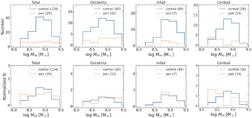
The H i mass distribution of the galaxy pairs and control sample galaxies of the Hydra I, Norma clusters, and NGC 4636 group in the outskirts, infalling, and central environments as denoted on the top of each panel. The mass distribution of all the sample galaxies are shown in the left-most panels. The orange-dashed and blue-solid lines show the galaxy pairs and control sample galaxies, respectively. The number of the control galaxies and galaxy pairs are denoted.
The number of galaxy pairs (indicated by ‘*’ symbol) and control sample galaxies, and the galaxy number ratios, N(outskirts)/N(infall) and N(outskirts)/N(central) in the Hydra I, Norma, and NGC 4636 fields.
| N(Outskirts) | N(Infall) | N(Central) | N(Outskirts)/N(Infall) | N(Outskirts)/N(Central) | |
|---|---|---|---|---|---|
| Hydra I | 24 | 30 | 30 | 0.80 | 0.80 |
| 9* | 5* | 10* | 1.80* | 0.90* | |
| Norma | 13 | 12 | – | 1.08 | – |
| 1* | 1* | –* | 1.0* | –* | |
| NGC 4636 | 5 | 4 | 6 | 1.25 | 0.83 |
| 2* | 1* | –* | 2.0* | –* |
In summary, 29 galaxy pair candidates (Hydra I: 24, Norma: 2, and NGC 4636: 3) and 124 control sample galaxies (Hydra I: 84, Norma: 25, and NGC 4636: 15) are selected by the selection criteria adopted in this work. The H i images (moment maps, single Gaussian fitting, and model velocity fields) of the galaxy pairs are shown in Figs A1–A3 in Appendix (the full figures are available as supplementary online material). The observational properties of the sample galaxies, including their H i properties derived in this work, are presented in TablesA1–A6 in Appendix (the full tables are available as supplementary online material).
3 H i data analysis
3.1 Decomposition of H i velocity profiles
We perform profile decompositions of individual line-of-sight line profiles of the ASKAP H i data cubes. For this, we use a newly developed profile decomposition tool, baygaud (Oh et al. 2019a). For each line profile of an H i data cube, baygaud performs profile decomposition based on Bayesian nested sampling techniques, and finds an optimal number of Gaussian components with which the profile is best described.
From the performance test discussed in Oh et al. (2019a), baygaud is found to be robust for parameter estimation and model selection against any local minima in the course of the fitting as long as the integrated S/N of the line profile is high enough for the analysis, for example, larger than three or so. We refer to Oh et al. (2019a) for the full description of the fitting algorithm and its performance test (see also Oh et al. 2022 and Park et al. 2022).
We run baygaud for the ASKAP H i data cubes, letting it fit the individual velocity profiles with the models in equation (1) consisting of different numbers of Gaussian components starting from one up to a user-defined maxim number. From a visual inspection of line profiles of the cubes, we find that modelling them with up to three Gaussian components appears to be enough to take their non-Gaussian profile shape into account. In this work, we adopt the maximum number of Gaussian components as three for the baygaud analysis. In addition, baygaud is only ran over the line profiles of the cubelets within the SoFiA2 masks whose S/N is greater than three. As described in Oh et al. (2019a), we select the most appropriate model for each H i velocity profile among the competing Gaussian models with one, two, and three Gaussian components based on their calculated Bayesian evidence. In this work, we adopt the ‘substantial’ model whose Bayes factor against the second-best model is at least larger than 3.2. In the rest of this paper, we designate the best model as ‘optimal Gaussian fitting’. If the data are best described by a single Gaussian component, we call it ‘single Gaussian fitting’.
In Fig. 3, examples of line profiles are given by the grey solid lines, and the blue-solid and red-dashed lines represent their optimal Gaussian fitting and single Gaussian fitting results, respectively. The single Gaussian fitting loses part of the flux, which is unsuitable for accounting for the non-Gaussianity of the profiles. On the other hand, the optimal Gaussian fitting better models the non-Gaussian profiles, retrieving more flux than the single Gaussian fitting. For example, the total integrated intensity of J101448 − 274240 derived from the single Gaussian fitting analysis is 63.3 Jy beam−1, which is approximately 7|${{\ \rm per\ cent}}$| lower than that derived from the optimal Gaussian fitting analysis with 68.0 Jy beam−1. The number of optimally decomposed Gaussian components is mapped in the panel (e) of Fig. 3. This map visualizes the non-Gaussian feature of the line profiles in a quantitative manner.
3.2 H i rotation curves
We derive the H i rotation curves of the sample galaxies whose number of resolved elements across the major axis by the ASKAP’s 30 arcsec beam is at least larger than five (≥6) on their single Gaussian fitting velocity fields. There are 77 galaxies available for the H i rotation curve analysis. As described in Section 3.1, we mask the pixels of the velocity fields that do not satisfy the integrated S/N limit of three for their line profiles. An example single Gaussian fitting velocity field of a galaxy pair classified, as in Section 2.3, is presented in panel (g) of Fig. 3. We note that these single Gaussian fitting velocity fields, which are based on the line profile fitting analysis, are less affected by any spike-like noise in the line profiles, and thus better estimate their representative centroid velocities than the conventional moment analysis (moment1) in most cases.
However, the single Gaussian fitting method has limited success in modelling non-Gaussian profile shapes (e.g. Oh et al. 2022). Alternative fitting forms, on the other hand, such as the Hermite polynomial and multiple Gaussian functions, have worked in other cases (de Blok et al. 2008; Oh et al. 2008, 2011, 2015, 2022). Since the main purpose of the rotation curve analysis in this work is to derive rotation velocities at a given radius in order to calculate the gravitational instabilities of the gas disc, and their geometrical parameters which are used to measure H i morphology, the use of single Gaussian fitting velocity fields is adequate. However, there are two galaxies whose single Gaussian fitting velocity field maps have large blank areas due to low S/N. For these galaxies, we instead use their SoFiA2 moment1 maps for the rotation curve anlaysis. These galaxies are indicated by ‘*’ symbol in Table A1– A6.
To derive the rotation curves of the sample galaxies, we use 2D Bayesian Automated Tilted-ring fitter (2dbat; Oh et al. 2018), which allows us to fit 2D tilted-ring models to a velocity field in a fully automated manner based on Bayesian analysis techniques. We refer to Oh et al. (2018) for the full description of 2dbat, which describes its detailed fitting algorithm and performance test using simulated and observed H i data cubes.
In the course of the non-parametric 2D tilted-ring analysis which fits concentric tilted-rings to the observed velocity field, the kinematic centre (XPOS, YPOS) and systemic velocity (VSYS) of a galaxy can be modelled with single values over all the rings. On the other hand, we adopt a cubic spline curve to model the rotation velocity parameter (vROT), which varies with galaxy radius in the analysis.
Given the regularization setup of the ring parameters, we derive two rotation curves (ϕ: cubic spline, i: constant) for each galaxy. The 2dbat analysis was performed on all the galaxy pairs (48) and control galaxies (266) which are not matched in H i mass and galaxy number ratios, and performed adequately in 77 cases (∼25 per cent). The exceptions, 237 cases, are significantly disturbed by non-circular motion or not well resolved and hence were excluded from further rotation curve analysis. Most galaxies show no significant radial variations of ϕ and i in the cubic-spline fits, providing comparable best-fitting measurements of ϕ and i between the two regularization setup (i.e. constant and cubic spline) within their uncertainties. No evidence of overfitting of ϕ and i using the cubic splines is seen in the analysis from visual inspection. In Fig. 5, we show the distributions of i, ϕ, and VSYS of the 77 sample galaxies, derived from the tilted-ring analysis.
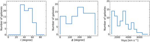
Distributions of inclination (i), position angle (ϕ), and systemic velocities (VSYS) values of 77 sample galaxies from the rotation curve analysis.
3.3 H i superprofiles of the sample galaxies
For each galaxy in our sample, we stack individual line profiles of the data cube after aligning their centroid velocities to derive the so-called ‘H i superprofile’ as described in Ianjamasimanana et al. (2012). In general, the S/N of the superprofile stacked using independent profiles increases with |$\sqrt{N}$|, where N is the total number of the co-added profiles since the noise decreases as |$1/\sqrt{N}$|. Several studies have used superprofiles of galaxies, constructed using H i or CO data cubes, in order to investigate correlations between the superprofile velocity dispersion and physical properties of galaxies (e.g. metallicity, far-UV (FUV)-near-UV (NUV) colours, and H α luminosities; see Ianjamasimanana et al. 2012; Stilp et al. 2013; Hunter et al. 2022). In addition, a superprofile can be decomposed into double Gaussian components, which can be then classified as kinematically narrow and broad Gaussian components representing narrower and broader velocity dispersions, respectively. Based on the analysis of THINGS6 galaxies, Ianjamasimanana et al. (2012) show that the narrower (kinematically cool) H i component of the superprofiles are likely to be associated with SF and possibly with molecular hydrogen gas.
In this work, we construct superprofiles of the sample galaxies using their decomposed H i gas components from baygaud analysis in Section 3.1. The superprofile stacking analysis that we adopt is as follows:
Decompose individual H i line profiles into optimal numbers of Gaussian components using baygaud; determine their central velocities from the Gaussian fitting.
For the extraction of each Gaussian component of a line profile, we subtract the other Gaussian model components from the original line profile. If the profile is best described by a single Gaussian function, use the input velocity profile whose central velocity is determined from the single Gaussian fitting.
Align all the residual line profiles from which the other Gaussian models are subtracted with respect to their centroid velocities; use the original line profiles for the alignment if they are best modelled by a single Gaussian function.
Construct the H i superprofile by co-adding all the aligned line profiles.
Fit a double Gaussian model to the superprofile; use the velocity channels whose velocities are within ± three times velocity dispersion with respect to the central velocity of the superprofile; the velocity dispersion and the central velocity are derived by fitting a single Gaussian function to the superprofile; this prevents us fitting unreasonably broad velocity dispersions, which might be caused by background ripples that result from inaccurate baseline subtraction.
Derive the amplitudes, velocity dispersions, and central velocity of the primary and secondary Gaussian components and constant background as a means to quantify the superprofile.
The Gaussian model parameters are estimated using the python module emcee with a prior range of δV < velocity dispersion (σ) < 150 |$\mathrm{km}\, \mathrm{s}^{-1}$|, and −3 × δV < central velocity < +3 × δV, where δV is the channel resolution. In this work, we do not include line profiles whose integrated S/N is less than three when constructing the superprofiles. We note that the optimally decomposed line profiles whose central velocities are determined from the Gaussian fitting are stacked to produce the superprofiles. This is compared with the previous stacking methods that align the line profiles to their central velocities determined from the moment analysis (intensity-weighted mean velocity) or Hermite polynomial fit.
In Fig. 6, we show the ranges of full width at half-maximum (FWHM) values of the narrow and broad components in the H i superprofile analysis. The blue-dashed and orange-solid lines indicate the FWHM values of narrow and broad components, respectively. Approximately, they range from 10 |$\mathrm{km}\, \mathrm{s}^{-1}$|to 119 |$\mathrm{km}\, \mathrm{s}^{-1}$|and 20 |$\mathrm{km}\, \mathrm{s}^{-1}$|to 226 |$\mathrm{km}\, \mathrm{s}^{-1}$|, respectively. The mode values of the distributions for the narrow and broad components indicated by the solid vertical lines are ∼25 and ∼85 |$\mathrm{km}\, \mathrm{s}^{-1}$|, respectively. For this, we also derive additional H i superprofiles of a sample galaxy, J101247 − 275028, using the centroid velocities of line profiles determined from the moment analysis (moment0) and the Hermite h3 polynomial fitting. We then compare them with the baygaud-based H i superprofile as shown in Fig. 7. Turbulent gas motions caused by hydrodynamical processes in galaxies like SF or supernova (SN) explosions can result in larger velocity dispersions and asymmetric tails to H i velocity profiles. A superprofile constructed using these asymmetric non-Gaussian line profiles with larger velocity dispersions will have broader wings and lower peaks than the one constructed using the decomposed Gaussian profiles which tend to have smaller velocity dispersions. We refer to Kim & Oh (2022) for the full description of the superprofile stacking analysis adopted in this work and its comparison with the previous methods using THINGS and LITTLE THINGS7 sample galaxies.
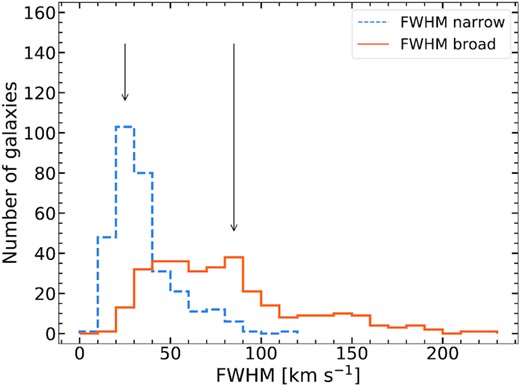
Distributions of FWHM values of narrow and broad components for all sample galaxies. The blue-dashed and orange-solid lines indicate the FWHM values of the narrow and broad components, respectively. The arrows indicate the mode value of each component.
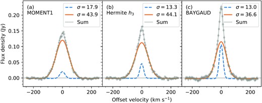
H i superprofiles of J101247-275028 derived from the three profile analysis methods: (a) moment analysis; (b) Gauss-Hermite h3 polynomial fitting; and (c) baygaud analysis with double Gaussian fitting. Grey dots show the corresponding H i superprofiles, and the blue-dashed and orange-solid lines indicate the narrow and broad components decomposed from the double Gaussian fitting. The grey solid lines are the sum of the narrow and broad components. The derived velocity dispersions of the narrow and broad components are denoted on the top-right corner of the panels.
The influence of galaxy–galaxy interactions, or merging processes, on the gas distribution and kinematics of galaxies that experience close encounters varies for in different parts of a galaxy; i.e. core and outer regions (Olson & Kwan 1990; Barnes & Hernquist 1991; Yamashita et al. 2017; Moreno et al. 2021). Accordingly, this can lead to different spatial distribution and SF rates on a range of time-scales in the galaxies (Saintonge et al. 2012; Wang et al. 2022). Many post-merger galaxies show enhanced SF in their central kpc region (Ellison et al. 2013). This is mainly attributed to the inflow of interstellar medium into the central regions of the galaxies, which results in the formerly atomic medium being compressed and thus converted into molecular gas due to the higher hydrostatic pressures (Moreno et al. 2021).
In this regard, we also split the inner and outer gas disc regions of the sample galaxies at an H i break radius, |$R_{\rm {H\, \small {\rm I}-break}}$|. For each sample galaxy, we derive two additional superprofiles for the central and outer regions, as well as the one for the entire gas disc region. As a |$R_{\rm {H\, \small {\rm I}-break}}$|, we adopt 0.5|$R_{\rm {H\, \small {\rm I}}}$| based on which the H i properties of the superprofiles for the central and outer regions show the most significant change with respect to the galaxy environments. |$R_{\rm {H\, \small {\rm I}}}$| is the radius of H i disc defined at a surface density (|$\sum _{\rm {H\, \small {\rm I}}}$|) of 1 |$\rm {M_{\odot } \, pc^{-2}}$| in the |$\sum _{\rm {H\, \small {\rm I}}}$| radial profile. To derive |$R_{\rm {H\, \small {\rm I}}}$|, we use the H i mass–size relation (Broeils & Rhee 1997; Wang et al. 2016). These regional superprofiles will be useful for examining how the H i gas properties react with the gravitational impact of galaxies in different galaxy environments.
The H i superprofiles of galaxy pair candidates in the Hydra I, Norma clusters, and NGC 4636 group are presented in Figs A4–A6 in Appendix (the full superprofile figures are available as supplementary online material). We classify the decomposed Gaussian profiles of an H i superprofile as kinematically narrow and broad components with respect to their velocity dispersions (σ). Relatively, the kinematically narrow component has a smaller σ than the broad one.
3.4 Toomre Q parameter
Gas instability leads to gravitational collapse, and SF is expected in regions where the observed gas surface density Σgas is higher than the critical surface density Σcrit, that is, Σgas/Σcrit > 1, which means Qgas < 1. Below this so-called SF threshold, gas pressure stabilizes the gas cloud against gravitational collapse. This Toomre Q criterion is analogous to the Jeans criterion, but it includes the kinematic effect of the disc’s rotation.
In equation (7), we use the gas surface density summed over the optimally decomposed Gaussian components. We then multiply by a factor of 1.4 to the H i gas surface density derived in order to take the amount of helium and metal abundances of the gas into account. To estimate κ in equation (8), we adopt the rotation curves derived from the 2dbat analysis in Section 3.2. As κ is derived from the rotation curve analysis, we only select galaxies which show a clear rotation pattern in their H i velocity fields and that have intermediate values of inclination (30° < i < 70°), and are resolved with ≥ 6 beams across their major axes.
For the gas velocity dispersion in equation (7), we use the velocity dispersion values derived from the single Gaussian fitting to the H i velocity profiles. As for the H i superprofiles derived in Section 3.3 for each galaxy, we derive Toomre Q parameters over the central (|$0 \lt r \lt 0.5R_{\rm {H\, \small {\rm I}}}$|), outer (|$0.5R_{\rm {H\, \small {\rm I}}}$||$\lt r \lt R_{\rm {H\, \small {\rm I}}}$|), and entire (|$0 \lt r \lt R_{\rm {H\, \small {\rm I}}}$|) disc regions.
In theory, if Qgas < 1, the disc is expected to become gravitationally unstable and trigger SF. However, Leroy et al. (2008) and Romeo & Mogotsi (2017) found that star-forming galaxies often have Qgas values above unity. This is because the Toomre Q criterion assumes a simple disc model of symmetric perturbations and we assume a pure gas disc. Therefore, we should keep in mind that the Toomre Q analysis is limited in identifying the local disc gravitational instability in a disturbed gas disc.
In Fig. 8, we present an example 2D map of the Toomre Q values of a galaxy, J123228 + 002315, overlaid with the orange contours of Qgas < 2, which indicate gravitationally unstable regions (Zheng et al. 2013, Wong et al. 2016). From this, we are able to identify gravitationally unstable candidate regions where Qgas < 2 corresponding to Σgas/Σcrit > 2. As shown in Fig. 8, the Qgas values in the central and outer regions are higher. However, this might be due to an overestimated gas velocity dispersion of H i velocity profiles that are presumably caused by the effect of the beam resolution (so-called beam smearing). Given this, the estimated Qgas values can be considered as upper limits for the gravitational instability of the gas disc.
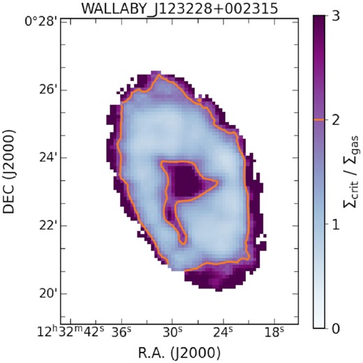
A 2D map of the Toomre Q parameter values as indicated in the colourbar for J123228 + 002315. The regions with Qgas < 2 are enclosed by the orange contours.
3.5 H i asymmetry
The morphological asymmetry of the moment0 can be measured by summing the absolute residuals between the two maps, I and I180. We rotate the SoFiA2 moment0 map of a galaxy with respect to its kinematic centre derived from the 2bdat analysis. We refer to Reynolds et al. (2020) for the full description of measuring the H i morphological asymmetry of a galaxy. As an example, Fig. 9 shows the H i intensity maps (the original, 180° rotated, and residual ones) of a galaxy, J104016 − 274630. The |$A_{\rm {map}}^{\rm {H\, \small {\rm I}}}$| value for this galaxy derived using equation (10) is 0.19. The larger the value of |$A_{\rm {map}}^{\rm {H\, \small {\rm I}}}$|, the more asymmetric H i gas distribution is.
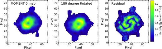
The H i integrated-intensity maps of J104016 − 274630 used for deriving the galaxy’s morphological H i asymmetry. Left: H i moment0 map, middle: H i moment0 map rotated 180°, and right: the absolute residual map as indicated in the colourbar. See Section 3.5 for more details.
Both internal and external hydrodynamical effects of galaxies, such as gas outflows driven by SF or SN explosions, ram pressure stripping, and tidal interactions between galaxies, can make the gas disc of galaxies disturbed, particularly in the outer regions (Gunn & Gott 1972; Barnes & Hernquist 1996; Martin 2005). The analysis of the morphological H i asymmetry in different environments is useful for investigating how environments affect the H i distribution of galaxies. This is discussed in Section 4.
4 ENVIRONMENTAL EFFECTS ON THE RESOLVED H i PROPERTIES OF GALAXY PAIRS
In this section, we examine the effects of galaxy environment (outskirts, infalling, and central) on the resolved H i properties of galaxy pairs in the two clusters (Hydra I and Norma) and the galaxy group (NGC 4636). The following analyses are carried out: (1) First, we investigate how the fractions of the kinematically decomposed narrow H i gas components in the total H i gas of galaxy pairs and control sample galaxies change with the infall stage (i.e. central, infalling, and outskirts). (2) Secondly, we assess whether the infall stage has an impact on the gravitational instability of gas discs using the Toomre Q parameters. (3) Thirdly, we inspect the morphological H i asymmetries of galaxies to see whether there is any systematic difference between the pairs and control galaxies in the environments. Using these analyses, we examine whether the resolved H i properties of the sample galaxies are affected by the galaxy environments in a quantitative manner.
4.1 Kinematically narrow H i gas
It has been shown that galaxy mergers and strong tidal interactions of gas-rich galaxies can trigger SF (Mihos & Hernquist 1996; Di Matteo et al. 2007; Ellison et al. 2013; Patton et al. 2013). On the other hand, galaxy cluster and group environments are more likely to quench SF as galaxies reach close to the cluster or group centre (Cortese et al. 2011; Boselli et al. 2016; Cortese et al. 2021).
Molecular hydrogen in galaxies serves as a gas reservoir for SF, which is sustained and/or fed from cool H i gas (e.g. Bigiel et al. 2008; Saintonge & Catinella 2022). In the course of forming the molecular hydrogen gas, atomic hydrogen should have passed the kinematically narrow (cool) H i gas before turning into H2. Thus, the kinematically narrow H i gas components decomposed from the stacked profiles in Section 3.3 may be associated with the H2 component (e.g. Ianjamasimanana et al. 2012).
Here, we investigate the influence of galaxy environments associated with the infall stage on the kinematically narrow H i gas components of the sample galaxies. Fig. 10 shows the mass fractions of the kinematically narrow H i gas in the total H i masses, fnarrow = |$M_{\rm {narrow}}^{\rm {H\, \small {\rm I}}}$| / |$M_{\rm {total}}^{\rm {H\, \small {\rm I}}}$|, derived for the three different disc regions of the sample galaxies. In addition, these are shown for the different galaxy environments, outskirts, infalling, and central as classified in Section 2.2. Here, we use all the sample galaxies in the three fields, the Hydra I, Norma clusters, and NGC 4636. The mass fractions for the galaxy pairs and control galaxies are displayed with different colours, galaxy pair (orange) and control galaxy (blue). The numbers of the control and pair (bracket) galaxies in the galaxy environment bins are denoted on each panel in Fig. 10.
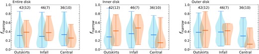
Distributions of the kinematically narrow H i gas fractions fnarrow = |$M_{\rm {narrow}}^{\rm {H\, \small {\rm I}}}$| / |$M_{\rm {total}}^{\rm {H\, \small {\rm I}}}$| of the three different regions (‘Entire’, ‘Inner’, and ‘Outer’) of the sample galaxies in the outskirts, infalling, and central environments. The control galaxies and galaxy pairs are shown with blue and orange colours, respectively. The numbers of the control and pair (bracket) galaxies are shown in each panel. The border thickness represents the relative frequency of the sample galaxies with the corresponding fnarrow values. The small horizontal lines in each panel indicate the median values.
As shown in Fig. 10, the median fnarrow values indicated by the thick horizontal lines for the entire disc do not appear to vary much over the environments for the control galaxies (blue). The median fnarrow values of the infalling galaxies are slightly higher in both the inner and outer disc regions than the others in the outskirts and central environment. Despite the wide range of the fnarrow values for the outer disc region of the control galaxies, the median value is the lowest in the central environment although it is not significant. More frequent galaxy interactions are expected in the central environment with higher local densities, which could give rise to more turbulent gas motions with higher velocity dispersions.
The ram pressure caused by the intergalactic medium (IGM) could also have influenced the fnarrow values of galaxies in the central environment. It could strip part of the kinematically narrow H i gas in denser environments (Chung et al. 2009; Cortese et al. 2011; Catinella et al. 2013; Jaffé et al. 2016; Brown et al. 2017; Wang et al. 2021). Molecular hydrogen (H2) gas in galaxies traced by CO emission, particularly in the outer regions, can also be stripped by ram pressure in a cluster environment (Boselli et al. 2014; Chung et al. 2017; Castignani et al. 2018; Cortese et al. 2021; Stevens et al. 2021).
The removal of cool H i gas by ram pressure stripping will in turn lead to SF quenching (Koopmann & Kenney 2004; Boselli & Gavazzi 2006; Jaffé et al. 2015). Additionally, numerous high-speed galaxy encounters, i.e. ‘galaxy harassment’ can increase the gas velocity dispersion of galaxies in the denser environment (Moore et al. 1996). This in turn will decrease their fnarrow values. In the course of galaxy harassment, the cool (kinematically narrow) H i component can be heated, which results in a higher velocity dispersion.
As shown in Fig. 10, the median fnarrow values for the three disc regions (entire, inner and outer) of galaxy pairs (orange) are the lowest in the central environment. The gravitational effect of the close galaxy pairs may play a role in inducing the trend. As discussed in Ellison et al. (2010), SF triggered by galaxy–galaxy interaction is more enhanced in the outskirts (i.e. field) than in dense environments. This is likely to be associated with the higher fnarrow values of galaxy pairs in low-density environments as found in this work (see also Vollmer et al. 2012; Stierwalt et al. 2015; Lee et al. 2017). Marasco et al. (2016) concluded that the satellite encounters are more effective at stripping H i gas than ram pressure stripping in the dense environment using the EAGLE simulations. We note that the difference in H i mass distribution between the environments (outskirts, infalling, and central) may impact the fnarrow trend found in this work. As shown in Fig. 4, the fraction of galaxies in low |$M_{\rm {H\, \small {\rm I}}}$| mass bins (|${\rm log\, M_{H\, \small {\rm I}}}$| < 8.7) is relatively lower in the infalling and central regions than in the outskirts. In these denser infalling and central environments, galaxies may have already experienced moderate gas loss which is below the current WALLABY’s sensitivity. However, it is difficult to predict how exactly this process affects the fnarrow trend in the subcluster environments due to the low number statistics. A larger sample of galaxies is needed to further improve the analysis. In addition, we also note that there are a number of sample galaxies (∼11 and 7|${{\ \rm per\ cent}}$| of the control and paired galaxies) that have similar velocity widths (velocity dispersion difference < ASKAP channel resolution of 4 |$\mathrm{km}\, \mathrm{s}^{-1}$|) of the narrow and broad components in the H i superprofile analysis. These galaxies are denoted with a † symbol in Table A1–A6. This could be attributed to factors like low S/N, fractions of cool or warm gas components over the total gas, etc. A scaled single Gaussian model fit would be appropriate for measuring global velocity dispersions of these superprofiles, as described in Stilp et al. (2013). In this work, since we need to decompose the superprofiles into kinematically narrow and broad components, a double Gaussian model fit is made to the profiles. We tabulate the median and standard deviations of the fnarrow values derived for the entire, inner, and outer gas discs of the sample galaxies in Table 3.
The median values (〈fnarrow〉median) and standard deviations (|$\sigma _{f_{\rm {narrow}}}$|) of the kinematically narrow H i gas fractions for the three disc regions (entire, inner, and outer) of the galaxy pai and control sample galaxies in the outskirts, infalling, and central environments. N is the number of samples, and CI denotes the 95 |${{\ \rm per\ cent}}$| confidence interval for median value.
| Outskirts | Infalling | Central | |||||||||||
|---|---|---|---|---|---|---|---|---|---|---|---|---|---|
| 〈fnarrow〉median | 1σ | CI | N | 〈fnarrow〉median | 1σ | CI | N | 〈fnarrow〉median | 1σ | CI | N | ||
| Entire | Control | 0.31 | 0.21 | (0.22, 0.39) | 42 | 0.29 | 0.22 | (0.21, 0.46) | 46 | 0.33 | 0.21 | (0.26, 0.45) | 36 |
| Pair | 0.39 | 0.18 | (0.27, 0.54) | 12 | 0.38 | 0.17 | – | 7 | 0.26 | 0.16 | (0.09, 0.56) | 10 | |
| Inner | Control | 0.28 | 0.20 | (0.20, 0.45) | 42 | 0.35 | 0.19 | (0.25, 0.42) | 46 | 0.33 | 0.19 | (0.21, 0.40) | 36 |
| Pair | 0.42 | 0.22 | (0.20, 0.69) | 12 | 0.48 | 0.21 | – | 7 | 0.15 | 0.23 | (0.08, 0.71) | 10 | |
| Outer | Control | 0.38 | 0.22 | (0.25, 0.47) | 42 | 0.39 | 0.20 | (0.30, 0.49) | 46 | 0.30 | 0.20 | (0.24, 0.47) | 36 |
| Pair | 0.43 | 0.23 | (0.23, 0.68) | 12 | 0.42 | 0.18 | – | 7 | 0.12 | 0.17 | (0.05, 0.49) | 10 | |
The median values (|$\langle \rm {Q} \rangle ^{\rm {median}}$|) and standard deviations (σQ) of the Toomre Q parameter values for the three disc regions (entire, inner, and outer) of the galaxy pairs and control sample galaxies which are not matched (upper) and matched (lower) in H i mass and galaxy number ratios, respectively, in the outskirts, infalling, and central environments. N is the number of samples, and CI denotes the 95|${{\ \rm per\ cent}}$| confidence interval for median value.
| Outskirts | Infalling | Central | |||||||||||
|---|---|---|---|---|---|---|---|---|---|---|---|---|---|
| |$\langle \rm {Q} \rangle ^{\rm {median}}$| | 1σ | CI | N | |$\langle \rm {Q} \rangle ^{\rm {median}}$| | 1σ | CI | N | |$\langle \rm {Q} \rangle ^{\rm {median}}$| | 1σ | CI | N | ||
| Entire | Control | 3.08 | 8.87 | (2.24, 6.30) | 37 | 6.28 | 7.87 | (3.14, 11.9) | 18 | 7.01 | 8.56 | (3.70, 32.68) | 10 |
| Pair | 2.58 | 1.24 | – | 8 | 6.50 | 3.01 | – | 2 | 31.36 | 19.55 | – | 2 | |
| Inner | Control | 3.96 | 12.56 | (2.74, 6.05) | 37 | 7.77 | 12.12 | (3.56, 11.05) | 18 | 8.10 | 21.54 | (3.82, 78.2) | 10 |
| Pair | 1.57 | 1.04 | – | 8 | 4.06 | 0.60 | – | 2 | 36.98 | 18.07 | – | 2 | |
| Outer | Control | 3.45 | 8.20 | (2.53, 6.32) | 37 | 5.23 | 5.26 | (3.27, 8.12) | 18 | 6.32 | 7.65 | (3.15, 29.14) | 10 |
| Pair | 2.54 | 1.98 | – | 8 | 7.56 | 4.00 | – | 2 | 26.99 | 16.14 | – | 2 | |
| Entire | Control | 3.08 | 4.77 | (2.20, 11.8) | 11 | 9.02 | 5.01 | – | 4 | 5.95 | 10.65 | – | 6 |
| Pair | 0.96 | 0.91 | – | 4 | 3.50 | 0.00 | – | 1 | 31.36 | 19.55 | – | 2 | |
| Inner | Control | 2.74 | 5.31 | (1.80, 9.86) | 11 | 9.04 | 6.23 | – | 4 | 8.72 | 26.80 | – | 6 |
| Pair | 1.10 | 0.49 | – | 4 | 3.46 | 0.00 | – | 1 | 36.98 | 18.07 | – | 2 | |
| Outer | Control | 3.45 | 6.94 | (2.58, 13.47) | 11 | 5.39 | 5.88 | – | 4 | 4.88 | 9.54 | – | 6 |
| Pair | 0.89 | 1.81 | – | 4 | 3.55 | 0.00 | – | 1 | 26.99 | 16.14 | – | 2 | |
Ellison et al. (2018) argue that merger-induced SF quenching is not via exhaustion or expulsion of the gas reservoir. Instead, it could be due to enhanced turbulent gas motions, which make the gas reservoir less capable of forming stars. The decreasing trend of the median fnarrow values for the galaxy pairs in the central environment seen in our work seems to support such a scenario. In Fig. 11, we show the fnarrow values for the three disc regions (entire, inner, and outer) of galaxy pairs with their H i masses, and compare them with those of non-paired galaxies in the outskirts, infall, and central environments. For this, we use 48 galaxy pairs and 266 non-paired galaxies detected at H i in the Hydra I, Norma, and NGC 4636 fields from the ASKAP pilot observations.
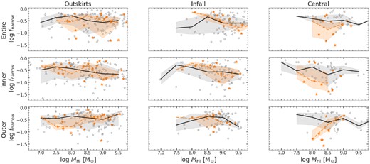
The kinematically narrow H i gas fractions for the three disc regions (entire, inner, and outer) of sample galaxies with their H i masses in the outskirts (left column panels), infall (middle column panels), and central (right column panels) environments. Grey open circles and orange stars indicate non-paired and paired galaxies. The black-solid and orange-dashed lines indicate the median values for the non-paired and paired galaxies with 1σ bounds (grey- and orange-shaded), respectively. See Section 4.1 for more details.
As shown in Fig. 11, despite the large scatter, the median fnarrow values of the galaxy pairs (the orange-dashed lines) are likely to be lower than those of the non-paired galaxies (the black solid lines) in the central environments. In particular, this trend seems to be more enhanced in the outer disc regions of the galaxy pairs. Although the H i mass range of the galaxy pairs in the central environment is not wide (|$8 \lt {\rm log\, M_{H\, \small {\rm I}}} \lt 9$|), this may be an indicative of the enhanced gas velocity dispersions in galaxy pairs as proposed in Ellison et al. (2018; see fig. 2 in their work).
4.2 The effect of projected separations between galaxy pairs on fnarrow
We examine whether there is a correlation between projected separations Rp of galaxy pairs and their normalized fnarrow values (ratio of |$f_{\rm {narrow}}^{\rm pair}$| to |$f_{\rm {narrow}}^{\rm control}$|) in different environments (i.e. outskirts and cluster/group). For normalized fnarrow values, we use the median values for the control galaxies that have similar H i masses derived in Fig. 11 (black solid lines). The effect of tidal interactions between the galaxies in a galaxy pair is expected to become significant when they approach each other. We explore this possibility using the fnarrow values derived for the ‘Entire’, ‘Inner’, and ‘Outer’ regions of galaxies in Section 3.3. These are shown in Fig. 12 with the best-fitting linear regression lines overplotted. The corresponding Pearson correlation coefficients r are given in the top-right corner of each panel.
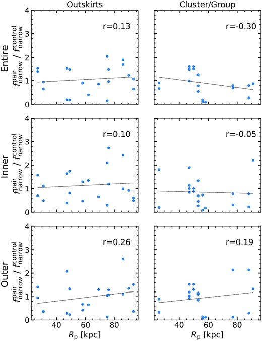
The kinematically narrow H i gas fractions (fnarrow) of the galaxy pairs normalized by fnarrow of the control galaxies at similar H i mass (|$f_{\rm {narrow}}^{\rm pair}$|/|$f_{\rm {narrow}}^{\rm control}$|) against the projected separation between the pairs for the entire, inner, and outer disc regions in the outskirts (left-hand panel) and cluster/group environments (right-hand panel). Linear regressions are indicated by the solid lines. The Pearson correlation coefficients r are shown in the top-right corner of each panel.
As shown in Fig. 12, no clear correlations between Rp and normalized fnarrow are found for the galaxy pairs in the environments given their Pearson correlation coefficients. However, the relations could be also affected by other galaxy properties like the stellar-mass ratio between pairs. Das et al. (2021) show that SFRs tend to be enhanced with decreasing Rp for SDSS galaxy pairs which have stellar mass ratio of 1< M1/M2 <3 where M1 and M2 are the stellar masses of the primary and secondary galaxies. On the other hand, the SFRs are likely to be suppressed in the ones with stellar mass ratios of 3< M1/M2 <10. No sign of correlations between normalized fnarrow and Rp and their large scatter shown in Fig. 12 for the paired galaxies could be attributed to the effect of their stellar-mass ratios.
4.3 Gravitational instability of the gas disc
In this section, we examine the influence of galaxy environments associated with the infall stage of galaxies (i.e. clusters, groups, pairs, and outskirts) on the gravitational instability of their gas discs. To quantify the degree of gravitational instability in the sample galaxies’ gas discs, we use the Toomre Q parameter value, which allows us to measure gas instability against gravitational collapse and SF. This is described in Section 3.4.
The estimation of the Toomre Q parameter is only valid for galaxies for which rotation curves are available. We therefore restrict our Toomre Q parameter analysis to the sample galaxies that show a clear rotation pattern in their single Gaussian fitting velocity fields and that have inclination values of 30° < i < 70° and resolved with more than ≥6 beams across their major axes. In addition, as mentioned in Section 3.2, for the galaxies whose single Gaussian fitting velocity field maps have large blank areas, we use their SoFiA2 moment1 maps. Typically, the percentage of masked pixels is less than 40|${{\ \rm per\ cent}}$| but with two exceptions, over about 50|${{\ \rm per\ cent}}$| are masked. These are indicated by ‘*’ in Table A1–A6.
There are 65 control galaxies and 12 galaxy pairs in the Hydra I, Norma, and NGC 4636 fields whose Toomre Q parameter values can be measured from the rotation curve analysis. For each galaxy, we derive median values of the Toomre Q parameters measured in the inner and outer gas disc regions, as well as in the entire one, as described in Section 3.4. The distribution of the Toomre Q parameter median values for the disc regions (inner, outer, and entire) of the sample galaxies in the different environments (outskirts, infall, and central) are presented in the upper panels of Fig. 13. The additional cuts for H i masses of galaxies and galaxy number ratios described in Section 2.3 result in 21 control galaxies and 7 paired galaxies. Their Toomre Q parameter distributions are shown in the lower panels of Fig. 13.
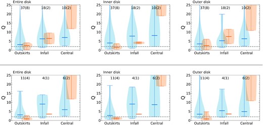
The Toomre Q parameter median values for the three different regions (‘Entire’, ‘Inner’, and ‘Outer’) of the sample galaxies that are not matched (upper panels) and matched (lower panels) in H i mass and galaxy number ratios, respectively, in the outskirts, infalling, and central environments. The control galaxies and galaxy pairs are shown with blue and orange colours, respectively. The numbers of the control and pair (bracket) galaxies are shown in each panel. The border thickness represents the relative frequency of the sample galaxies with the corresponding Toomre Q parameter median values. The small horizontal lines in each panel indicate the median values. The grey horizontal dashed lines indicate the Q = 2 values. See Section 4.3 for more details.
As shown in the upper panels of Fig. 13, the median values of the Toomre Q parameters of all the control galaxies are the lowest (more unstable) and highest (more stable) in the outskirts and central environments, respectively. Largely, this trend holds for the three gas disc regions (inner, outer, and entire) although the distribution tails for outskirts and central galaxies are further extended towards higher Q values up to 60.4. The central environment with a higher local density of galaxies and IGM could result in such higher Q values for the central galaxies in a way of increasing their gas velocity dispersions (See equation 7). Galaxies in central environments are likely to be more affected by gravitational and/or hydrodynamical influences, including ram pressure stripping, galaxy–galaxy interactions, and gas accretion than infalling and outskirts galaxies. These all might have given rise to turbulent gas motions in their gas discs (Gunn & Gott 1972; Moore et al. 1996; Park & Hwang 2009; Wong et al. 2014; Yoon et al. 2017).
Despite the small number of statistics, the trend of the higher Toomre Q values for the galaxies in the central environment is also seen for the galaxy pairs. The higher Q values of the galaxy pairs in the central environment could be also attributed by the aforementioned dynamical effects like ram pressure stripping and tidal interactions among galaxies. External gravitational and/or hydrodynamical effects in the central environment might be associated with the higher Toomre Q values. Alternatively, internal processes (e.g. SF and feedback) of the galaxies could also have disturbed the gas motions, resulting in the higher Toomre Q values. However, we note that the H i masses of the galaxies and the galaxy number ratios in the environments are not matched. The trend of increasing Toomre Q parameter values towards the central environment could be biased by the unmatched sample.
The distributions of the Toomre Q parameters of the matched control galaxies are shown in the lower panels of Fig. 13. The median values for the three regions (entire, inner, and outer discs) of the control galaxies (blue) in the infall and central environments are higher than those of the galaxies in the outskirts environment. However, it is difficult to see whether this trend is present for the matched galaxy pairs (orange) due to the limited number of galaxies.
We point out that the Toomre Q analysis of the sample galaxies could be affected by resolution effects. If the beam resolution was not high enough to resolve the inner regions of our sample galaxies where velocity gradients are high, their gas velocity dispersions could be overestimated. In addition, rotation velocities of galaxies with steeply rising rotation curves are prone to be underestimated at low-angular resolutions. 2D tilted-ring analysis is usually affected by this so-called beam smearing effect. Inaccurate measurements (i.e. R/V and dV/dR) of the rotation curve shape of a galaxy, particularly in the inner region, will lead to uncertainties in the Toomre Q parameter analysis. This could result in the wider distribution of the Toomre Q parameter values for the inner disc region than those for the outer disc of the control galaxies in the infalling and central environments in Fig. 13. This demonstrates the need for higher angular resolution H i observations not only to minimize beam smearing effects but also to improve the small number of statistics in the Toomre Q parameter analysis of this work. We tabulate the values for the median and standard deviation of the Toomre Q parameter values derived for the entire, inner, and outer gas discs of the sample galaxies in Table 4.
4.4 Morphological H i asymmetries
In this section, we examine morphological disturbances of the gas distribution of the sample galaxies in different galaxy environments. H i gas in galaxies usually extends further than the readily discernible stellar disc and thus is a useful probe of environmental effects (Westmeier, Braun & Koribalski 2011; Odekon et al. 2016; Yoon et al. 2017). Several hydrodynamical processes in and around galaxies (internal: spiral arms and bars; external: ram pressure stripping, minor or major mergers, tidal interactions, and gas accretion) are able to disturb the gas distribution, particularly in the outer region, which increases morphological H i asymmetries of the gas discs (Gunn & Gott 1972; Mapelli, Moore & Bland-Hawthorn 2008; Holwerda et al. 2011; Reynolds et al. 2020; Watts et al. 2020a, b). As described in Section 3.5, to quantify the morphological H i disturbances of galaxies in our sample, we measure H i asymmetries using their integrated intensity maps (moment0). We exclude four galaxy pairs and 13 control galaxies that are not well resolved spatially and thus whose kinematic centres are not reliably derived. Fig. 14 shows the derived H i asymmetries of the selected galaxies in the three galaxy environments.
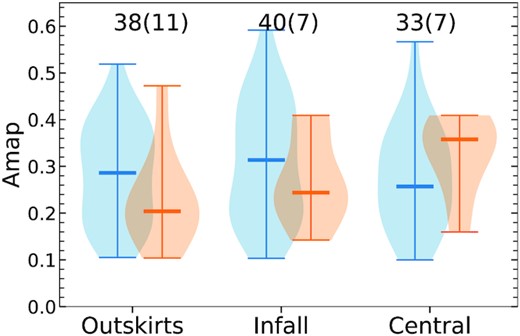
The H i morphological asymmetries of the sample galaxies, in the outskirts, infalling, and central environments. The control galaxies and galaxy pairs are shown with blue and orange colours, respectively. The numbers of the control and pair (bracket) galaxies are shown in each panel. The border thickness represents the relative frequency of the sample galaxies with the corresponding H i morphological asymmetries. The small horizontal lines in each panel indicate the median values. See Section 4.4 for more details.
As discussed in Reynolds et al. (2021) and Wang et al. (2021), the effect of ram pressure stripping on the galaxies in the Hydra I cluster could affect their H i asymmetries in a way of that gives rise to morphological disturbances. Additionally, external tidal forces from other galaxies in the central environment might have disturbed their H i gas distribution, resulting in complex H i gas structures (e.g. H i tails or streams) and kinematics, particularly in their outer regions where the gravitational potential is shallow. This can also apply to the Norma cluster and the NGC 4636 galaxies in dense environments. In this respect, environmental effects, including ram pressure stripping, on the H i asymmetry of a galaxy are expected to be minimal in the outskirts environment.
In Fig. 14, no clear trend in the median values of the H i asymmetries (|$A_{\rm {map}}^{\rm {H\, \small {\rm I}}}$|) of the control sample galaxies (blue) is found with respect to the environments (outskirts to central). On the other hand, the median |$A_{\rm {map}}^{\rm {H\, \small {\rm I}}}$| value (0.20) of the galaxy pairs (orange) in the outskirts is slightly smaller than those (0.24 and 0.36) of the pairs in the infalling and central environments. Reynolds et al. (2021) derive the |$A_{\rm {map}}^{\rm {H\, \small {\rm I}}}$| value of a galaxy in a way of minimizing it by varying the mass centre of the moment0 map within one ASKAP beam size. However, we fix the centre in equation (10) with the value determined from the 2dbat analysis when deriving |$A_{\rm {map}}^{\rm {H\, \small {\rm I}}}$|. So the H i asymmetry values of the galaxy pairs in the infalling and central environments could potentially be increased by the way of asymmetry measurement adopted in this work.
More importantly, as discussed in Giese et al. (2016; see also Reynolds et al. 2020, 2021), the measurement of morphological H i asymmetries of galaxies using equation (10) is not reliable for H i observations at low spatial resolutions and with low S/N. Additionally, the current sensitivity of ASKAP pilot observations may not be high enough to detect, if any, signatures of H i morphological disturbances in the outer regions of the galaxy pairs in the outskirts (see also Reynolds et al. 2021). This demonstrates the need for deeper H i observations in different environments at high sensitivities, as well as at high-angular resolutions, in order to better examine the environmental effects on the morphological H i asymmetries of galaxies. We list the median values and standard deviations of the derived H i asymmetries of the sample galaxies in Table 5.
The median values (|$\langle A_{\rm {map}}^{\rm {H\, \small {\rm I}}} \rangle ^{\rm {median}}$|) and standard deviations (|$\sigma _{A_{\rm {map}}^{\rm {H\, \small {\rm I}}}}$|) of the morphological H i asymmetries of the galaxy pairs and control sample galaxies in the outskirts, infalling, and central environments. N is the number of samples, and CI denotes the 95|${{\ \rm per\ cent}}$| confidence interval for median value.
| Outskirts | Infalling | Central | ||||||||||
|---|---|---|---|---|---|---|---|---|---|---|---|---|
| |$\langle A_{\rm {map}}^{\rm {H\, \small {\rm I}}} \rangle ^{\rm {median}}$| | 1σ | CI | N | |$\langle A_{\rm {map}}^{\rm {H\, \small {\rm I}}} \rangle ^{\rm {median}}$| | 1σ | CI | N | |$\langle A_{\rm {map}}^{\rm {H\, \small {\rm I}}} \rangle ^{\rm {median}}$| | 1σ | CI | N | |
| Control | 0.29 | 0.11 | (0.23, 0.35) | 38 | 0.31 | 0.13 | (0.24, 0.39) | 40 | 0.26 | 0.11 | (0.21, 0.34) | 33 |
| Pair | 0.20 | 0.10 | (0.18, 0.33) | 11 | 0.24 | 0.09 | – | 7 | 0.36 | 0.08 | – | 7 |
5 SUMMARY
In this paper, we examine the galaxy environmental effects on the resolved H i properties of galaxy pairs in the two clusters (Hydra I and Norma) and the galaxy group (NGC 4636) from the ASKAP pilot observations. We perform profile decomposition of the H i data cubes using a new tool, baygaud, which allows us to deblend a line-of-sight velocity profile with an optimal number of Gaussian components based on Bayesian nested sampling. Then, we construct H i superprofiles via stacking individual line profiles after aligning their centroid velocities. We fit the H i superprofiles with a double Gaussian model and classify them as kinematically narrow and broad H i gas components with respect to their velocity dispersions, i.e. having narrower and broader σ, respectively. The kinematically narrow H i gas components can be associated with cool H i gas (Ianjamasimanana et al. 2012). Additionally, we quantify the gravitational instability of the H i gas disc of galaxy pairs using their Toomre Q parameters, and H i morphological disturbances. For this, we use their moment0 maps produced by SoFiA2. These H i properties are then compared with those of a set of control galaxies which are classified as non-paired systems in the same fields.
We investigate the cluster environmental effects on the H i gas properties of galaxy pairs by comparing H i superprofiles, Toomre Q parameter values, and morphological asymmetries in three different environments: (1) outskirts, (2) infalling, and (3) central, which are defined using the phase-space diagrams of the galaxy clusters and group. The main results of this paper are as follows:
The median value of fnarrow (|$M_{\rm {narrow}}^{\rm {H\, \small {\rm I}}}$| / |$M_{\rm {total}}^{\rm {H\, \small {\rm I}}}$|) for the outer gas disc regions of the control sample galaxies appears to be lower in the central environment than outskirts and infalling environments. This could be attributed to the enhanced local densities of galaxies in the central environment. Tidal interactions among galaxies in denser environments can give rise to more turbulent gas motions in the galaxies with higher velocity dispersions. Together, the ram pressure induced by the IGM in the clusters may also contribute to decrease fnarrow in a way of stripping part of the kinematically narrow H i gas in the outer regions of the galaxies (Chung et al. 2009; Cortese et al. 2011; Jaffé et al. 2016; Brown et al. 2017). Despite the small number statistics, a decreasing trend offnarrow values for the galaxy pairs is seen with the infalling stage, outskirts to central, particularly in their outer gas disc regions. This tendency is also seen in the inner gas disc regions but is less significant, possibly due to the higher gravitational potential. Tidal interactions of galaxies in the close galaxy pairs in denser environments could have induced such a tendency, giving rise to more turbulent gas motions. The lower fnarrow values of the galaxy pairs in denser environments are consistent with the results from other works that galaxy pairs in low-density environments tend to have high SF rates caused by higher gas fractions (Ellison et al. 2010).
Despite a wide range of the Toomre Q parameter values and the small number of statistics, the median values for the control galaxies are likely to increase (i.e. being more stable) in denser environments. This tendency is further enhanced for the galaxy pairs. The increased kinetic energy which is possibly caused by the ram pressure stripping and/or tidal interactions in the central environment might have stirred up the gas in the galaxies, making the gas discs of the galaxies more stable against gravitational collapse.
The median value of the H i morphological asymmetries (|$A_{\rm {map}}^{\rm {H\, \small {\rm I}}}$|) of the control galaxies is the lowest in the central environment but it is not significant. On the other hand, the median values of |$A_{\rm {map}}^{\rm {H\, \small {\rm I}}}$| of the galaxy pairs increase towards the denser environments (outskirts to central). External processes like tidal interactions and ram pressure stripping in the central environment might have led to disturbed H i gas structures (e.g. H i tails or streams) in the outer gas discs of the galaxies. However, the current sensitivity and beam resolution of the ASKAP pilot observations may not be high enough to detect such disturbed H i features in the outer regions of the galaxies (Wang et al. 2021; Reynolds et al. 2022). The |$A_{\rm {map}}^{\rm {H\, \small {\rm I}}}$| values derived in our work could suffer from resolution effects, as discussed in Giese et al. (2016) and Reynolds et al. (2020), Reynolds et al. (2021). Deeper H i observations of the cluster and group galaxies to better sensitivity are needed in order to examine the environmental effects on their H i morphological disturbances.
SUPPORTING INFORMATION
ASKAP_galaxy_pairs_Supplementary_Material_2nd.pdf
Please note: Oxford University Press is not responsible for the content or functionality of any supporting materials supplied by the authors. Any queries (other than missing material) should be directed to the corresponding author for the article.
ACKNOWLEDGEMENTS
SHOH acknowledges a support from the National Research Foundation of Korea (NRF) grant funded by the Korea government (Ministry of Science and ICT: MSIT; No. NRF-2020R1A2C1008706). PK is partially supported by the BMBF project 05A17PC2 for D-MeerKAT. Parts of this research were conducted by the Australian Research Council Centre of Excellence for All Sky Astrophysics in 3 Dimensions (ASTRO 3D), through project number CE170100013. FB acknowledges funding from the European Research Council (ERC) under the European Union’s Horizon 2020 research and innovation programme (grant agreement no.726384/Empire).
DATA AVAILABILITY
The galaxy properties used in this work are available as online supplementary material. We show the first four rows of the tables for the H i properties and distances and representative two images and superprofiles of sample galaxies in Appendix A. The 30 arcsec H i data cubes and associated moment maps are available from the CSIRO ASKAP Science Data Archive (CASDA; Chapman 2015; Huynh et al. 2020) with the doi https://doi.org/10.25919/5f7bde37c20b5.
Footnotes
The Sloan Digital Sky Survey (SDSS) (York et al. 2000).
Cosmic Flows (Courtois et al. 2011).
The 6dF Galaxy Survey (6dFGS) (Beutler et al. 2011).
The HI Parkes All Sky Survey (HIPASS) (Barnes et al. 2001).
The HI Nearby Galaxy Survey (Walter et al. 2008).
Local Irregulars That Trace Luminosity Extremes, The HI Nearby Galaxy Survey (LITTLE THINGS) (Hunter et al. 2012).
REFERENCES
APPENDIX A: H i PROPERTIES, IMAGES, AND SUPERPROFILES OF THE SAMPLE GALAXIES
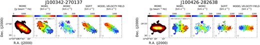
H i images of the galaxy pairs (ordered by the WALLABY ID) in the ASKAP Hydra I cluster field: ‘MOM0’ (SoFiA2 integrated intensity map, moment0), ‘MOM1’ (SoFiA2 velocity field map, moment1), ‘MOM2’ (SoFiA2, velocity dispersion map, moment2), SGFIT (baygaud Single Gaussian fitting (SGfit) velocity field map), and ‘MODEL VELOCITY FIELD’ (2dbat model velocity field map). The contour levels for each velocity field are denoted in the second panel of each figure. The ASKAP beam is shown as an ellipse on the bottom-left corner of each panel. The full figure is provided with supplementary material.
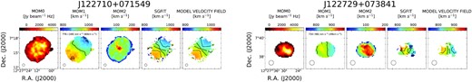
H i images of the galaxy pairs (ordered by the WALLABY ID) in the ASKAP NGC 4636 field: ‘MOM0’ (SoFiA2 integrated intensity map, moment0), ‘MOM1’ (SoFiA2 velocity field map, moment1), ‘MOM2’ (SoFiA2, velocity dispersion map, moment2), SGFIT (baygaud Single Gaussian fitting (SGfit) velocity field map), and ‘MODEL VELOCITY FIELD’ (2dbat model velocity field map). The contour levels for each velocity field are denoted in the second panel of each figure. The ASKAP beam is shown as an ellipse on the bottom-left corner of each panel. The full figure is provided with supplementary material.

H i images of the galaxy pairs (ordered by the WALLABY ID) in the ASKAP Norma cluster field: ‘MOM0’ (SoFiA2 integrated intensity map, moment0), ‘MOM1’ (SoFiA2 velocity field map, moment1), ‘MOM2’ (SoFiA2, velocity dispersion map, moment2), SGFIT (baygaud Single Gaussian fitting (SGfit) velocity field map), and ‘MODEL VELOCITY FIELD’ (2dbat model velocity field map). The contour levels for each velocity field are denoted in the second panel of each figure. The ASKAP beam is shown as an ellipse on the bottom-left corner of each panel. The full figure is provided with supplementary material.
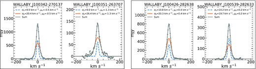
baygaud based H i superprofiles of the galaxy pairs (ordered by the WALLABY ID) in the ASKAP Hydra I cluster field. The grey circles show the stacked fluxes at the corresponding channels. The blue-dashed and orange-solid lines represent the narrow and broad components decomposed from the double Gaussian fitting to the superprofiles. Their velocity dispersions (σ) and centroid velocities (μ) are labelled on the top-right corner of each panel. H i superprofiles of galaxies which are poorly resolved are blanked. The full figure is provided with supplementary material.
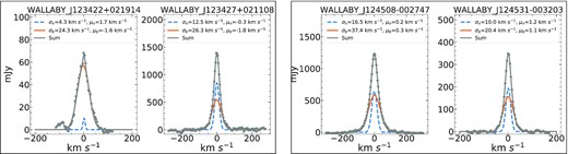
baygaud based H i superprofiles of the galaxy pairs (ordered by the WALLABY ID) in the ASKAP NGC 4636 group field. The grey circles show the stacked fluxes at the corresponding channels. The blue-dashed and orange-solid lines represent the narrow and broad components decomposed from the double Gaussian fitting to the superprofiles. Their velocity dispersions (σ) and centroid velocities (μ) are labelled on the top-right corner of each panel. H i superprofiles of galaxies which are poorly resolved are blanked. The full figure is provided with supplementary material.
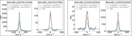
baygaud based H i superprofiles of the galaxy pairs (ordered by the WALLABY ID) in the ASKAP Norma cluster field. The grey circles show the stacked fluxes at the corresponding channels. The blue-dashed and orange-solid lines represent the narrow and broad components decomposed from the double Gaussian fitting to the superprofiles. Their velocity dispersions (σ) and centroid velocities (μ) are labelled on the top-right corner of each panel. H i superprofiles of galaxies that are poorly resolved are blanked. The full figure is provided with supplementary material.
H i properties and distances of the control galaxies in the ASKAP Hydra I cluster field. The full table is provided with supplementary material.
| Name | RA (J2000) | Dec. (J2000) | D | Vsys | |$R_{rm{H\, \small {\rm I}}}$| | |$S_{rm{H\, \small {\rm I}}}$| | |$M_{\rm {total}}^{rm{H\, \small {\rm I}}}$| | |$M_{\rm {narrow}}^{rm{H\, \small {\rm I}}}$| | |$M_{\rm {broad}}^{rm{H\, \small {\rm I}}}$| | |$A_{\rm {map}}^{rm{H\, \small {\rm I}}}$| | Q |
|---|---|---|---|---|---|---|---|---|---|---|---|
| (Mpc) | (|$\mathrm{km}\, \mathrm{s}^{-1}$|) | (kpc) | (Jy km s−1) | (|$10^8 \ \rm {M_{\odot }}$|) | (|$10^8 \ \rm {M_{\odot }}$|) | (|$10^8 \ \rm {M_{\odot }}$|) | |||||
| (1) | (2) | (3) | (4) | (5) | (6) | (7) | (8) | (9) | (10) | (11) | (12) |
| J100351-273417 | 10|$^{\rm {h}}03^{\rm {m}}52.\hskip-2.3pt^{\rm {s}}$|0 | |$-27^{\rm {d}}34^{\rm {m}}15.\hskip-2.3pt^{\rm {s}}$|3 | 39.9 | 2,792 | 30.5 | 12.6 | 47.2 | 12.4 | 34.8 | 0.23 | 4.22 |
| J100634-295615 | 10|$^{\rm {h}}06^{\rm {m}}34.\hskip-2.3pt^{\rm {s}}$|2 | |$-29^{\rm {d}}56^{\rm {m}}12.\hskip-2.3pt^{\rm {s}}$|2 | 15.9 | 1,117 | 9.6 | 9.2 | 5.5 | 1.3 | 4.2 | 0.23 | 10.21 |
| J100656-251731† | 10|$^{\rm {h}}06^{\rm {m}}55.\hskip-2.3pt^{\rm {s}}$|9 | |$-25^{\rm {d}}17^{\rm {m}}32.\hskip-2.3pt^{\rm {s}}$|5 | 41.3 | 2,894 | 10.5 | 1.6 | 6.5 | 3.0 | 3.5 | 0.27 | … |
| J100713-262336 | 10|$^{\rm {h}}07^{\rm {m}}13.\hskip-2.3pt^{\rm {s}}$|8 | |$-26^{\rm {d}}23^{\rm {m}}31.\hskip-2.3pt^{\rm {s}}$|4 | 65.7 | 4,599 | 17.1 | 2.0 | 20.5 | 16.8 | 3.7 | 0.21 | … |
The columns are (1) source name; (2) kinematic centre in RA units from 2dbat; (3) kinematic centre Dec. units from 2dbat; (4) distance to the galaxy from redshift (Mpc); (5) systemic velocity from redshift (|$\mathrm{km}\, \mathrm{s}^{-1}$|) ; (6) radius of H i disc from the baygaud analysis, |$R_{rm{H\, \small {\rm I}}}$| (kpc); (7) integrated H i intensities derived from superprofiles in Section 3 (Jy km s−1); (8) H i mass derived from superprofiles in Section 3 (|$10^8 \ \rm {M_{\odot }}$|); (9) narrow H i mass derived from superprofiles in Section 3 (|$10^8 \ \rm {M_{\odot }}$|); (10) broad H i mass derived from superprofiles in Section 3 (|$10^8 \ \rm {M_{\odot }}$|); (11) H i morphological asymmetry of the galaxy; (12) median values of the Toomre Q parameter values of the galaxy. ‘†’ indicates the galaxy that have similar velocity widths of the narrow and broad components in the H i superprofile analysis.
H i properties and distances of the paired galaxies in the ASKAP Hydra I cluster field. The full table is provided with supplementary material.
| Name | RA (J2000) | Dec. (J2000) | D | Vsys | |$R_{rm{H\, \small {\rm I}}}$| | |$S_{rm{H\, \small {\rm I}}}$| | |$M_{\rm {total}}^{rm{H\, \small {\rm I}}}$| | |$M_{\rm {narrow}}^{rm{H\, \small {\rm I}}}$| | |$M_{\rm {broad}}^{rm{H\, \small {\rm I}}}$| | Rp | ΔV | |$A_{\rm {map}}^{rm{H\, \small {\rm I}}}$| | Q |
|---|---|---|---|---|---|---|---|---|---|---|---|---|---|
| (Mpc) | (|$\mathrm{km}\, \mathrm{s}^{-1}$|) | (kpc) | (Jy km s−1) | (|$10^8 \ \rm {M_{\odot }}$|) | (|$10^8 \ \rm {M_{\odot }}$|) | (|$10^8 \ \rm {M_{\odot }}$|) | (kpc) | (|$\mathrm{km}\, \mathrm{s}^{-1}$|) | |||||
| (1) | (2) | (3) | (4) | (5) | (6) | (7) | (8) | (9) | (10) | (11) | (12) | (13) | (14) |
| J100336-262923 | 10|$^{\rm {h}}03^{\rm {m}}37.\hskip-2.3pt^{\rm {s}}$|4 | |$-26^{\rm {d}}29^{\rm {m}}39.\hskip-2.3pt^{\rm {s}}$|1 | 12.9 | 901 | 4.3 | 1.8 | 0.7 | 0.2 | 0.5 | 31 | 26 | … | … |
| J100342-270137 | 10|$^{\rm {h}}03^{\rm {m}}41.\hskip-2.3pt^{\rm {s}}$|9 | |$-27^{\rm {d}}01^{\rm {m}}39.\hskip-2.3pt^{\rm {s}}$|5 | 13.7 | 957 | 15.5 | 45.7 | 20.2 | 6.8 | 13.3 | 93 | 83 | 0.09 | 2.46 |
| J100351-263707 | 10|$^{\rm {h}}03^{\rm {m}}51.\hskip-2.3pt^{\rm {s}}$|9 | |$-26^{\rm {d}}36^{\rm {m}}35.\hskip-2.3pt^{\rm {s}}$|5 | 12.5 | 874 | 6.6 | 6.7 | 2.4 | 0.5 | 1.9 | 31/93 | 26/83 | … | … |
| J100426-282638 | 10|$^{\rm {h}}04^{\rm {m}}26.\hskip-2.3pt^{\rm {s}}$|3 | |$-28^{\rm {d}}26^{\rm {m}}40.\hskip-2.3pt^{\rm {s}}$|8 | 15.5 | 1,083 | 15.6 | 32.4 | 18.3 | 4.9 | 13.3 | 69 | 41 | 0.10 | 2.70 |
Note. The columns are (1) source name; (2) kinematic centre in RA units from 2dbat; (3) kinematic centre Dec. units from 2dbat; (4) distance to the galaxy from redshift (Mpc); (5) systemic velocity from redshift (|$\mathrm{km}\, \mathrm{s}^{-1}$|) ; (6) radius of H i disc from the baygaud analysis, |$R_{rm{H\, \small {\rm I}}}$| (kpc); (7) integrated H i intensities derived from superprofiles in Section 3 (Jy km s−1); (8) H i mass derived from superprofiles in Section 3 (|$10^8 \ \rm {M_{\odot }}$|); (9) narrow H i mass derived from superprofiles in Section 3 (|$10^8 \ \rm {M_{\odot }}$|); (10) broad H i mass derived from superprofiles in Section 3 (|$10^8 \ \rm {M_{\odot }}$|); (11) projected distance to the companion galaxy (kpc). For galaxies with two nearby companions, we provide two Rp values separated by ‘/’; (12) relative line-of-sight velocity to the companion galaxy (|$\mathrm{km}\, \mathrm{s}^{-1}$|) . For galaxies with two nearby companions, we provide two ΔV values separated by ‘/’; (13) H i morphological asymmetry of the galaxy; (14) median values of the Toomre Q parameter values of the galaxy. ‘*’ indicates the visually identified galaxy pair. ‘†’ indicates the galaxy that have similar velocity widths of the narrow and broad components in the H i superprofile analysis.
H i properties and distances of the control galaxies in the ASKAP NGC 4636 field. The full table is provided with supplementary material.
| Name | RA (J2000) | Dec. (J2000) | D | Vsys | |$R_{rm{H\, \small {\rm I}}}$| | |$S_{rm{H\, \small {\rm I}}}$| | |$M_{\rm {total}}^{rm{H\, \small {\rm I}}}$| | |$M_{\rm {narrow}}^{rm{H\, \small {\rm I}}}$| | |$M_{\rm {broad}}^{rm{H\, \small {\rm I}}}$| | |$A_{\rm {map}}^{rm{H\, \small {\rm I}}}$| | Q |
|---|---|---|---|---|---|---|---|---|---|---|---|
| (Mpc) | (|$\mathrm{km}\, \mathrm{s}^{-1}$|) | (kpc) | (Jy km s−1) | (|$10^8 \ \rm {M_{\odot }}$|) | (|$10^8 \ \rm {M_{\odot }}$|) | (|$10^8 \ \rm {M_{\odot }}$|) | |||||
| (1) | (2) | (3) | (4) | (5) | (6) | (7) | (8) | (9) | (10) | (11) | (12) |
| J122708+055255 | 12|$^{\rm {h}}27^{\rm {m}}09.\hskip-2.3pt^{\rm {s}}$|3 | +05|$^{\rm {d}}52^{\rm {m}}50.\hskip-2.3pt^{\rm {s}}$|6 | 15.9 | 1,113 | 9.9 | 11.2 | 6.7 | 5.7 | 1.0 | 0.40 | 4.00 |
| J122755+054312 | 12|$^{\rm {h}}27^{\rm {m}}55.\hskip-2.3pt^{\rm {s}}$|5 | +05|$^{\rm {d}}43^{\rm {m}}14.\hskip-2.3pt^{\rm {s}}$|8 | 32.0 | 2,243 | 5.3 | 1.2 | 2.8 | 0.4 | 2.4 | 0.19 | … |
| J122928+064623 | 12|$^{\rm {h}}29^{\rm {m}}28.\hskip-2.3pt^{\rm {s}}$|6 | +06|$^{\rm {d}}46^{\rm {m}}12.\hskip-2.3pt^{\rm {s}}$|0 | 7.5 | 527 | 2.3 | 3.6 | 0.5 | 0.1 | 0.4 | 0.41 | … |
| J122930+074142 | 12|$^{\rm {h}}29^{\rm {m}}30.\hskip-2.3pt^{\rm {s}}$|5 | +07|$^{\rm {d}}41^{\rm {m}}46.\hskip-2.3pt^{\rm {s}}$|8 | 10.7 | 748 | 3.0 | 1.5 | 0.4 | 0.1 | 0.3 | 0.22 | … |
Note. The columns are (1) source name; (2) kinematic centre in RA units from 2dbat; (3) kinematic centre Dec. units from 2dbat; (4) distance to the galaxy from redshift (Mpc); (5) systemic velocity from redshift (|$\mathrm{km}\, \mathrm{s}^{-1}$|) ; (6) radius of H i disc from the baygaud analysis, |$R_{rm{H\, \small {\rm I}}}$| (kpc); (7) integrated H i intensities derived from superprofiles in Section 3 (Jy km s−1); (8) H i mass derived from superprofiles in Section 3 (|$10^8 \ \rm {M_{\odot }}$|); (9) narrow H i mass derived from superprofiles in Section 3 (|$10^8 \ \rm {M_{\odot }}$|); (10) broad H i mass derived from superprofiles in Section 3 (|$10^8 \ \rm {M_{\odot }}$|); (11) H i morphological asymmetry of the galaxy, (12) median values of the Toomre Q parameter values of the galaxy (‘*’: moment1 velocity field is used for the rotation curve analysis).
H i properties and distances of the paired galaxies in the ASKAP NGC 4636 field. The full table is provided with supplementary material.
| Name | RA (J2000) | Dec. (J2000) | D | Vsys | |$R_{rm{H\, \small {\rm I}}}$| | |$S_{rm{H\, \small {\rm I}}}$| | |$M_{\rm {total}}^{rm{H\, \small {\rm I}}}$| | |$M_{\rm {narrow}}^{rm{H\, \small {\rm I}}}$| | |$M_{\rm {broad}}^{rm{H\, \small {\rm I}}}$| | Rp | ΔV | |$A_{\rm {map}}^{rm{H\, \small {\rm I}}}$| | Q |
|---|---|---|---|---|---|---|---|---|---|---|---|---|---|
| (Mpc) | (|$\mathrm{km}\, \mathrm{s}^{-1}$|) | (kpc) | (Jy km s−1) | (|$10^8 \ \rm {M_{\odot }}$|) | (|$10^8 \ \rm {M_{\odot }}$|) | (|$10^8 \ \rm {M_{\odot }}$|) | (kpc) | (|$\mathrm{km}\, \mathrm{s}^{-1}$|) | |||||
| (1) | (2) | (3) | (4) | (5) | (6) | (7) | (8) | (9) | (10) | (11) | (12) | (13) | (14) |
| J122710+071549 | 12|$^{\rm {h}}27^{\rm {m}}11.\hskip-2.3pt^{\rm {s}}$|3 | +07|$^{\rm {d}}15^{\rm {m}}49.\hskip-2.3pt^{\rm {s}}$|2 | 13.3 | 929 | 11.3 | 21.1 | 8.8 | 4.7 | 4.0 | 86 | 68 | 0.20 | … |
| J122729+073841 | 12|$^{\rm {h}}27^{\rm {m}}29.\hskip-2.3pt^{\rm {s}}$|4 | +07|$^{\rm {d}}38^{\rm {m}}48.\hskip-2.3pt^{\rm {s}}$|4 | 12.3 | 860 | 4.6 | 3.5 | 1.3 | 0.8 | 0.5 | 86 | 68 | 0.36 | … |
| J123422+021914 | 12|$^{\rm {h}}34^{\rm {m}}21.\hskip-2.3pt^{\rm {s}}$|8 | +02|$^{\rm {d}}19^{\rm {m}}25.\hskip-2.3pt^{\rm {s}}$|3 | 25.4 | 1,779 | 7.5 | 3.5 | 5.4 | 0.2 | 5.2 | 58 | 19 | … | … |
| J124508-002747 | 12|$^{\rm {h}}45^{\rm {m}}08.\hskip-2.3pt^{\rm {s}}$|4 | |$-00^{\rm {d}}27^{\rm {m}}47.\hskip-2.3pt^{\rm {s}}$|4 | 21.9 | 1,534 | 34.3 | 80.5 | 91.2 | 30.0 | 61.2 | 47 | 84 | 0.17 | 9.51 |
Note. The columns are (1) source name; (2) kinematic centre in RA units from 2dbat; (3) kinematic centre Dec. units from 2dbat; (4) distance to the galaxy from redshift (Mpc); (5) systemic velocity from redshift (|$\mathrm{km}\, \mathrm{s}^{-1}$|) ; (6) radius of H i disc from the baygaud analysis, |$R_{rm{H\, \small {\rm I}}}$| (kpc); (7) integrated H i intensities derived from superprofiles in Section 3 (Jy km s−1); (8) H i mass derived from superprofiles in Section 3 (|$10^8 \ \rm {M_{\odot }}$|); (9) narrow H i mass derived from superprofiles in Section 3 (|$10^8 \ \rm {M_{\odot }}$|); (10) broad H i mass derived from superprofiles in Section 3 (|$10^8 \ \rm {M_{\odot }}$|); (11) projected distance to the companion galaxy (kpc). For galaxies with two nearby companions, we provide two Rp values separated by ‘/’; (12) relative line-of-sight velocity to the companion galaxy (|$\mathrm{km}\, \mathrm{s}^{-1}$|) . For galaxies with two nearby companions, we provide two ΔV values separated by ‘/’; (13) H i morphological asymmetry of the galaxy; (14) median values of the Toomre Q parameter of the galaxy.
H i properties and distances of the control galaxies in the ASKAP Norma cluster field. The full table is provided with supplementary material.
| Name | RA (J2000) | Dec. (J2000) | D | Vsys | |$R_{rm{H\, \small {\rm I}}}$| | |$S_{rm{H\, \small {\rm I}}}$| | |$M_{\rm {total}}^{rm{H\, \small {\rm I}}}$| | |$M_{\rm {narrow}}^{rm{H\, \small {\rm I}}}$| | |$M_{\rm {broad}}^{rm{H\, \small {\rm I}}}$| | |$A_{\rm {map}}^{rm{H\, \small {\rm I}}}$| | Q |
|---|---|---|---|---|---|---|---|---|---|---|---|
| (Mpc) | (|$\mathrm{km}\, \mathrm{s}^{-1}$|) | (kpc) | (Jy km s−1) | (|$10^8 \ \rm {M_{\odot }}$|) | (|$10^8 \ \rm {M_{\odot }}$|) | (|$10^8 \ \rm {M_{\odot }}$|) | |||||
| (1) | (2) | (3) | (4) | (5) | (6) | (7) | (8) | (9) | (10) | (11) | (12) |
| J163435-620248 | 16|$^{\rm {h}}34^{\rm {m}}34.\hskip-2.3pt^{\rm {s}}$|7 | |$-62^{\rm {d}}02^{\rm {m}}45.\hskip-2.3pt^{\rm {s}}$|3 | 63.6 | 4,450 | 28.4 | 5.2 | 49.4 | 10.8 | 38.5 | 0.14 | 3.14 |
| J163452-603705 | 16|$^{\rm {h}}34^{\rm {m}}52.\hskip-2.3pt^{\rm {s}}$|8 | -60|$^{\rm {d}}37^{\rm {m}}07.\hskip-2.3pt^{\rm {s}}$|8 | 46.7 | 3,266 | 32.5 | 15.1 | 77.5 | 18.3 | 59.2 | 0.15 | 0.03 |
| J163518-581311 | 16|$^{\rm {h}}35^{\rm {m}}19.\hskip-2.3pt^{\rm {s}}$|1 | -58|$^{\rm {d}}13^{\rm {m}}09.\hskip-2.3pt^{\rm {s}}$|0 | 22.3 | 1,562 | 13.4 | 10.6 | 12.4 | 1.3 | 11.2 | 0.24 | 4.55 |
| J163600-611510 | 16|$^{\rm {h}}36^{\rm {m}}00.\hskip-2.3pt^{\rm {s}}$|4 | |$-61^{\rm {d}}15^{\rm {m}}11.\hskip-2.3pt^{\rm {s}}$|2 | 75.8 | 5,307 | 16.3 | 1.3 | 17.4 | 11.9 | 5.5 | 0.32 | … |
Note. The columns are (1) source name; (2) kinematic centre in RA units from 2dbat; (3) kinematic centre Dec. units from 2dbat; (4) distance to the galaxy from redshift (Mpc); (5) systemic velocity from redshift (|$\mathrm{km}\, \mathrm{s}^{-1}$|) ; (6) radius of H i disc from the baygaud analysis, |$R_{rm{H\, \small {\rm I}}}$| (kpc); (7) integrated H i intensities derived from superprofiles in Section 3 (Jy km s−1); (8) H i mass derived from superprofiles in Section 3 (|$10^8 \ \rm {M_{\odot }}$|); (9) narrow H i mass derived from superprofiles in Section 3 (|$10^8 \ \rm {M_{\odot }}$|); (10) broad H i mass derived from superprofiles in Section 3 (|$10^8 \ \rm {M_{\odot }}$|); (11) H i morphological asymmetry of the galaxy; (12) median values of the Toomre Q parameter values of the galaxy (‘*’: moment1 velocity field is used for the rotation curve analysis). ‘†’ indicates the galaxy that have similar velocity widths of the narrow and broad components in the H i superprofile analysis.
H i properties and distances of the paired galaxies in the ASKAP Norma cluster field. The full table is provided with supplementary material.
| Name | RA (J2000) | Dec. (J2000) | D | Vsys | |$R_{rm{H\, \small {\rm I}}}$| | |$S_{rm{H\, \small {\rm I}}}$| | |$M_{\rm {total}}^{rm{H\, \small {\rm I}}}$| | |$M_{\rm {narrow}}^{rm{H\, \small {\rm I}}}$| | |$M_{\rm {broad}}^{rm{H\, \small {\rm I}}}$| | Rp | ΔV | |$A_{\rm {map}}^{rm{H\, \small {\rm I}}}$| | Q |
|---|---|---|---|---|---|---|---|---|---|---|---|---|---|
| (Mpc) | (|$\mathrm{km}\, \mathrm{s}^{-1}$|) | (kpc) | (Jy km s−1) | (|$10^8 \ \rm {M_{\odot }}$|) | (|$10^8 \ \rm {M_{\odot }}$|) | (|$10^8 \ \rm {M_{\odot }}$|) | (kpc) | (|$\mathrm{km}\, \mathrm{s}^{-1}$|) | |||||
| (1) | (2) | (3) | (4) | (5) | (6) | (7) | (8) | (9) | (10) | (11) | (12) | (13) | (14) |
| J163754-564907 | 16|$^{\rm {h}}37^{\rm {m}}55.\hskip-2.3pt^{\rm {s}}$|7 | |$-56^{\rm {d}}48^{\rm {m}}59.\hskip-2.3pt^{\rm {s}}$|2 | 21.1 | 1,481 | 4.8 | 1.0 | 1.0 | 0.5 | 0.5 | 76 | 14 | … | … |
| J163834-601517 | 16|$^{\rm {h}}38^{\rm {m}}34.\hskip-2.3pt^{\rm {s}}$|2 | |$-60^{\rm {d}}15^{\rm {m}}14.\hskip-2.3pt^{\rm {s}}$|2 | 49.2 | 3,446 | 9.7 | 1.5 | 8.4 | 2.4 | 6.0 | 91 | 91 | 0.23 | … |
| J163924-565221 | 16|$^{\rm {h}}39^{\rm {m}}24.\hskip-2.3pt^{\rm {s}}$|7 | |$-56^{\rm {d}}52^{\rm {m}}18.\hskip-2.3pt^{\rm {s}}$|4 | 20.9 | 1,467 | 15.0 | 17.1 | 17.7 | 5.4 | 12.3 | 76 | 14 | 0.17 | 1.15 |
| J164249-610527* | 16|$^{\rm {h}}42^{\rm {m}}49.\hskip-2.3pt^{\rm {s}}$|7 | |$-61^{\rm {d}}05^{\rm {m}}24.\hskip-2.3pt^{\rm {s}}$|9 | 63.8 | 4,463 | 22.3 | 4.1 | 39.0 | 3.7 | 35.3 | … | … | 0.13 | … |
Note. The columns are (1) source name; (2) kinematic centre in RA units from 2dbat; (3) kinematic centre Dec. units from 2dbat; (4) distance to the galaxy from redshift (Mpc); (5) systemic velocity from redshift (|$\mathrm{km}\, \mathrm{s}^{-1}$|) ; (6) radius of H i disc from the baygaud analysis, |$R_{rm{H\, \small {\rm I}}}$| (kpc); (7) integrated H i intensities derived from superprofiles in Section 3 (Jy km s−1); (8) H i mass derived from superprofiles in Section 3 (|$10^8 \ \rm {M_{\odot }}$|); (9) narrow H i mass derived from superprofiles in Section 3 (|$10^8 \ \rm {M_{\odot }}$|); (10) broad H i mass derived from superprofiles in Section 3 (|$10^8 \ \rm {M_{\odot }}$|); (11) projected distance to the companion galaxy (kpc); (12) relative line-of-sight velocity to the companion galaxy (|$\mathrm{km}\, \mathrm{s}^{-1}$|) ; (13) H i morphological asymmetry of the galaxy; (14) median values of the Toomre Q parameter of the galaxy. ‘*’ indicates the visually identified galaxy pair.
