


ABSTRACT
It has been suggested that the occurrence rate of hot Jupiters (HJs) in open clusters might reach several per cent, significantly higher than that of the field (∼a per cent). In a stellar cluster, when a planetary system scatters with a stellar binary, it may acquire a companion star, which may excite large-amplitude von Zeipel–Lidov–Kozai oscillations in the planet’s orbital eccentricity, triggering high-eccentricity migration, and the formation of an HJ. We quantify the efficiency of this mechanism by modelling the evolution of a gas giant around a solar mass star under the influence of successive scatterings with binary and single stars. We show that the chance that a planet ∈ (1, 10) au becomes an HJ in a Gyr in a cluster of stellar density n* = 50 pc−3, and binary fraction fbin = 0.5 is about 2 per cent and an additional 4 per cent are forced by the companion star into collision with or tidal disruption by the central host. An empirical fit shows that the total percentage of those outcomes asymptotically reaches an upper limit determined solely by fbin (e.g. 10 per cent at fbin = 0.3 and 18 per cent at fbin = 1) on a time-scale inversely proportional to n* (∼Gyr for n* ∼ 100 pc−3). The ratio of collisions to tidal disruptions is roughly a few, and depends on the tidal model. Therefore, if the giant planet occurrence rate is 10 per cent, our mechanism implies an HJ occurrence rate of a few times 0.1 per cent in a Gyr and can thus explain a substantial fraction of the observed rate.
1 INTRODUCTION
Most stars form in a cluster together with tens to thousands of siblings (Lada & Lada 2003). As a prominent example, our Sun probably originated from a cluster with a few thousand stars (Adams 2010). Such a cluster environment may intuitively seem hostile to planet formation, as the UV radiation from the more massive cluster members may destroy the protoplanetary disc (e.g. Scally & Clarke 2001; Adams et al. 2006; Winter et al. 2018; Nicholson et al. 2019), and the stellar scattering may disperse either the disc (e.g. Pfalzner et al. 2005; Olczak et al. 2012; Portegies Zwart 2016; Vincke & Pfalzner 2016) or the already-formed planets (e.g. Spurzem et al. 2009; Malmberg, Davies & Heggie 2011; Li & Adams 2015; Cai et al. 2017; Li, Mustill & Davies 2019; van Elteren et al. 2019).
However, it turns out for open clusters in general, these effects are mild and the planet formation/survivability within a few tens of au is not likely to be affected by the cluster environment (Laughlin & Adams 1998; Adams & Laughlin 2001; Adams et al. 2006; Malmberg et al. 2011; Hao, Kouwenhoven & Spurzem 2013; Li & Adams 2015; Cai et al. 2017; Fujii & Hori 2019; Li et al. 2019; Li, Mustill & Davies 2020a, b). An obvious example is again our Solar system that originated from a sizeable cluster, but managed to retain objects out to at least tens of au. Thus one would expect that planets around stars in open clusters should look similar to those orbiting field stars. The observations are still sparse with only a dozen planets found in clusters (Quinn et al. 2012, 2014; Meibom et al. 2013; Brucalassi et al. 2016; Obermeier et al. 2016; Ciardi et al. 2017; Rizzuto et al. 2018; Livingston et al. 2019), but the data do not seem to disagree with this inference (e.g. Meibom et al. 2013; Brucalassi et al. 2017; Takarada et al. 2020).
None the less, one exception may be the hot Jupiters (HJs), which seem tentatively more populous in (some) open clusters. A radial velocity survey by Quinn et al. (2012) reported the discovery of two HJs in the metal-rich ([Fe/H] ∼ 0.19) 600-Myr-old Praesepe cluster, and an occurrence rate of 3.8 per cent was derived. The detection of an HJ in the Hyades cluster (also metal rich with [Fe/H] ∼ 0.13 and about 600 Myr old) was made by Quinn et al. (2014), and combining the previous (non-detection) result (Paulson, Cochran & Hatzes 2004); the authors estimated that the average HJ occurrence rate in Praesepe and Hyades was 2.0 per cent. However, it is well known that the HJ/giant planet occurrence rate in the field correlates with the host star’s metallicity (e.g. Gonzalez 1997). After correcting for the solar metallicity, the derived occurrence rate of HJs for the two open clusters became 1 per cent (Quinn et al. 2014) in good agreement with that of the field (∼1.2 per cent; e.g. Wright et al. 2012). Another radial velocity survey by Brucalassi et al. (2014), Brucalassi et al. (2016) of the solar-metallicity and solar-age cluster M67 yielded 3 HJs, leading to an occurrence rate of 5.6 and 4.5 per cent considering single star hosts and for any star, respectively. More recently, Takarada et al. (2020) looked into close-in giant planets in the young 100-Myr-old, solar metallicity open cluster Pleiades, and their non-detection has given rise an upper limit of 11 per cent for the HJ occurrence rate in that cluster.
It, therefore, seems that the HJ occurrence rate in open clusters is no smaller than that of the field, and in some occasions appreciably higher. This is, however, under debate, and more data are needed.
The formation of HJs has recently been reviewed by Dawson & Johnson (2018). There are three competing theories: in situ disc migration, and high-eccentricity (high-e) migration. In the former two cases, the HJs form in the presence of the gaseous disc so the planet’s eccentricity probably remains low because of disc damping while in the latter scenario, the planet’s eccentricity is highly excited, leading to a very small pericentre distance; then strong tidal interactions are activated, which shrink and circularize the planet’s orbit, forming an HJ. Notably, four out of the six HJs discovered in open clusters as discussed above have moderate eccentricities ≳0.1, lending support to high-e migration formation. Mechanisms able to excite high eccentricities include the planets’ interaction (either direct scattering or secular forcing; e.g. Rasio & Ford 1996; Wu & Lithwick 2011) or perturbation by a distant companion star/planet (e.g. Wu & Murray 2003; Fabrycky & Tremaine 2007; Malmberg, Davies & Chambers 2007a; Naoz et al. 2011) through the von Zeipel–Kozai–Lidov mechanism (ZKL; von Zeipel 1909; Kozai 1962; Lidov 1962).
As mentioned above, in an open cluster, the planetary system’s configuration is not expected to be modified by the environment, but perhaps the cluster can boost the formation of HJs via nudging the much further-out stellar companion (or planets, see Wang et al. 2020b; Rodet, Su & Lai 2021; Wang et al. 2022, and Section 6 for a discussion). But how does a planetary system acquire such a companion star in the first place?
Stellar binary–single scattering might be a solution. When a stellar binary scatters with a planetary system (effectively a single star as far as the stellar dynamics are concerned), the latter may exchange with a component of the binary and a new binary composed of the planetary system, and the other original component forms (e.g. Heggie 1975; Hut & Bahcall 1983). Li et al. (2020b) showed that when scattering with a binary star, a planetary system may, while remaining intact during the scattering acquire a distant companion star. For the Sun–Jupiter system, this scenario happens at a rate an order of magnitude higher than that of the planet’s ejection. For an open cluster with a stellar number density of 50 pc−3 and a binarity (the fraction of binary systems among all systems) of 0.5, the Sun–Jupiter system has a chance of 10 per cent to obtain a companion within 100 Myr. Li et al. (2020b), also estimated that half of those so-acquired companion stars can activate ZKL cycle in the planet’s orbital evolution. But how efficiently can this process initiate high-e migration and create HJs? This is the question we want to answer in this work.
The paper is organized as follows. In Section 2.2, we describe the simulation strategy, detailing the modelling of the scattering and the tidal dissipation model. The relevant time-scales are compared in Section 3. We present two sets of test simulations in Section 4, where a Jupiter-mass planet is placed at 5 au. In Section 5, we show our population synthesis simulations where the planets’ initial orbits are taken from the observed population, and the cluster properties are varied within reasonable ranges. We discuss the implications and present the main results in Sections 6 and 7, respectively.
2 METHOD
In open clusters, a planetary system may encounter more than one stellar system (e.g. Malmberg et al. 2007b), and when not interacting with scattering stars, the system evolves on its own. In the following, we first describe how the stellar scatterings are generated and then how the simulation is designed.
2.1 Creation of the scatterings
Now, we describe how the scatterers are created. Be the scatterer a single star or a binary stellar system, the stellar mass is drawn independently from the initial mass function by Kroupa (2001) with a lower limit of 0.1 M⊙ and an upper limit of 10 M⊙. For a binary scatterer, the relative orbit is created following the observed distribution of solar-type binaries in the field (Duquennoy & Mayor 1991; Raghavan et al. 2010) as done in Li et al. (2020b). As tight binaries behave effectively like a single star (Li et al. 2020b) in our simulation, if the binary semimajor axis abin < 1 au, the two components are merged as a single object. The upper limit for the abin has been set to 1000 au, roughly where the binary becomes soft in an open cluster (see Fig. 1 below). And, vinf is drawn from a Maxwellian distribution with a mean of 1 km s−1. Finally, we draw b ∈ (0, bext) such that the probability distribution function is proportional to b. Here, the constant bext is the extreme value for b such that any encounter with b > bext cannot be important in our simulations (so bext ≥ bmax for any scattering parameter), and its determination will be discussed next.
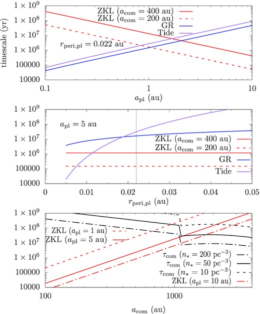
Time-scales of orbital precession caused by different mechanisms. The three panels show the time-scales for the planet’s orbital precession owing to the ZKL mechanism of a companion star in red (different line type for different apl and acom), the GR effect in red, tides in purple, and the lifetime of the companion star in black (different line type for different n*).
The value of bext is effectively the same as the largest possible bmax required by the combination of the highest scatterer mass, largest abin, and smallest vinf. We consider a binary scatterer with the two components each of 10 M⊙, abin = 1000 au, and vinf = 0.01 km s−1. Though vinf can be arbitrarily small, we note 0.01 km s−1 ≈ 0.01 pc Myr−1, and it takes such an encounter a few hundreds of Myr to traverse a typical open cluster of a few pc, so the chance of these slow encounters is small. With these extreme values, bext ∼ 8 pc and thus σext ∼ 2 × 10² pc2. The scattering frequency is consequently Γ = 200n* Myr−1 (where n* is in pc−3 and we have taken vinf = 1 km s−1), suggesting that the scatterings are extremely frequent. But a significant proportion of the encounters will not do anything appreciable either to the planetary system or to the scatterer (if binary), and do not need to be considered, because their b is larger than the respective bmax. Therefore, upon creating a scatterer with its time of encounter, mass orbit, b and vinf, if b > bmax, we simply omit this encounter and proceed to the next.
If the planetary system has an outer stellar companion, we will need to account for the evolution of the companion orbit during the encounters as well. Hence, in equation (2), now atot = acom + abin, the sum of the binary and the companion semimajor axes.
Those scattering events are simulated in a way similar to FEWBODY (Fregeau et al. 2004). On initiation, with the scatterer mass, vinf and b, we analytically move it to a distance such that the tidal perturbation on the star–planet/stellar binary system relative to their internal forcing is smaller than 10−4. During the scattering, we look for stable binary/triple systems recursively and the scattering is deemed finished if all triples are stable and/or the tidal perturbation on any binary by any other object is small again.
2.2 Simulation strategy
Tidal evolution has to do with the exchange of energy and angular momenta of the orbital motion and spins of the star/planet. While the tidal deformation in the planet is the main driver for the orbital circularization, that in the star is able to further modify the orbit afterwards. As the planet’s spin angular momentum is much less than that of its orbital motion, the orbital angular momentum is effectively conserved in the first stage.
In this work, we stop the propagation of a planetary system once the planet’s apocentre distance rapo, pl drops below 1 au in order to save computational time. We deem that beyond this point, the formation of an HJ is unlikely to be disrupted by further encounters or the small planet orbit makes it immune from further external perturbation and the formation of an HJ is impossible. Therefore, until this point, the planet’s orbit is still highly eccentric, and only the planetary tide is important in our simulation enabling a simple handling of the spins of the two objects. The planet, due to its small mass and physical radius, carries a much smaller spin angular momentum than that of the orbital motion and its spin is aligned and (pseudo-)synchronized with the orbital angular velocity at pericentre on a time-scale much shorter than that of orbital evolution (e.g. Hut 1981; Correia 2009). Hence, we simply let the spin of the planet be in that status in our simulation (e.g. Hamers & Tremaine 2017). Though during the ZKL cycles, the stellar spin may evolve in a very complicated manner (Storch, Anderson & Lai 2014), it is not expected to affect the orbital dynamics during the planet’s orbital shrinkage but may play a significant role latter on (e.g. Fabrycky & Tremaine 2007) beyond the scope of this work. We let the stellar spin be the current solar value, and align it with the initial orbital plane of the planet.
Both GR and tides are only effective when rperi, pl is small. In our code, the two are activated only if rperi, pl < 0.05 au (ten solar radii).
The code checks the planet’s orbital elements at the beginning and at the end of all scatterings and also routinely does so not during a scattering. If the planet’s apocentre distance drops below 1 au, and at the same time, the pericentre distance is below 0.02 au, we deem that an HJ forms.
Finally, the Bulirsch–Stoer integrator available in the mercury package (Chambers 1999) is adopted for propagating the state vectors of the objects using an error tolerance of 10−12, and collisions between the objects are also detected using the subroutines in mercury. The planetary system is followed for 1 Gyr, and the simulation is stopped if the planet becomes an HJ or does not orbit the original host anymore.
3 TIME-SCALES
Numerous authors have examined high-e migration in different context (e.g. Wu & Murray 2003; Fabrycky & Tremaine 2007, and see Naoz (2016) for a review). We would like to briefly review some of the relevant time-scales.
In the top panel of Fig. 1, we show the precession time-scales by the leading order ZKL effect in red, GR in blue, and tides in purple (the relevant expressions are taken from Naoz et al. 2013; Antognini 2015; Naoz 2016) as a function of apl fixing the planet pericentre rperi, pl = 0.022 au (where tidal effects becomes efficient in our model; see equation (3)). The companion orbit has been fixed at acom = 400 (solid line) or 200 au (dashed) and ecom = 0.7 (see Fig. 5 below for companion orbits from the simulations). Reading from the plot, the ZKL time-scale is inversely dependent on apl while those of GR and tide positively. For apl ≳ 1–2 au, the planet’s orbital precession is mainly driven by the companion star. Otherwise, those by GR and tides take over. Whereas the ZKL time-scale is insensitive to the epl, both GR and tides depend critically on it (or rperi, pl), and larger the rperi, pl, longer the latter two time-scales. This means for rperi, pl > 0.022 au, the ZKL effect prevails (at least for apl ≳ 1–2 au), and can excite epl to the point where tides are important.
In middle panel, these time-scales are shown as a function of rperi, pl (or equivalently epl), now fixing apl at 5 au. The time-scale of the ZKL mechanism does not depend on epl/rperi, pl and is shown as the red horizontal lines. Both GR and tides depend on rperi, pl and the latter more steeply. For rperi, pl ≳ 0.012 au, ZKL time-scale is the shortest among the three. This strengthens the above argument and means that for apl = 5 au, rperi, pl may be lowered to ∼0.012 au by the ZKL mechanism uninterruptedly.
We have shown in our model, a companion star at a few hundreds of au can, via the ZKL mechanism, pump the planet’s eccentricity high enough to trigger efficient tidal evolution, not interrupted by tides/GR or scattering stripping of the companion. But, we caution that the planet’s tidal orbital shrinkage and dynamical decoupling from the companion star may take many ZKL cycles (e.g. Wu & Murray 2003; Fabrycky & Tremaine 2007; Anderson, Storch & Lai 2016, and see Fig. 2 below) so the companion star has to survive much longer than the ZKL time-scale to this process. Therefore, the requirement that the ZKL time-scale is shorter than the companion lifetime is only necessary, but not sufficient for high-e migration. In the following, we present a few concrete examples.

Formation of an HJ via HJ_ZKL. The bottom panel shows the time evolution of the planet’s rperi, pl (red) and apl (blue) in the left y-axis and ipl, com (purple) in the right y; the top panel shows the companion’s rperi, com (red) and acom (blue) in left y-axis, and the planet’s hz (purple) in right y. The shaded regions represent ongoing stellar scattering; quantities related the companion’s orbit are not shown as it can be not well defined if the scattering is strong.
4 TEST SIMULATIONS
To validate our code, we first perform two sets of test simulations. In these simulations, the planet host is the Sun. In the first, the planet is much like our Jupiter with a circular orbit at 5 au from the central host. The normal tidal model (with Qtide, 0 = 107 and 5 × 10⁶ for the host star and the planet) is adopted. A total of 3000 runs are done. This set of simulations is referred to as our ‘Jupiter’ run. In the second set, the only difference is that the tidal quality factors are reduced by a factor of ten (with Qtide, 0 = 106 and 5 × 10⁵) and called ‘JupEnT’ (Jupiter enhanced tides). In both, the cluster property is n* = 50 pc−3 and binarity fbin = 0.5 (number of binary system divided by the sum of single and binary systems). The simulation parameters are listed in Table 1.
Initial set-up of the simulations. The first column is the simulation designation, the second the cluster stellar number density n*, the third the binarity fbin (the total number of binary star systems divided by the sum of the number of binary and single star systems), the fourth and the fifth the planet’s orbital semimajor axis apl and eccentricity epl, the sixth the tidal model, and the last the number of runs.
| Sim ID | n* (pc−3) | fbin | apl (au) | epl | Tidal model | |$\#_\mathrm{run}$| |
|---|---|---|---|---|---|---|
| Jupiter | 50 | 0.5 | 5 | 0 | normal | 3000 |
| JupEnT | 50 | 0.5 | 5 | 0 | enhanced | 3000 |
| Nominal | 50 | 0.5 | 1–10 | 0-0.95 | normal | 30000 |
| LowDen | 10 | 0.5 | 1–10 | 0-0.95 | normal | 3000 |
| HighDen | 200 | 0.5 | 1–10 | 0-0.95 | normal | 3000 |
| LowBin | 50 | 0.1 | 1–10 | 0-0.95 | normal | 3000 |
| HighBin | 50 | 0.9 | 1–10 | 0-0.95 | normal | 3000 |
4.1 Example planet evolution
Fig. 2 shows the formation of an example HJ from the Jupiter run. In the plot, the grey regions represent ongoing stellar scattering. Before 400 Myr, the system experiences only one scattering as without a companion, the system is only 5 au wide so a scatterer has to come with a very small impact parameter according to equation (2) to be potentially important but these are rare. This scattering event does not lead to appreciable changes in the planet’s rperi, pl (red, bottom panel, left ordinate) or apl (blue, bottom panel, left ordinate). Another scattering with a stellar binary occurs at 420 Myr, where the planetary system acquires a companion with pericentre distance rperi, com = 170 au (red, top panel, left ordinate) and acom = 850 au (blue, top panel, left ordinate); and the planet’s inclination with respect to the companion’s orbital plane is ipl, com = 57° (purple, bottom panel, right ordinate). Now ZKL cycles are activated in the planet’s orbit shown as the phase-correlated oscillations in rperi, pl and ipl, com. The purple line in the top panel shows the planet’s normalized vertical orbital angular momentum |$h_\mathrm{z}=\sqrt{1-e^2_\mathrm{pl}}\cos i_\mathrm{pl,com}$| relative to the companion’s orbital plane with the right y-axis, which is a conserved quantity in the lowest order ZKL theory. As expected, hz is quasi-constant, at least before the next stellar scattering.
The wide orbit of the companion means that more distant scatterings need to be taken into account, indicated by the increase in the number of the grey regions after the acquisition of the companion. During each of these (distant) scatterings, the planet’s orbit is not affected but the companion’s rperi, com and acom as well as its inclination ipl, com can be instantly altered. This also changes hz (because the reference plane changes) so after each scattering, the planet’s orbital elements evolve with a new pattern so rperi, pl and ipl, com reach different extrema.
Finally, during the scattering at 509 Myr, acom becomes 380 au, and ipl, com reaches almost 90°. Immediately after this encounter, rperi, pl is driven to <0.01 au. Then tidal effects quickly shrink the orbit to completely within 1 au during the first minimum of rperi, pl, so an HJ has formed and the simulation is stopped. This type of outcome is called HJ_ZKL (formation of HJ by a companion star). It is common (60 per cent of all the HJ_ZKL cases) for a companion star to experience stellar scatterings before it leads to the formation of an HJ.
Is the high-e migration process enhanced by these scatterings? To answer this question, we perform a simple test. For each system of the outcome HJ_ZKL, we have taken a snapshot of it the moment the system acquires the companion star that later leads to the HJ formation. From this snapshot, the system is propagated with the companion star in isolation without any scattering until 1 Gyr. It turns that an HJ only forms in 40 per cent of these simulations. This suggests that the scatterings between the companion star and other stars in the cluster have boosted the HJ formation.
Not all planets where ZKL cycles of appreciable amplitudes are enabled turn into HJs. For the vast majority of such planet orbits, the maximum epl is simply not large enough such that rperi, pl > 0.022 au and efficient tidal dissipation is never activated. And for another substantial fraction, the planet is driven into the central host by the companion – tides- and GR-induced orbital precession is outpaced by that of the ZKL effect so the latter goes untamed. The top panel of Fig. 3 shows such an example. At 494 Myr into the simulation, the planetary system obtains a companion star of acom = 700 au, ecom = 0.92, and ipl, com = 30°. Subsequently around 508 Myr, a scattering changes the companion orbit to acom = 720 au, ecom = 0.96, and ipl, com = 67°. Now the ZKL cycles are greatly amplified and after several cycles, noticeable higher-order effects manifest by driving down the extreme rperi, pl in each successive ZKL cycle (e.g. Naoz et al. 2011). Then at 501 Myr, when rperi, pl reaches 0.01 au, apl drops by ∼ 10 per cent by tides. During the subsequent dip of rperi, pl, the planet dives into the central host directly before tides are able to do anything. We note that the planet may be tidally disrupted by the star en route to a collision. But the tidal disruption limit for Jupiter around the Sun is about a few solar radii so we do not detect tidal disruption and generally call those collisions. The outcome of the collision with the central star as a result of the ZKL effect by the companion is referred to as COL_ZKL.
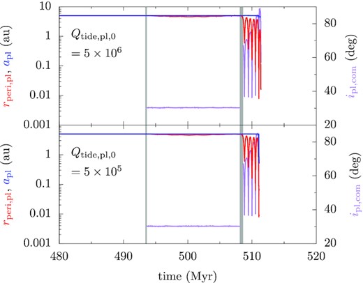
Time evolution of a planet that end up in the fates COL_ZKL and HJ_ZKL with different tidal Q. The left ordinate marks the planet’s rperi, pl (red) and apl (blue), and the right ordinate ipl, com (purple). The top panel shows the case of COL_ZKL, where the planet’s Qtide, pl, 0 = 5 × 10⁶, and the bottom panel of HJ_ZKL, where Qtide, pl, 0 = 5 × 10⁵; all the other parameters are the same in the two.
4.2 Statistics
We count the number of planets that have different fates and show their percentages in Table 2. The details of our simulations are presented in Section 2.2. The second column shows the percentage of the outcome HJ_ZKL, the third column HJ_SCAT (an HJ forms where the small rperi, pl is established during the scattering, but not forced by a bound companion star), the fourth column COL_ZKL, and the fifth column EJEC (Jupiter turns into a free floating planet without a host star).
Percentage of planets with different fates. The first column shows the ID of the simulation set; from the second to the fifth, those for HJ_ZKL (formation of HJ via the ZKL mechanism by a companion), HJ_SCAT (formation of HJ where the small pericentre distance is achieved directly during the scattering), COL_ZKL (collision forced by the ZKL mechanism by a companion), and EJEC (ejection) are shown. The errors are 1-σ dispersion from random resampling. The nominal set has 30 000 runs while the others have 3000 for each. In Section 5.4, the sum of HJ_ZKL and COL_ZKL will be also referred to as ZCT_ZKL.
| Sim ID | HJ_ZKL | HJ_SCAT | COL_ZKL | EJEC |
|---|---|---|---|---|
| Jupiter | |$2.43_{-0.26}^{+0.30}$| | 0 | |$5.80_{-0.41}^{+0.47}$| | |$23.6_{-0.7}^{+0.8}$| |
| JupEnT | |$4.27_{-0.40}^{+0.30}$| | |$0.0667_{-0.0667}^{+0.0333}$| | |$4.17_{-0.37}^{+0.33}$| | |$23.4_{-0.8}^{+0.7}$| |
| Nominal | |$2.43_{-0.09}^{+0.09}$| | |$0.127_{-0.017}^{+0.023}$| | |$3.64_{-0.11}^{+0.13}$| | |$20.1_{-0.2}^{+0.3}$| |
| LowDen | |$0.667_{-0.133}^{+0.133}$| | 0 | |$1.17_{-0.23}^{+0.17}$| | |$4.47_{-0.37}^{+0.37}$| |
| HighDen | |$4.74_{-0.46}^{+0.46}$| | |$0.0641_{-0.0641}^{0.0641}$| | |$7.37_{-0.64}^{+0.71}$| | |$52.4_{-1.2}^{+1.0}$| |
| LowBin | |$0.667_{-0.133}^{+0.133}$| | 0 | |$0.967_{-0.167}^{+0.200}$| | |$8.87_{-0.50}^{+0.43}$| |
| HighBin | |$3.77_{-0.37}^{+0.34}$| | |$0.100_{-0.067}^{+0.039}$| | |$6.23_{-0.37}^{+0.50}$| | |$29.6_{-0.8}^{+0.7}$| |
Table 2 shows that about 24 per cent of the planets are ejected for both the Jupiter and the JupEnT runs. This can be compared to the simple predictions from equation (1). That equation when integrated over time, prescribes the chance that an event happens for a planetary system knowing the respective cross section σ. A number of authors have estimated that for EJEC under different assumptions (e.g. Laughlin & Adams 1998; Adams et al. 2006; Li & Adams 2015; Wang, Perna & Leigh 2020a); here we take the value from Li et al. (2020b), where the set-up was the most similar to this work. From there, σEJEC = 9.7 × 10⁴ au2 implies a percentage of 12 per cent for EJEC in 1 Gyr for Jupiter’s ejection. So the two differ by a factor of two. Li et al. (2020b) also measured the σ for the Sun–Jupiter pair to acquire a companion star, and the inference was that almost all are expected to have a companion within 1 Gyr. Here, we find that 46 per cent of the planetary systems in the Jupiter run obtain at least companion at some point in the simulation. Therefore, the percentages in this work agree with the expectations reasonably well.
Considering the HJs in the Jupiter run, the percentage of HJ_ZKL is 2.4 per cent and that of HJ_SCAT is a hundred times smaller. So the formation of HJ as a direct result of a scattering is extremely rare (Hamers & Tremaine 2017). Compared to HJ_ZKL, a significantly larger proportion, 5.8 per cent end up as COL_ZKL, meaning that in many cases, the ZKL cycle is not quenched by GR or tides. The temporal evolution of the percentages will be deferred to Section 5.4, where we derive their time dependence.
In our treatment of tides, equation (3) prescribes how Qtide varies depending on the planet orbit (Beauge & Nesvorny 2012), and is a fit to the model of Ivanov & Papaloizou (2011). Taking our nominal simulation as an example, the minimum possible planetary Qtide corresponding to the most efficient tidal damping is achieved when the planet is just touching the surface of the central host, and is about 2000 for apl = 5 au. However, works looking into different modes have suggested that for extremely eccentric orbits, the equivalent Q can be much smaller, possibly reaching a few tens or even a few (e.g. Wu 2018; Yu, Weinberg & Arras 2022). With a more efficient tidal model, planets of the fate COL_ZKL may end up HJ_ZKL.
Fig. 3 shows such an example. The initial conditions of the planetary system as well as the sequences of the stellar scatterings are exactly the same for the two panels. As we discussed earlier, when Qtide, pl, 0 = 5 × 10⁶ (top panel), tidal dissipation is not fast enough and the ZKL effect goes unsuppressed and forces the planet onto the star (COL_ZKL). When Qtide, pl, 0 = 5 × 10⁵ (bottom panel), tides efficiently shrinks the planet’s orbit, detaches it from the companion star, and hence stops further eccentricity excitation by the ZKL mechanism and an HJ forms (HJ_ZKL).
As Table 2 shows, for the JupEnT run, the percentage for HJ_ZKL and CKL_ZKL are almost the same, both about 4.2 per cent, so the creation of HJ_ZKL is boosted by 70 per cent. But the sum of HJ_ZKL and CKL_ZKL is 8.3 per cent, which is in excellent agreement with the Jupiter run, a phenomenon seen also in Petrovich (2015), Anderson et al. (2016), Muñoz, Lai & Liu (2016). In the JupEnT set, the percentage of HJ_SCAT and EJEC are not affected by enhanced tides, both only related to the scattering process.
Additionally, about 1.5 per cent of the planets collide with their host star during the scattering, and 1.2 per cent acquire orbits bound to the scatterer. We have omitted discussion on these two states as they will not affect the creation of HJs. But we note that both percentages are roughly a tenth of that of EJEC, consistent with the ratios of their respective cross sections as derived in Li et al. (2020b).
5 POPULATION SYNTHESIS
In the previous section, we have shown with concrete examples that HJs may form via high-e migration initiated by a companion star that the planetary host star acquires during a binary–single scattering in a stellar cluster. In this section, we perform sets of population synthesis simulations, and explore the dependence of the efficiency of this mechanism on the properties of the cluster and the planetary system.
5.1 Simulation parameters
We fix the central host to be the Sun and the planet’s physical parameters to be those of Jupiter. For all the runs, the tidal model has been the normal one (3), and no enhancement is effected. The planet’s orbital distribution as we detail below is also the same for all following runs.
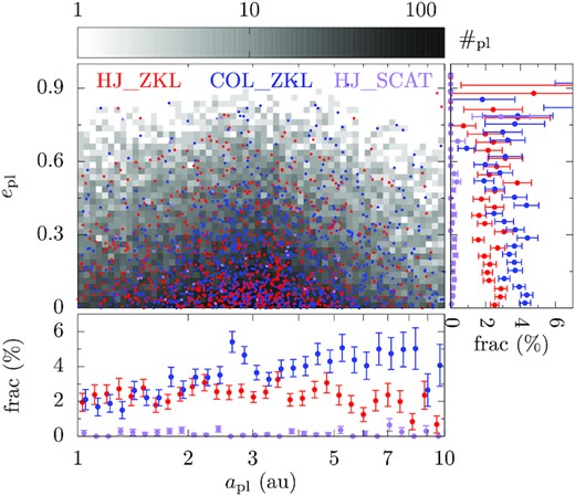
The initial orbital distribution of the planets and their fates for the Nominal set-up. The grey histogram in the big panel shows the planets’ distribution in the apl − epl plane, darker colours meaning more planets, as shown in the colour bar above. In that panel, the scattered points show those that have the fates HJ_ZKL (red), COL_ZKL (blue), and HJ_SCAT (purple). The bottom and the right-hand panels show the percentage of planets with those fates as a function of the initial orbit; the error bars are 1-σ dispersion from a bootstrapping process; the points are slights shifted for better presentation.
Our eccentricity distribution follows a Beta distribution as proposed by (Kipping 2013) for radial velocity planets.1 An upper limit of epl = 0.95 is set, as this coincides roughly with the highest observed eccentricity among the radial velocity planets (e.g. HD 20782 b, though in a very wide binary system; see Jones et al. 2006), and also insures that initial tidal effect is negligible even for apl = 1 au.
In one set of the runs, the cluster parameters are the same as the Jupiter run, i.e. n* = 50 pc−3 and fbin = 0.5. This forms our main simulation set and is called the ‘Nominal’ set. A total of 30 000 runs are done for this set.
Four additional sets of simulations with different cluster properties are performed. In the sets ‘LowDen’and ‘HighDen’, n* = 10 and 200 pc−3, respectively, both with fbin = 0.5. And in the sets ‘LowBin’ and ‘HighBin’, fbin = 0.1 and 0.9, respectively, both with n* = 50. For those, 3000 runs are done for each. These parameters are listed in Table 1.
5.2 Results of the Nominal simulation set
We first analyse the results of the Nominal set. Table 2 shows that the percentage of HJ_ZKL is 2.4 per cent, that of HJ_SCAT 0.13, 3.6 per cent for COL_ZKL, and 20 per cent for EJEC. In comparison to the Jupiter run, it seems that the change is mild – the creation of HJ_ZKL has the same efficiency and that of EJEC decreases by less than 20 per cent; HJ_SCAT is enhanced by a factor of a few, but its contribution to the formation of HJs is anyway less efficient by a factor of at least 20 compared to HJ_ZKL. For COL_ZKL, there is a 40 per cent boost (at ∼5 − σ level) in the Nominal run compared to the Jupiter run.
How does the planet’s initial orbit affect its fate? The large panel of Fig. 4 displays as scattered points the initial orbital distribution of the planets in the final states HJ_ZKL (red), COL_ZKL (blue), and HJ_SCAT (purple). The bottom and the right-hand panels of that figure present the percentage of planets with the three fates as a function of apl and epl.
The figure suggests that HJ_ZKL does not depend on the initial epl, and seems to show a weak negative dependence on apl (e.g. Muñoz et al. 2016). The planet’s apl affects the planet’s evolution in many aspects. Fig. 1 shows that for a fixed acom, a larger apl means a smaller ZKL time-scale, facilitating HJ_ZKL. But this could turn out to be an adverse effect as the ZKL effect could go untamed (by GR/tides) so that the planet collides with the central host. On the other hand, efficient tidal dissipation has to be activated so the planet’s orbit can be shrunk. From our tidal model, this means |$e_\mathrm{pl} > 1-0.022\, \mathrm{au}/a_\mathrm{pl}$|. Apparently, the larger the apl the higher the epl is needed; this works against HJ_ZKL for a larger apl. Moreover, embedded in a cluster, the constant stellar scatterings may alter the companion star’s orbit and, therefore, interrupt the ZKL cycle. Overall, HJ_ZKL shows a weak negative dependence on apl while for COL_ZKL, a clearer positive dependence is seen.
Similarly, the effect of the initial epl on HJ_ZKL is weak. This is seemingly counter-intuitive since a larger initial epl reduces the requirement on ipl, com to excite epl to the same level (e.g. Li et al. 2014). Take apl = 5 au for example, epl has to reach 0.996 to enable tidal dissipation (so rperi, pl = 0.022 au). Using the leading order ZKL theory, we have performed a simple Monte Carlo simulation fixing the initial epl and randomly drawn ipl, com, and phase angles and the fraction of orbits that can achieve a maximum epl of at least 0.996 is calculated. We find that this fraction depends on epl very mildly and an increase of the initial epl from ∼0 to ∼0.9 only boosts the fraction by 100 per cent. But planets with initial epl ≳ 0.9 are rare in our simulations. This seems at odds with Mustill et al. (2022a). In explaining the observed high eccentricity of HR5183b, Mustill et al. (2022a) found that an initial epl (which might be caused by planet–planet scattering) would enhance the chance that a companion excites epl to the observed value. In that work, the authors were examining the fraction of time that epl is higher than a certain value whereas here it is the maximum epl ever attained that matters.
We would like to assess what kind of scattering binaries help create HJ_ZKL, and how the properties of the companions are distributed for these systems. But this may not be as straightforward as it may seem. As Fig. 2 shows, the orbit of the planetary system’s companion is subject to further alteration due to stellar scattering. In that example, the companion star has remained bound to the planetary system so the binary scatter that this companion is in originally is the one that contribute directly to HJ_ZKL. But it can be more complicated in that we have registered in our simulations cases, where the planetary system obtains a companion star after scattering with a binary and an HJ does not form; after interactions with other scatterers (single or binary), the original companion swaps with another star, and this companion triggers the process of HJ_ZKL. In this latter case, if the companion at the time of the formation of the HJ comes from a binary scatterer, we record the orbit of that binary; if not, we trace back to see if the predecessor of the companion is from a binary and so on and so forth. The top left-hand panel of Fig. 5 shows the semimajor axis of the scattering binary abin as a function of the mass mcom of the companion of the planetary system. The top right and the bottom panels show the histogram of abin and mcom, respectively. The mass mcom covers the full range of our initial mass function with a median of 0.42 M⊙ while abin is broadly distributed from tens to hundreds of au with a median of 110 au. The middle-left-hand panel of the figure shows the companion’s acom as a function of mcom, and the middle right is the histogram of acom. Compared to the broad distribution abin, acom is more centred around the median 220 au.
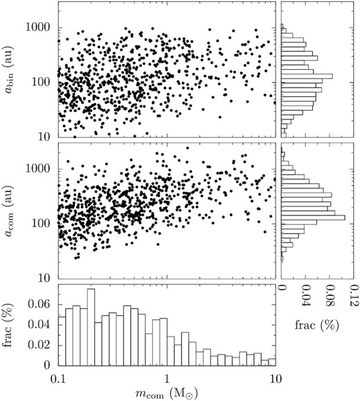
The distribution of the scattering binary’s abin leading to the outcome of HJ_ZKL, and the planetary system’s companion’s acom as a function of the companion mass mcom in the nominal set. From top to bottom, the three histograms show the distribution of abin, acom, and mcom.
Many workers have carried out population synthesis studies on HJ formation via the ZKL mechanism (Naoz, Farr & Rasio 2012; Petrovich 2015; Anderson et al. 2016; Muñoz et al. 2016; Vick, Lai & Anderson 2019). Due to the inherently different assumptions (like the usage of secular/full equations of motion, the tidal model, and the cluster environment), our HJ formation rate HJ_ZKL cannot be compared directly with theirs. But many common characteristics are observed: e.g. the general HJ_ZKL rate of a few per cent and the invariability of the sum of the rates of COL_ZKL, and HJ_ZKL under different tidal efficiencies (see Table 2 and Petrovich 2015; Anderson et al. 2016; Muñoz et al. 2016). And the cluster environment also introduces new features. For instance, the preferred companion separation for HJ_ZKL here under stellar scatterings (a few hundreds of au) is appreciably smaller than if the systems are in isolation (wider than several hundreds of au Naoz et al. 2012; Petrovich 2015) as a result of the disruption of the companion orbit.
5.3 Results of the other runs
The percentages of different fates for the other simulation sets are presented in Table 2.
First, what role does the stellar number density n* play? By comparing the sets LowDen and HighDen with the Nominal simulation, we observe that decreasing/increasing n* has the effect of counteracting/boosting the percentage of HJ_ZKL. Obviously, a lower/higher n* implies a lower/higher scattering rate, which diminishes/enhances the chance that a planetary system acquires a companion star and, therefore, the probability of HJ_ZKL. Also, a lower/higher n* implies a longer/shorter lifetime of the so-acquired companion star, allowing the ZKL effect more/less time to operate. According to Fig. 1, even for the HighDen run, for any acom ≲ 1000 au, the ZKL time-scale is much shorter than the companion lifetime. Therefore, the constraint from the companion star’s survivability is weak (but higher order effects, not reflected in that figure, can operate on much longer time-scales; see e.g. Ford et al. 2000; Naoz et al. 2011; Antognini 2015) and as a consequence, for the parameter range considered here, a higher n* means a higher percentage of HJ_ZKL. But, the dependence may not be linear. Comparing the Nominal with the HighDen run, an increase of n* from 50 to 200 pc−3 only increases the percentage of HJ_ZKL by a factor of two, the main reason being that 1.5 times more planets are ejected in the denser environment so the reservoir for HJ_ZKL is significantly smaller. A comparison between the Nominal and the LowDen runs shows that decreasing n* by 80 per cent leads to a drop in the percentage of HJ_ZKL by more than 70 per cent, so the linearity towards smaller n* is more pronounced.
Much like the influence of n*, fbin affects a planetary system in two ways: increasing the prospect of the acquisition of a companion star and decreasing the lifetime of the companion. It turns out that a higher fbin (HighBin) gives rise to a higher percentage of HJ_ZKL and vice versa (LowBin). We note that in the LowBin run, the effective density for binaries (nbin = n*fbin) is 50 pc−3 × 0.1 = 5 pc−3 coincident with that in the LowDen run 10 pc−3 × 0.5 = 5 pc−3, and the percentages of HJ_ZKL are in excellent agreement in the two sets of simulations. This suggests that (when EJEC is not overwhelming) the percentage of HJ_ZKL depends on the binary spatial density nbin of the cluster only.
Then, not surprisingly, in all simulations, the percentage of HJ_SCAT is smaller than that of HJ_ZKL by at least an order of magnitude, so we omit discussion on the former. And for all these simulation sets, the ratio of the percentage of COL_ZKL and HJ_ZKL is about constant ∼1.5, consistent with the expectation both are results of the ZKL mechanism, and depend on the cluster property in similar ways. Therefore, we may broadly refer to both COL_ZKL and HJ_ZKL as ACT_ZKL, meaning that extreme ZKL cycles are activated, where the planet either turns into an HJ or plummet into the central host, i.e. ACT_ZKL = COL_ZKL + HJ_ZKL.
5.4 Empirical dependences on cluster parameters
In general, the rate that an event happens can be estimated with equation (1) by plugging in the appropriate σ. In calibrating σ, previous works have often separated the effects of binary and single stars (Adams et al. 2006; Li & Adams 2015; Li et al. 2020b). Here, we follow the same approach.
In our scenario, ACT_ZKL is only affected by the binaries and single stars cannot contribute. So the rate of ACT_ZKL can be approximated by |$A_\mathrm{z} {n_\mathrm{bin}\over 1\, \mathrm{pc}^{-3}}$|, where AZ is a constant to be determined.
The top panel of Fig. 6 shows the time evolution of the percentage of ACT_ZKL for all the five population synthesis simulation sets. And we have fitted those curves using equation (11) above, and the fitting parameters are Az = (3.0 ± 0.05) × 10−6, Ar = (1.6 ± 0.2 × 10⁻⁵, Br = (6.3 ± 1) × 10−6. The result from the fit is also presented. The agreement is fairly good and the largest deviation is within two sigma. It seems that while the percentage of ACT_ZKL for the HighDen set is plateauing toward the end of the simulation, those for the other sets are still steadily increasing.
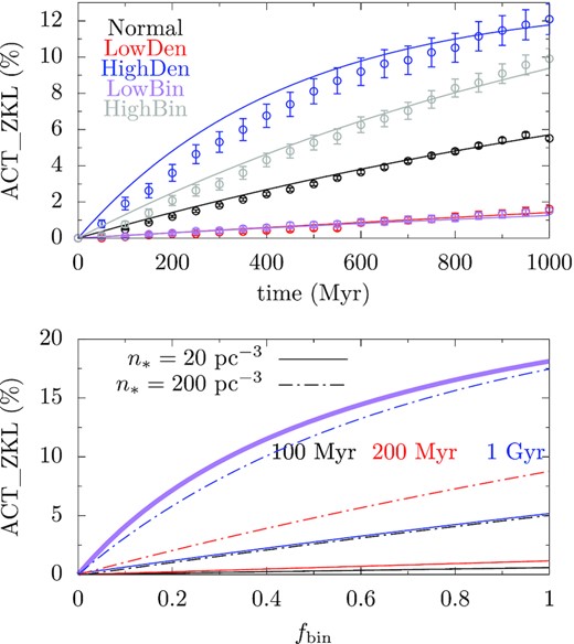
Percentage of planets with the outcome ACT_ZKL, the sum of HJ_ZKL and COL_ZKL. The top panel shows the time evolution of ACT_ZKL from different runs (points), and the respective fits (line) in different colours. The bottom panel shows the percentage of ACT_ZKL as a function of fbin for n* = 20 (solid line) and 200 pc−3 (dash–dotted line) at 100 Myr (black), 200 Myr (red), and 1 Gyr (blue). The thick purple line is the upper limit of the percentage for a given fbin.
The density n* prescribes how quickly the percentage of ACT_ZKL approaches that limiting value. In the bottom panel of Fig. 6, we plot the percentage of ACT_ZKL as a function of fbin at 100 Myr (black), 200 Myr (red), and 1 Gyr (blue) for n* = 20 pc−3 (solid line) and 200 −3 (dash–dotted line). For the lower density, the percentages at all times are quasi-linearly dependent on fbin, but for the higher density, the percentage of ACT_ZKL saturates toward the upper limit, implying that the limit can be reached within a few Gyr for n* of a few hundred pc−3.
Finally, we note that a fraction of those ACT_ZKL will be indeed HJ_ZKL while the others will be COL_ZKL. The exact division depends on the details of the tidal interaction; see the simulation sets Jupiter and JupEnT in Section 4.2 for a discussion. But the chances for ACT_ZKL and HJ_ZKL are comparable.
6 DISCUSSION
6.1 Observational implications
As reviewed in the introduction section already, the observations of planets in clusters have been sparse with only a few HJs detected so far. Here, we only discuss those found in dedicated surveys but not otherwise (e.g. Obermeier et al. 2016; Ciardi et al. 2017; Rizzuto et al. 2018; Livingston et al. 2019).
In total, 3 HJs have been found around 160 stars in Praesepe (NGC 2632) and Hyades (Paulson et al. 2004; Quinn et al. 2012, 2014) so the HJ occurrence rate is 2 per cent. Both clusters are ∼600 Myr old and metal rich. After correcting for the solar metallicity, a rate of 1 per cent was derived (Quinn et al. 2014), consistent with that of the field (Wright et al. 2012).
Brucalassi et al. (2016) surveyed 66 stars in M67 (NGC 6282) which is of solar metallicity and age. Three HJs were found so the ccurrence rate is 4.5 per cent; removing the 12 stars that are in binaries, the HJ ccurrence rate around single stars was 5.6 per cent. These numbers are much higher than that of the field (e.g. Wright et al. 2012). M67 has a high |$f_\mathrm{bin}\sim 30\!-\!40\ \hbox{per cent}$| on average, but could be as high as 70 per cent near the centre (Davenport & Sandquist 2010; Geller et al. 2021). Being among the oldest open clusters, M67 is highly evolved. From N-body simulations producing predictions consistent with the observations, the cluster probably through its lifetime has lost the majority of its total mass, and n* at the core has remained largely around 100 pc−3, and fbin has not evolved significantly either (Hurley et al. 2005; Hurley, Aarseth & Shara 2007). Combined this means that at the core (where solar mass stars sink to), nbin is perhaps several tens to a hundred pc−3 within the optimal range for the HJ_ZKL production from the bottom panel of Fig. 6. If like the field, the primordial giant planet occurrence rate is 10–20 per cent within a few au (e.g. Cumming et al. 2008) at the core of M67, our mechanism would predict an HJ occurrence rate of 1–2 per cent. But, we note these inferences are to be treated with caution; see Section 6.3 for a brief discussion.
6.2 Comparison with other mechanisms
Several works have been dedicated to the formation of HJs in star clusters. Shara, Hurley & Mardling (2016) used full fledged N-body cluster simulations to address this issue, propagating the evolution of massive ∼2 × 10⁴-member clusters with a binarity of 0.1 to a few Gyr. Their derived HJ formation rate is 0.4 per cent per star or 0.2 per cent per planet, and suggested that maybe tripling the binarity could increase the formation rate by 200 per cent. Hamers & Tremaine (2017) examined how (multiple) stellar scattering helps create HJs via high-e migration in globular clusters. Unlike in open clusters, in these densely-populated environment, ejection is likely to remove most of the planets (e.g. Davies & Sigurdsson 2001). After a careful search, Hamers & Tremaine (2017) found that for an initial semimajor axis of a few au, the favourable stellar density for making HJs is a few times 104 pc−3. Wang et al. (2020b) investigated the long-term evolution of a two-planet system after stellar fly-bys, concluding that higher-e migration could be triggered by interplanetary ZKL mechanism and/or pure scattering, the former more efficient when the two orbits are wide apart. Rodet et al. (2021) looked at a similar two-object scenario but concentrated on the case of wide-separation orbits. More recently, Wang et al. (2022) found that a multiplanet system may gain enough angular momentum deficit such that the system may become unstable afterwards and one of the planets might become an HJ.
Due to the different assumptions, it is impossible to make a full comparison between these works and ours. We just make some comments below.
Hamers & Tremaine (2017) considered a single-planet system and omitted binary stars, so therein, the planet’s small pericentre distance can only be achieved during the scattering, in some sense close to our case HJ_SCAT. From our simulations, the rate is for HJ_SCAT |${\lesssim}0.1\ \hbox{per cent}$| for a typical open cluster set-up. This implies for single-planet systems in open clusters, our HJ_ZKL mechanism is the most efficient.
Shara et al. (2016), Wang et al. (2020b, 2022), Rodet et al. (2021) have all considered multiplanet systems. In order for instability or ZKL effects to occur within the planetary system, significant orbital angular momentum must be extracted from the outermost object during the scattering, and the closest distance between the scatter and the planetary system must be comparable to the size of the latter. Therefore, a ‘close scattering’ for the planetary system is needed, and wider the planetary system more efficient their models work. In contrast, in our model, the scattering occurs between a planetary and a stellar binary, and the former, as a whole, exchanges with a component of the latter. Hence, the closest distance during the scattering only needs to be comparable to size of the stellar binary, which is often much larger than that of the planetary system. In this sense, a ‘close scattering’ for the planetary system is not needed and the system never experiences instantaneous orbital alterations during the scattering. Not relying on a wide planetary system, our mechanism probably works better for compact systems.
6.3 Caveats
In this work, we have tracked the evolution of a one-planet system in an open cluster, simulating its scattering with single and binary stars using a simple Monte Carlo approach. In order to study the effect of our proposed formation mechanism for HJs, several potentially important factors have been omitted.
Open clusters, as the name suggests, are slowly losing their mass owning to member star ejection, and stellar evolution (Lamers & Gieles 2006). In the meantime, cluster properties, like fbin, and n*, may also evolve considerably over many-Myr time-scales (e.g. Kroupa 1995). Moreover, the parent cluster may be born with substructures, where these diffuse on many-Myr time-scales (e.g. Goodwin & Whitworth 2004; Parker & Meyer 2012; Parker & Quanz 2012). Section 5.4 suggests that the rate of ACT_ZKL asymptotically approaches a value determined by the cluster’s fbin on a time-scale typically of 1 Gyr. Therefore, the cluster’s parameters used in this work are Gyr-averaged values.
The binary evolution has also been ignored. Wider binaries may be subject to disruption owing to stellar scattering (e.g. Kroupa 1995; Parker et al. 2009). Fig. 1 shows that those wider than a few hundreds of au would have been disrupted at a few hundreds of Myr so they cannot contribute to the formation of HJs at a later time. However, Fig. 5 shows that about half of the binary scatterers that lead to the formation of HJs via HJ_ZKL have abin < 100 au, and are largely immune from break-up. So the disruption of wide binaries in the cluster will potentially halve the HJ formation percentage we predict.
Then, the stellar evolution is also omitted. In a Gyr, a ∼2 M⊙ star will evolve off the main sequence, shedding a large fraction of the initial mass (e.g. Hurley, Pols & Tout 2000). If in a binary, this may cause the binary orbit to expand or even disrupt the binary totally (e.g. Veras et al. 2011). Fig. 5 shows that most of the companion stars (78 per cent) that contribute to HJ_ZKL are below 1 M⊙, and only 11 per cent of the companions are above 2 M⊙. All such binaries are wide so when the massive companion is evolved, the Roche lobe will not be filled and the two stellar components evolve in isolation. Then as the stellar masses is being lost, the companion’s orbit expands, making the ZKL time-scale longer, and itself vulnerable to scattering disruption and the outcome of HJ_ZKL unlikely.2 Removing those stars, the percentage of HJ_ZKL would drop by a few tens of per cent.
Studies of planets in clusters are limited by the relatively small number of stars in clusters compared to the field. Recently, Winter et al. (2020) calculated the phase-space density for field stars using the full stellar kinematic information (position and velocity), and found the HJ occurrence rate was higher for stars in overdensities (which arise very much as a result of small relative velocities but not spacial proximity). Further analyses suggested that the multiplicity of a planetary system (Longmore, Chevance & Diederik Kruijssen 2021), the architecture of multiplanet systems (Chevance, Diederik Kruijssen & Longmore 2021), and the occurrence rates of some types of planets (Dai et al. 2021) also have to do with the overdensities. If high-phase-space density now were to arise from a high-density birth environment, this would be a powerful tool to study the effects of birth environments on planetary system formation and early evolution. However, the statistical significance of these findings is questionable (Adibekyan et al. 2021). And it has been found that the stellar overdensities reflect the galactic kinematic/dynamical evolution (Kruijssen et al. 2021; Mustill, Lambrechts & Davies 2022b), and are not necessarily relics of a clustered star formation. Therefore, we shy away from discussing the implications of these results on our result.
Finally, we have only examined a lone planet around a solar mass star. Statistically, how a multiplanet system evolves under stellar scattering depends on the architecture of the system, and instant instability, delayed instability may result (e.g. Malmberg et al. 2011; Li et al. 2019, 2020a; Wang et al. 2022). If the system acquires a companion star, ZKL cycles/instability may be initiated or not also depending on the planets’ configuration (e.g. Innanen et al. 1997; Malmberg et al. 2007a; Marzari, Nagasawa & Goździewski 2022). To present a thorough discussion on this is beyond the scope of this work.
7 CONCLUSIONS
We have proposed a formation channel for HJs in open star clusters: a planetary system, through binary–single interactions, acquires a companion star, which then excite the planet’s orbit through ZKL mechanism, activating high-eccentricity migration, and giving rise to the creation of an HJ. Using Monte Carlo simulations, we have modelled how a solar mass star hosting a lone gas giant planet scatters with binary, and single stars successively in an open cluster tracking the evolution of the planet under Newtonian gravity, GR, and tides. Our main findings are as follows.
If a solar mass star hosts a giant planet at a few au, and acquires a companion star a few hundreds of au distant that companion is able to excite the planet’s orbit through ZKL mechanism, before it is stripped by stellar scattering in the cluster.
As a consequence, the planet’s pericentre distance rperi, pl may reach a few solar radii. If so, the planet’s orbit can be shrunk by tidal dissipation in a few Myr and an HJ results.
In our nominal cluster with n* = 50 pc−3 and fbin = 0.5, ∼2 per cent of single gas giants orbiting a solar mass star between 1 and 10 au will become an HJ through the above channel in a Gyr.
In the meantime, ∼4 per cent of the planets collide with or are tidally disrupted by the host star because of the large-amplitude ZKL oscillations forced by the companion star.
And about 20 per cent of the planets are ejected from their host star owing to stellar scattering.
A far smaller percentage |${\lesssim}0.1\ \hbox{per cent}$| of the planets can acquire a small pericentre distance directly during stellar scattering, and become HJs without the need of a companion star.
The total percentage of the formation of HJ and collision/tidal disruption depends on the cluster properties. The cluster fbin sets an upper limit that will be reached given enough time (10 per cent at fbin = 0.3 and 18 per cent at fbin = 1). And how quickly the above limit is reached depends linearly on n*: a few Gyr for n* of a few hundred pc−3.
Adopting a more efficient tidal model turns a fraction of the planets with the outcome collision into HJs. In general, the likelihoods of the formation of HJ and collision are comparable.
ACKNOWLEDGEMENTS
The authors are grateful to the anonymous referee for the comments and suggestions that help improve the manuscript. The authors acknowledge financial support from the National Natural Science Foundation of China (grants 12103007 and 12073019), the Swedish Research Council (grant 2017-04945), the Swedish National Space Agency (grant 120/19C), and the Fundamental Research Funds for the Central Universities (grant 2021NTST08). This work has made use of the HPC facilities at Beijing Normal University.
DATA AVAILABILITY
The data underlying this paper will be shared on reasonable request to the corresponding author.
Footnotes
Random number generators by Richard Chandler and Paul Northrop have been used https://www.ucl.ac.uk/~ucakarc/work/randgen.html.
