


ABSTRACT
The masses of galaxy clusters can be measured using data obtained exclusively from wide photometric surveys in one of two ways: directly from the amplitude of the weak lensing signal or, indirectly, through the use of scaling relations calibrated using binned lensing measurements. In this paper, we build on a recently proposed idea and implement an alternative method based on the radial profile of the satellite distribution. This technique relies on splashback, a feature associated with the apocentre of recently accreted galaxies that offers a clear window into the phase-space structure of clusters without the use of velocity information. We carry out this dynamical measurement using the stacked satellite distribution around a sample of luminous red galaxies in the fourth data release of the Kilo-Degree Survey and validate our results using abundance-matching and lensing masses. To illustrate the power of this measurement, we combine dynamical and lensing mass estimates to robustly constrain scalar–tensor theories of gravity at cluster scales. Our results exclude departures from General Relativity of the order of unity. We conclude the paper by discussing the implications for future data sets. Because splashback mass measurements scale only with the survey volume, stage-IV photometric surveys are well-positioned to use splashback to provide high-redshift cluster masses.
1 INTRODUCTION
The majority of ordinary matter, a.k.a. baryonic matter, is thought to be trapped inside the potential wells of the large-scale structure of the Universe. The main constituent of this invisible scaffolding is dark matter, and its fully collapsed overdensities, known as haloes, contain most of the mass in the Universe. These structures are not isolated, and the process of structure formation is known to be hierarchical (Press & Schechter 1974). In simple terms, this means that smaller haloes become subhaloes after they are accreted on to larger structures. Unsurprisingly, baryonic matter also follows this process, resulting in today’s clusters of galaxies. Due to their joint evolution, a tight relationship exists between the luminosity of a galaxy and the mass of the dark matter halo it inhabits. These galaxy clusters are associated with the largest haloes in the Universe and they are still accreting matter from the surrounding environment, i.e. they are not fully virialized yet.
Galaxies can be divided into two populations: red and blue (Strateva et al. 2001). Whereas red galaxies derive their colour from their aging stellar population, blue galaxies display active star formation, and young stars dominate their light. The exact mechanism behind quenching, i.e. the transition from star-forming to ‘red and dead’, is still not fully understood (see e.g. Schaye et al. 2010; Trayford et al. 2015), but it is known to be connected to both baryonic feedback (see e.g. Somerville et al. 2008; Schaye et al. 2010) and interactions inside the dense cluster environment (see e.g. Larson, Tinsley & Caldwell 1980; Moore et al. 1996; van den Bosch et al. 2008). An important consequence of this environmental dependence is the formation of a red sequence, i.e. a close relationship between the colour and magnitude of red galaxies in clusters. By calibrating this red sequence as a function of redshift, it is possible to identify clusters in photometric surveys, even in the absence of precise spectroscopic redshifts (Gladders & Yee 2000).
In recent years, splashback has been recognized as a feature located at the edge of galaxy clusters. The radius of this boundary, rsp, is close to the apocentre of recently accreted material (see e.g. Adhikari, Dalal & Chamberlain 2014; Diemer 2017; Diemer et al. 2017) and it is associated with a sudden drop in matter density. This is because it naturally separates the single and multistream regions of galaxy clusters: orbiting material piles up inside this radius, while collapsing material located outside it is about to enter the cluster for the first time.
In simulations and observations, the distribution of red galaxies and dark matter in the correlated structure surrounding clusters seem to trace this feature in the same fashion (Contigiani, Bahé & Hoekstra 2021; O’Neil et al. 2021), with a possible dependence on secondary galaxy properties (Shin et al. 2021; O’Neil et al. 2022). For the sake of clarity, we point out that both the literature and this paper refer to correlated substructures as satellites, even if their population is not entirely composed of objects gravitationally bound to the cluster.
In the wider context of galaxy evolution models, the mechanism behind this feature has been known under the name backsplash for almost two decades and has been previously explored both in observations and simulations (Gill, Knebe & Gibson 2005; Mahajan, Mamon & Raychaudhury 2011). Compared to these efforts, however, the recent interest in this feature is guided by theoretical and observational implications for the study of the large-scale structure of the Universe.
Observationally, one of the most noteworthy applications of the splashback feature is the study of quenching through the measurement of the spatial distribution of galaxy populations with different colours (Adhikari et al. 2021). While notable, this was not the earliest result from the literature, and many other measurements preceded it. Published works can be divided into three groups: those based on targeted weak lensing observations of X-ray selected clusters (Umetsu & Diemer 2017; Contigiani, Hoekstra & Bahé 2019b), those based on the lensing signal and satellite distributions around SZ-selected clusters (see e.g. Shin et al. 2019), and those based on samples constructed with the help of cluster-finding algorithms applied to photometric surveys (see e.g. More et al. 2016; Chang et al. 2018). However, we note that in the case of the last group, the results are difficult to interpret because the splashback signal correlates with the parameters of the cluster detection method (Busch & White 2017).
In this work, we implement an application of this feature based on Contigiani et al. (2021). The location of the splashback radius is connected to halo mass, and its measurement from the distribution of cluster members can therefore lead us to a mass estimate. Because this distribution can be measured without spectroscopy, this means that we can extract a dynamical mass purely from photometric data. To avoid the issues related to cluster-finding algorithms explained above, we studied the average distribution of faint galaxies around luminous red galaxies (LRGs) instead of the targets identified through overdensities of red galaxies. If we consider only passive evolution, the observed magnitude of the LRGs can be corrected to construct a sample with constant comoving density (Rozo et al. 2016; Vakili et al. 2019), and, by selecting the brightest among them, we expect to identify the central galaxies of groups and clusters.
We present our analysis in Section 3 and produce two estimates of the masses of the haloes hosting the LRGs in Section 4. The first is based on the splashback feature measured in the distribution of faint galaxies, while the second is based on the amplitude of weak lensing measurements. After comparing these results with an alternative method in Section 5, we discuss our measurements in the context of modified models of gravity. We conclude by pointing out that, while we limit ourselves to redshifts z < 0.55 here, the sample constructed in this manner has implications for the higher redshift range probed by future stage-IV photometric surveys (Albrecht et al. 2006) such as Euclid (Laureijs et al. 2011) and the Legacy Survey of Space and Time (LSST; LSST Science Collaboration 2009). Section 5.2 discusses these complications in more detail and explores how this method can be used to complement the use of lensing to extract the masses of X-ray (Contigiani et al. 2019b) or SZ selected clusters (Shin et al. 2019).
Unless stated otherwise, we assume a cosmology based on the 2015 Planck data release (Adam et al. 2016). For cosmological calculations, we use the Python packages astropy (Price-Whelan et al. 2018) and colossus (Diemer 2018). The symbols R and rsp always refer to a comoving projected distance and a comoving splashback radius.
2 DATA
This section introduces both the Kilo-Degree Survey (KiDS; de Jong et al. 2013) and its infrared companion, the VISTA Kilo-degree INfrared Galaxy survey (VIKING; Edge et al. 2013). Their combined photometric catalogue and the sample of LRGs extracted from it (Vakili et al. 2020) are the essential building blocks of this paper.
2.1 KiDS
KiDs is a multiband imaging survey in four filters (ugri) covering 1350 deg2. Its fourth data release (DR4; Kuijken et al. 2019) is the basis of this paper and has a footprint of 1006 deg2 split between two regions, one equatorial and the other in the south Galactic cap (770 deg2 in total after masking). The 5σ mean limiting magnitudes in the ugri bands are, respectively, 24.23, 25.12, 25.02, and 23.68. The mean seeing for the r-band data, used both as a detection band and for the weak lensing measurements, is 0.7 arcsec. The companion survey VIKING covers the same footprint in five infrared bands, ZYJHKs.
The raw data have been reduced with two separate pipelines, THELI (Erben et al. 2005) for a lensing-optimized reduction of the r-band data, and AstroWISE (McFarland et al. 2013), used to create photometric catalogues of extinction-corrected magnitudes. The source catalogue for lensing was produced from the THELI images. Lensfit (Miller et al. 2013; Fenech Conti et al. 2017; Kannawadi et al. 2019) was used to extract the galaxy shapes.
2.2 LRGs
The LRG sample presented in Vakili et al. (2020) is based on KiDS DR4. In order to construct the catalogue, the red sequence up to redshift z = 0.8 was obtained by combining spectroscopic data with the griZ photometric information provided by the two surveys mentioned above. Furthermore, the near-infrared Ks band from VIKING was used to perform a clean separation of stellar objects to lower the stellar contamination of the sample.
The colour–magnitude relation that characterizes red galaxies was used to calibrate redshifts to a precision higher than generic photometric-redshift (photo-zs) methods, resulting in redshift errors for each galaxy below 0.02. For more details on how the total LRG sample is defined and its broad properties, we direct the interested reader to Vakili et al. (2020), or Vakili et al. (2019), a similar work based on a previous KiDS data release.
Fortuna et al. (2021) further analysed this same catalogue and calculated absolute magnitudes for all LRGs using lephare (Arnouts & Ilbert 2011) and ezgal (Mancone & Gonzalez 2012). The first code corrects for the redshift of the rest-frame spectrum in the different passbands (k-correction), while the second corrects for the passive evolution of the stellar population (e-correction). For this work, we used these (k + e)-corrected luminosities as a tracer of total mass since the two are known to be highly correlated (see e.g. Mandelbaum et al. 2006; van Uitert et al. 2015). Based on this, we then defined two samples with different absolute r-band magnitude cuts, Mr < −22.8 and Mr < −23, that we refer to as all and high-mass samples. These are the 10 and 5 percentile of the absolute magnitude distribution of the luminous sample studied in Fortuna et al. (2021), and the two samples contain 5524 and 2850 objects each.
Because the (k + e)-correction presented above is designed to correct for observational biases and galaxy evolution, the expected redshift distribution of the LRGs should correspond to a constant comoving density. However, when studying our samples (see Fig. 1), it is clear that this assumption holds only until z = 0.55. This suggests that the empirical corrections applied to the observed magnitudes are not optimal. It is important to stress that this discrepancy was not recognized before because our particular selection amplifies it: because we consider here the tail of a much larger sample (N ∼ 105) with a steep magnitude distribution, a small error in the lower limit induced a large mismatch at the high-luminosity end. To overcome this limitation, we discard all LRGs above z = 0.55. After fitting the distributions in Fig. 1, we obtained comoving densities n = 7.5 × 10⁻⁶ Mpc−3 and n = 4.0 × 10⁻⁶ Mpc−3 for the full and the high-mass samples.
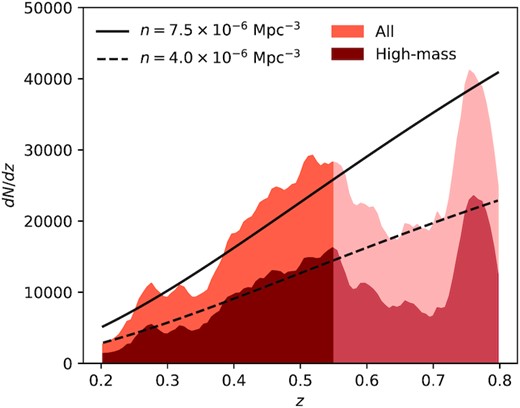
The redshift distributions of the LRG samples studied in this paper. As visible in the figure, the distributions are consistent with the assumption of a constant comoving density up to redshift z = 0.55, the maximum considered in our main analysis. For higher redshifts, we find that the empirical selection criteria explicitly designed to select for a constant comoving density do not hold. We use the high-redshift tail of our LRG sample (All, z > 0.75) to investigate the behaviour of our measurements in this regime.
3 PROFILES
In this section, we discuss how we used our data sets to produce two stacked signals measured around the LRGs: the galaxy profile, capturing the distribution of fainter red galaxies, and the weak lensing profile, a measure of the projected mass distribution extracted from the distorted shapes of background galaxies. We present these two profiles and the 68 per cent contours of two separate parametric fits in Fig. 3. The details of the fitting procedure are explained in Section 4.
3.1 Galaxy profile
We expect bright LRGs to be surrounded by fainter satellites, i.e. we expect them to be the central galaxies of galaxy groups or clusters. To obtain the projected number density profile of the surrounding KiDS galaxies, we split the LRG samples in seven redshift bins of size δz = 0.05 in the range z ∈ [0.2, 0.55]. We then defined a corresponding KiDS galaxy catalogue for each redshift bin, obtained the background-subtracted distribution of these galaxies around the LRGs, and finally stacked these distributions using the weights wi defined below.
We did not select the KiDS galaxies by redshift due to their large uncertainty. Instead, we created one KiDS catalogue for each redshift bin by applying two redshift-dependent selections to the entire catalogue: a lower limit in magnitude and a sample selection in colour space. The reason behind the first selection is simple: in order to identify populations with the same intrinsic luminosity as a function of redshift, a redshift-dependent magnitude threshold is necessary (as suggested by More et al. 2016). On the other hand, the colour cut has a more physical explanation. Red satellites are the most abundant population in galaxy clusters and, due to their repeated orbits inside the host cluster, they are known to better trace dynamical features such as splashback (see e.g. Baxter et al. 2017). Combining these two criteria also has the effect of selecting a similar population even in the absence of k-corrected magnitudes.
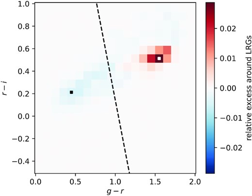
Separating red and blue galaxies. We calculated the distribution of KiDS galaxies in the (g-r)-(r-i) colour plane for objects around random points in the sky and around LRGs in the high-mass sample between redshifts 0.3 and 0.35 (R < 1 Mpc). This histogram represents the difference between the two distributions as a fraction of the entire KiDS population. The black and white squares mark the pixels with the lowest and highest value. An overdensity of red objects and an underdensity of blue objects is apparent, and the line separating the two locations is used to split the full KiDS sample into two populations.
The left-hand side of Fig. 3 presents our measurement of the galaxy profile around the LRGs. As expected, the high-mass subsample has a higher amplitude compared to the entire sample.
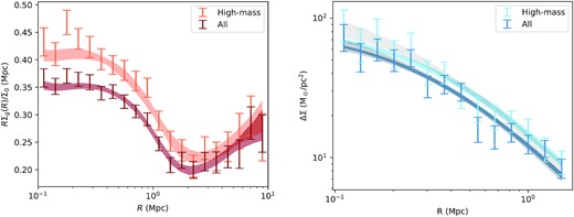
The signals studied in this paper. We measure the number density of KiDs red galaxies (left-hand panel) and the lensing signal (right-hand panel) around the LRGs in our sample (all) and its high-luminosity subsample (high-mass). Both measurements are based on the KiDS photometric catalogue. The steep drop around 1 Mpc visible in the left-hand panel is the splashback feature, and it is connected to the total mass of the LRG haloes. Similarly, the amplitude of the lensing signal on the right is also a measure of the same mass. In addition to the data and the 1σ error bars, we also display the 68 per cent contours of two profile fits performed to extract the mass measurements. The fit on the right is performed either by varying only the amplitude of the signal (thinner contours) or by varying its amplitude and concentration (wider contours). See the text for more details. Section 2 presents the data and the two samples, Section 3 discusses how the profiles are measured, and Section 4 discusses the fitting procedure.
3.2 Weak lensing profile
The shapes of background sources are deformed, i.e. lensed, by the presence of matter along the line of sight. In the weak lensing regime, this results in the observed ellipticity |$\boldsymbol {\epsilon }$| of a galaxy being a combination of its intrinsic ellipticity and a lensing shear. If we assume that the intrinsic shapes of galaxies are randomly oriented, the coherent shear in a region of the sky can therefore be computed as the mean of the ellipticity distribution.
Consider a circularly symmetric matter distribution acting as a lens. In this case, the shear only contains a tangential component, i.e. the shapes of background galaxies are deformed only in the direction parallel and perpendicular to the line in the sky connecting the source to the centre of the lens. Because of this, we can define the lensing signal in an annulus of radius R as the average value of the tangential components of the ellipticities ϵ(t). The next few paragraphs provide the details of the exact procedure we followed to measure this lensing signal around the LRGs in our samples. For this second measurement, we used the weak lensing KiDS source catalogue extending up to redshift z = 1.2 (see also Viola et al. 2015; Dvornik et al. 2017).
The covariance matrix of this average lensing signal was extracted through bootstrapping, i.e. by resampling 105 times the 1006 1 × 1 deg2 KiDS tiles used in the analysis. This signal, like the galaxy profile before, is also statistics limited. Therefore, we have not included the negligible off-diagonal terms of the covariance matrix in our analysis.
Finally, we note that we have thoroughly tested the consistency of our lensing measurement. We computed the expression in equation (8) using the cross-component ϵ(×) instead of the tangential ϵ(t) and verified that its value was consistent with zero. Similarly, we also confirmed that the measurement was not affected by additive bias by measuring the lensing signal evaluated around random points.
4 THREE WAYS TO MEASURE CLUSTER MASSES
This section presents three independent measures of the total mass contained in the LRG haloes. We refer to these estimates as splashback (or dynamical) mass, lensing mass, and abundance mass. The first two are extracted by fitting parametric profiles to the two signals presented in the previous section (Fig. 3), and the third is based on a simple abundance matching argument. Fitting the galaxy profile allows us to constrain the splashback feature and provides a dynamical mass, while fitting the amplitude of the lensing signal provides a lensing mass.
4.1 Splashback mass
Thanks to the splashback feature, it is possible to estimate the total halo mass by fitting the galaxy distribution with a flexible enough model. The essential feature that such 3D profile, ρ(r), must capture is a sudden drop in density around r200m. Its most important parameter is the point of steepest slope, also known as the splashback radius rsp. Equivalently, this location can be defined as the radius where the function dlog ρ/dlog r reaches its minimum.
These expressions define a profile with two components: an inner halo and an infalling region. The term ρEin(r)ftrans(r) represents the collapsed halo through a truncated Einasto profile with shape parameter α and amplitude ρs (Einasto 1965). The parameters g, β in the transition function determine the maximum steepness of the sharp drop between the two regions, and rt determines its approximate location. Finally, the term ρout(r) describes a power-law mass distribution with slope se and amplitude |$\bar{\rho }$|, parametrizing the outer region dominated by infalling material. For more information about the role of each parameter and its interpretation, we refer the reader to Diemer & Kravtsov (2014), and previous measurements presented in the introduction (see e.g. Contigiani et al. 2019b, for more details about the role of the truncation radius rt).
This profile is commonly used to parametrize mass profiles but is used in this section to fit a galaxy number density profile. When performing this second type of fit, the amplitudes ρs and |$\bar{\rho }$| are dimension-less and, together with the flexible shape of the profile, completely capture the connection between the galaxy and matter density fields. Similarly to Σ0, the value of these constants is not the focus of this paper.
To extract the location of the splashback radius for our two LRG samples, we fitted this model profile to the correlation function data using the ensemble sampler emcee (Foreman-Mackey et al. 2013). The priors imposed on the various parameters are presented in Table 1, and we highlight in particular that the range for α is a generous scatter around the expectation from numerical simulations (Gao et al. 2008). The best-fitting profiles extracted from this procedure are shown in Fig. 3.
The priors used in the fitting procedure of Section 4. When fitting the data in the left-hand panel of Fig. 3, we employ the model in equation (11) with the priors presented above. For some parameters, we impose flat priors in a range, e.g. [a, b], while for others we impose a Gaussian prior |$\mathcal {N}(m, \sigma)$| with mean m and standard deviation σ. We do not restrict the prior range of the two degenerate parameters |$\bar{\rho }$| and r0.
| Parameter | Prior |
|---|---|
| α | |$\mathcal {N}(0.2, 2)$| |
| g | |$\mathcal {N}(4, 0.2)$| |
| β | |$\mathcal {N}(6, 0.2)$| |
| rt/(1 Mpc) | |$\mathcal {N}(1, 4)$| |
| se | [0.1, 2] |
| Parameter | Prior |
|---|---|
| α | |$\mathcal {N}(0.2, 2)$| |
| g | |$\mathcal {N}(4, 0.2)$| |
| β | |$\mathcal {N}(6, 0.2)$| |
| rt/(1 Mpc) | |$\mathcal {N}(1, 4)$| |
| se | [0.1, 2] |
In clusters, the location of the central galaxy might not correspond to the barycenter of the satellite distribution. While this discrepancy is usually accounted for in the modelling of the projected distribution in equation (10), we chose not to consider this effect in our primary analysis. This is justified by the fact that the mis-centring term affects the profile within R ∼ 0.1 Mpc, while we are interested in the measurement around R ∼ 1 Mpc (Shin et al. 2021), and the data do not require a more flexible model to provide a good fit.
Finally, to transform the rsp measurements into a value for M200m, we used the relations from Diemer (2020a), evaluated at our median redshift of |$\bar{z}=0.44$|. In this transformation, we employed the suggested theoretical definition of splashback, based on the 75th percentile of the dark matter apocentre distribution. In the same paper, this definition of splashback based on particle dynamics has been found to accurately match the definition based on the minimum of log ρ/log r used in this work. For more details about the relationship between these two definitions, we refer the reader to section 3.1 of Contigiani et al. (2021).
Because the splashback radius depends on accretion rate, we used the median value of this quantity as a function of mass as a proxy for the effective accretion rate of our stacked sample. We note, in particular, that the additional scatter introduced by the accretion rate and redshift distributions is expected to be subdominant given the large number of LRGs we have considered.
4.2 Lensing mass
We point out that we did not use the complex model of equation (11) for the lensing measurement. This is because, the differences between the Einasto profile used there and the NFW profile presented above are not expected to induce systematic biases at the precision of our measurements (see e.g. Sereno, Fedeli & Moscardini 2016). Although extra complexity might not be warranted, particular care should still be taken when measuring profiles at large scales, where the difference between the more flexible profile and a traditional NFW profile is more pronounced. Consequently, we reduce any bias in our measurement by fitting only projected distances R < 1.5 Mpc, where the upper limit is decided based on the rsp inferred by our galaxy distribution measurement.
Since the mass and concentration of a halo sample are related, several mass–concentration relations calibrated against numerical simulations are available in the literature. For the measurement presented in this section, we used the mass–concentration relation of Bhattacharya et al. (2013). However, because this relation is calibrated with numerical simulations based on a different cosmology, we also fit the lensing signal while keeping the concentration as a free parameter. This consistency check is particularly important because halo profiles are not perfectly self-similar (Diemer & Kravtsov 2015) and moving between different cosmologies or halo mass definitions might require additional calibration. We perform the fit to the profiles in the right-hand panel of Fig. 3 using the median redshift of our samples, |$\bar{z}=0.44$|. We find that statistical errors dominate the uncertainties, and we do not measure any systematic effect due to the assumed mass–concentration relation.
4.3 Abundance mass
In addition to the two mass measurements extracted from the galaxy and lensing profiles, we also calculated masses using an abundance matching argument.
The comoving density of haloes of a given mass is a function of cosmology (Press & Schechter 1974). Since we expect a tight relationship between the mass of a halo and the luminosity of the associated galaxy, any lower limit in the first can be converted into a lower limit in the second. Therefore, our measurement of the comoving density in Fig. 1 can be converted into a mass measurement. We note, in particular, that this step assumes that Vakili et al. (2020) built a complete sample of LRGs with no contamination and that the luminosity estimates obtained in Fortuna et al. (2021) are accurate, at least in ranking.
We used the mass function of Tinker et al. (2008) at the median redshift |$\bar{z}=0.44$| to convert our fixed comoving densities into lower limits on the halo mass M200m. To complete the process, we then extracted the mean mass of the sample using the same mass function.
The relation between halo mass and galaxy luminosity is not perfect, however, since the galaxy luminosity function is shaped by active galactic nuclei activity and baryonic feedback. These processes induce an increased scatter in the stellar mass-halo mass relation (Genel et al. 2014), which we have not accounted for. This effect, combined with the uncertainties in the LRG selection and luminosity fitting, are the main sources of error for our abundance matching mass. Since we have not performed these steps in this work, however, we decided not to produce an uncertainty for this measurement and report it here without an error bar. For the same reason, we also do not explore the effect of the slightly different cosmology assumed by Tinker et al. (2008) and the one used here.
5 DISCUSSION
In this section, we compare and validate the measurements presented in the previous one. As an example of the power granted by multiple cluster mass measurements from the same survey, we also present an interpretation of these measurements in the context of modified theories of gravity.
In Fig. 4 and Table 2, we present the results of our two main mass measurements combined with the abundance-matching estimate introduced in the previous subsection. All measurements are in agreement, providing evidence that there is no significant correlation between the selection criteria of our LRG sample and the measurements performed here. The inferred average splashback masses of our LRG samples have an uncertainty of around 50 per cent.
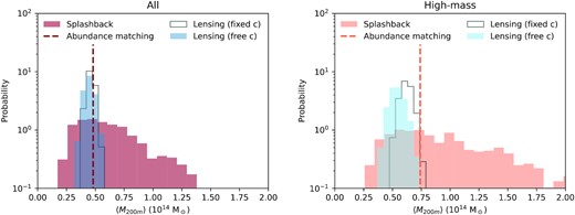
Comparison of the mass measurements performed in this paper. Using three different techniques, we measured the mass of the haloes hosting our LRG sample (all) and a high-luminosity subsample (high-mass). The remarkable consistency between the three methods for both samples is a testament to the robustness of our LRG selection and the prospect of measuring halo masses from the splashback feature. Table 2 reports the same results in textual form. See Section 5 for more details about this comparison.
The mass measurements performed in this paper. This table summarizes the discussion of Section 5 and the measurements presented in Fig. 4 for our LRG samples (all and high-mass). The quoted splashback radii are in comoving coordinates. The abundance-matching measurements are provided without error bars as we have not modelled the selection function of our LRGs. Most measurements and conversions between M200m and rsp are computed using a model at the median redshift |$\bar{z}=0.44$|, identical for both samples (see the end of Section 4.1 for details).
| Technique | M200m (1014 M⊙) | rsp (Mpc) | ||
|---|---|---|---|---|
| All | High-mass | All | High-mass | |
| Splashback | |$0.57^{+0.36}_{-0.21}$| | |$0.9^{+0.85}_{-0.38}$| | 1.48 ± 0.2 | 1.68 ± 0.28 |
| Lensing (fixed c) | 0.46 ± 0.03 | 0.62 ± 0.05 | 1.40 ± 0.01 | 1.52 ± 0.02 |
| Lensing (free c) | 0.44 ± 0.05 | 0.54 ± 0.07 | 1.39 ± 0.03 | 1.6 ± 0.04 |
| Abundance | 0.48 | 0.74 | 1.42 | 1.6 |
The first striking feature is the varying degree of precision among the different measurements. The lensing result is the most precise, even when the concentration parameter is allowed to vary. In particular, the fact that the inferred profiles do not exhaust the freedom allowed by error bars in the right-hand panel of Fig. 3 implies that our NFW model prior is responsible for the strength of our measurement and that a more flexible model will result in larger mass uncertainties. On the other hand, with splashback, we can produce a dynamical mass measurement without any knowledge of the shape of the average profile.
There is also a second, more important, difference between the two measurements that we want to highlight here. The SNR of the splashback mass is dominated by high-redshift LRGs since |$\text{SNR}\sim \sqrt{N_\text{LRG}}$|. While the ability to capture intrinsically fainter objects at low redshift might affect this scaling, we point out that the redshift-dependent magnitude cut introduced in equation (2) explicitly prevents this. In contrast, the lensing weights in equations (6) imply that the more numerous high-redshift objects do not dominate the lensing signal. This is due to a combination of the lower number of background sources available, the lower lensfit weights associated with fainter sources, and the geometrical term in equation (7).
This point is explored quantitatively in Fig. 5, where we compare the two techniques for different redshift bins. The top panel is a projection of the left-hand panel of Fig. 4 in terms of rsp, while the other two are new results. These new measurements at higher redshift are obtained using the same methods presented in Section 3. To be precise: for the galaxy distribution, we impose a 10 SNR cut for the KiDS galaxies and a subsequent colour selection in the (i − Z) − (r − i) plane; while for the lensing signal, we use the same source selection presented before. As visible in the figure, both measurements degrade for higher redshifts, but the two scale differently. If we consider the size of the 68 percentile intervals for the two measurements, at z = [0.2, 0.5] we obtain a ratio between the two of 1:7, while at z = [0.65, 0.7] we obtain a ratio of 1:2.5, significantly better. We point out that these results are not part of our main analysis because of the problems encountered in Section 2.2 when building a high-z selection. However, as discussed in a future section, the different scaling highlighted here has important implications for future photometric missions.
![Galaxy distribution measurements scale better with redshift compared to lensing measurements. The three panels show the posterior distribution of rsp obtained with the two techniques discussed in this paper for three different redshift ranges. The coloured error bars indicate the 68 percentile interval of each distribution. From top to bottom the ratio between the intervals for the two techniques increases significantly: [0.15, 0.25, 0.4], proving the presence of a different redshift dependence that benefits the galaxy distribution measurement. Note that this figure uses rsp as a comparison variable instead of the mass used in Fig. 4. This choice is due to the smaller error bars for this parameter. See the final paragraph of Section 4.1 for more details about how the one-to-one transformation between these two variables was obtained.](https://oup.silverchair-cdn.com/oup/backfile/Content_public/Journal/mnras/518/2/10.1093_mnras_stac3027/1/m_stac3027fig5.jpeg?Expires=1750705401&Signature=BHi23v~kEEOY8qdoVnsb6y5KSIw0WDv8yerpp4bqpmDsQJsmHYMVQE4TENJFs3QKC4MKGGj-QtSvtIymxql1KyOiJ-RF3ZJ47ggBTbe~3UKZrgYpwixAVwqK8qDQ2Q4Gk0lbmROFxDWslVZldRSHuYhsBk1qeHNvMN58jJ75O6gpPynjTlLeeII2wURdsECWOclsnT1IL3BtnwwBs4Hr14p8PXzRPxA~DxLBjOArbwVmyU7pzkAdooDAZhKfjNDuLyPqJft6JoyWwULDYmCIEGgo6ODtRf~K76X0jCAZQZBMWkMH8OdK4DO6Fex8GFzVhmo~~vpw2NwvztLIycFIKQ__&Key-Pair-Id=APKAIE5G5CRDK6RD3PGA)
Galaxy distribution measurements scale better with redshift compared to lensing measurements. The three panels show the posterior distribution of rsp obtained with the two techniques discussed in this paper for three different redshift ranges. The coloured error bars indicate the 68 percentile interval of each distribution. From top to bottom the ratio between the intervals for the two techniques increases significantly: [0.15, 0.25, 0.4], proving the presence of a different redshift dependence that benefits the galaxy distribution measurement. Note that this figure uses rsp as a comparison variable instead of the mass used in Fig. 4. This choice is due to the smaller error bars for this parameter. See the final paragraph of Section 4.1 for more details about how the one-to-one transformation between these two variables was obtained.
As a final note on our main results, we point out that the difference between the masses of the two samples (all and high-mass) is 2σ for the lensing measurement, but it is not even marginally significant for the splashback values (due to the large error bars). As already shown in Contigiani et al. (2019b), splashback measurements are heavily weighted towards most massive objects. To produce a non-mass-weighted measure of the splashback feature, it is necessary to rescale the individual profiles with a proxy of the halo mass. However, because the study of rsp as a function of mass is not the main focus of this work, we leave this line of study open for future research.
5.1 Gravitational constants
In this subsection, we discuss how the combination of the lensing masses and splashback radii measured here can be used to constrain models of gravity. Due to the wide scope of the theories considered, we limit this discussion to a brief introduction and choose to focus primarily on the physical interpretation of our measurements. For additional details about the models, we refer the reader to the references provided in the text.
The principle behind this constraint is the fact that, while General Relativity (GR) predicts that the trajectories of light and massive particles are affected by the same metric perturbation, extended models generally predict a discrepancy between the two.
In high-density regions such as the Solar System, the expectation γ = 1 must be recovered with high precision. Hence, alternative theories of gravity commonly predict scale- and density-dependent effects, which cannot be captured through constant values of μ and Σ. Because rsp marks a sharp density transition around massive objects, it is more suited to test these complicated dependencies. To provide an example of the constraints possible under this second, more complex, interpretation, we followed Contigiani et al. (2019a) to convert the effects of an additional scale-dependent force (also known as a fifth force) on the location of the splashback radius rsp. In particular, the model we employed is an extension of self-similar spherical collapse models and neglects any non-isotropic effects, e.g. those introduced by mis-centring and halo ellipticity.
In the context of symmetron gravity (Hinterbichler et al. 2011), the change in rsp introduced by the fifth force is obtained by integrating the trajectories of test particles in the presence or absence of this force. In total, the theory considered has three parameters: (1) λ0/R(t0), the dimension-less vacuum Compton wavelength of the field that we fix to be 0.05 times the size of the collapsed object; (2) zSSB, the redshift corresponding to the moment at which the fifth force is turned on in cosmic history, that we fix at zSSB = 1.25; and (3) f, a dimension-less force-strength parameter that is zero in GR. The choices of the fixed values that we imposed are based on physical considerations due to the connection of these gravity models to dark energy while maximizing the impact on splashback. See Contigiani et al. (2019a) for more details.
5.2 Future prospects
Our results show that the precision of the recovered splashback mass is not comparable to the low uncertainty of the lensing measurements. Because of this, every constraint based on comparing the two is currently limited by the uncertainty of the first. While this paper’s focus is not to provide accurate forecasts, we attempt to quantify how we expect these results to improve in the future with larger and deeper samples. In particular, we focus our attention on wide stage-IV surveys such as Euclid (Laureijs et al. 2011) and Legacy Survey of Space and Time (LSST; LSST Science Collaboration 2009).
First, we investigate how our results can be rescaled. In the process of inferring M200m from rsp, we find that the relative precision of the former is always a multiple (3–4) of the latter. This statement, which we have verified over a wide range of redshifts (z ∈ [0, 1.5]) and masses (M200m ∈ [1013, 1015] M⊙), is a simple consequence of the low slope of the M200m − rsp relation. Secondly, we estimate the size of a cluster sample we can obtain and how that translates into an improved errorbar for rsp. LSST is expected to reach 2.5 magnitudes deeper than KiDS and to cover an area of the sky 18 times larger (LSST Science Collaboration 2009). Part of this region is covered by the Galactic plane and will need to be excluded in practice, but the resulting LRG sample will reach up to z ∼ 1.2 and cover a comoving volume about a factor 100 larger than what is considered in this work. Because the selected LRGs are designed to have a constant comoving density, we can use this estimate to scale the error bars of our galaxy profile measurement. A sample N = 100 times the size would result in a relative precision in rsp of about 2.5 per cent, which translates into a measured M200m below 10 percentage points. This result is obtained by simply re-scaling the error bars of the galaxy profiles by a factor |$\sqrt{N} = 10$|, but we stress that the effects do not scale linearly for rsp due to the slightly skewed posterior of this parameter. While this uncertainty is still larger than what is allowed by lensing measurements, we point out that this method can easily be applied to high-redshift clusters, for which lensing measurements are difficult due to the fewer background sources available (see Fig. 1).
We note that this simple forecast sidesteps a few issues. Here we consider three of them and discuss their implications and possible solutions. (1) At high redshift, colour identification requires additional bands, as the 4000 Å break moves out of the LSST grizy filters. Additional photometry might be required to account for this and to produce an accurate redshift-dependent selection throughout the entire volume covered by the survey. (2) Even if we assume that an LRG sample can be constructed, the population of orbiting satellites at high redshift might not necessarily be easy to identify as the red sequence is only beginning to form. Ideally, there is always a colour–magnitude galaxy selection that provides a profile compatible with the dark matter profile, but, at this moment, further investigation is required. (3) Finally, with more depth, we also expect fainter satellites to contribute to the galaxy profile signal, but the details of this population for large cluster samples at high redshift are not known. A simple extrapolation of the observed satellite magnitude distribution implies that the number of satellites forming the galaxy distribution signal might be enhanced by an additional factor 10, reducing the errors in mass to a few percentage points. This, however, is complicated by the fact that different galaxy populations might present profiles inconsistent with the dark matter features (O’Neil et al. 2022).
In addition to the forecast for the galaxy profiles discussed above, we also expect a measurement of rsp with a few percentage point uncertainty directly from the lensing profile (Xhakaj et al. 2020). This precision will only be available for relatively low redshifts (z ∼ 0.45), enabling a precise comparison of the dark matter and galaxy profiles. This cross-check can also be used to understand the effects of galaxy evolution in shaping the galaxy phase-space structure (Shin et al. 2021) and help disentangle the effects of dynamical friction, feedback, and modified models of dark matter (Adhikari, Dalal & Clampitt 2016; Banerjee et al. 2020).
6 CONCLUSIONS
Accretion connects the mildly non-linear environment of massive haloes to the intrinsic properties of their multistream regions. In the last few years, precise measurements of the outer edge of massive dark matter haloes have become feasible thanks to the introduction of large galaxy samples and a new research field has been opened.
In this paper, we have used the splashback feature to measure the average dynamical mass of haloes hosting bright KiDS LRGs. To support our result, we have validated this mass measurement using weak lensing masses and a simple abundance-matching argument (see Fig. 4 and Table 2).
The main achievement that we want to stress here is that these self-consistent measurements are exclusively based on photometric data. In particular, the bright LRG samples used here can be easily matched to simulations, offer a straightforward interpretation, and, in general, are found to be robust against systematic effects in the redshift calibration (Bilicki et al. 2021). This is in contrast to other dynamical mass results presented in the literature: such measurements are based on expensive spectroscopic data (see e.g. Rines et al. 2016) and are found to produce masses higher than lensing estimates (Herbonnet et al. 2020), an effect which might be due to systematic selection biases afflicting these more accurate measurements (Old et al. 2015).
Because the relation between rsp and halo mass depends on cosmology, this measurement naturally provides a constraint on structure formation. In this work, we have shown how the combination of splashback and lensing masses has the ability to constrain deviations from GR and the presence of fifth forces (see Section 5.1).
Although the precision of the splashback measurement is relatively low with current data, trends with redshift, mass, and galaxy properties are expected to be informative in the future (Xhakaj et al. 2020; Shin et al. 2021). Next-generation data will enable new studies of the physics behind galaxy formation (Adhikari et al. 2021), as well as the large-scale environment of massive haloes (Contigiani et al. 2021). As mentioned in Section 5.2, stage IV surveys will substantially advance these new research goals. In particular, we have shown that splashback masses scale purely with survey volume, unlike lensing. This implies that this technique is uniquely positioned to provide accurate high-redshift masses.
ACKNOWLEDGEMENTS
OC is supported by a de Sitter Fellowship of the Netherlands Organization for Scientific Research (NWO) and by the Natural Sciences and Engineering Research Council of Canada (NSERC). HH, MCF, and MV acknowledge support from the Vici grant No. 639.043.512 financed by the Netherlands Organisation for Scientific Research (NWO). AD is supported by a European Research Council Consolidator Grant No. 770935. ZY acknowledges support from the Max Planck Society and the Alexander von Humboldt Foundation in the framework of the Max Planck-Humboldt Research Award endowed by the Federal Ministry of Education and Research (Germany). CS acknowledges support from the Agencia Nacional de Investigación y Desarrollo (ANID) through FONDECYT grant no. 11191125. All authors contributed to the development and writing of this paper. The authorship list is given in two alphabetical groups: two lead authors (OC, HH) and a list of authors who made a significant contribution to either the data products or the scientific analysis.
DATA AVAILABILITY
The Kilo-Degree Survey data are available at the following link https://kids.strw.leidenuniv.nl/. The intermediate data products used for this article will be shared at reasonable request to the corresponding authors.
Footnotes
However, we stress here that this constraint does not have implications for dark energy, as the model considered is not able to drive cosmic acceleration in the absence of a cosmological constant.
