


ABSTRACT
We study the magnetic activity in the ultrafast rotator dMe HK Aqr using tomography techniques with high-resolution spectroscopy. We aim to characterize how this magnetic activity appears in a regime of very fast rotation without external forces, given that HK Aqr is, very likely, a single star. We find dark spots located at low latitudes. We also detect prominences below the co-rotation radius and at low latitudes, coinciding with the spot latitudes. This apparent low-latitude activity contrasts with what is typically observed in fast rotators, which tend to form large polar spots. Moreover, we detect a stellar flare that produces an enhancement of the continuum and additional emission in the core of most photospheric and chromospheric lines. We find evidence that the flare is ignited above an active region, as seen in solar flares. This means that, with high probability, the flare is initiated by magnetic reconnection in complex active regions. We also present evidence of bulk redshifted velocities of about 15 km s−1 during the rise of the flare, and velocities of 5–10 km s−1 during the decay phase. An estimation of the heating during the flare results in about 200 kK close to the peak and in 100 kK at the end of the observations.
1 INTRODUCTION
From the study of the Sun we know that the magnetic flux created by means of a dynamo action in the interface between the radiative and the convective zone can emerge into the surface and rise up to coronal heights, mainly due to buoyancy. The magnetic activity in the Sun manifests at the surface in the form of relatively cool, dark spots, where the convection is inhibited by the large aggregation of kG magnetic fields (see e.g. Borrero & Ichimoto 2011). When these fields reach the surface in the form of thin flux tubes, they are seen as bright areas called faculae (in the photosphere) or plages (in the chromosphere). Much less evident is the stochastic magnetism (10–100 G fields; e.g. Trujillo Bueno, Shchukina & Asensio Ramos 2004; Trelles Arjona, Martínez González & Ruiz Cobo 2021) that populates most of the solar surface (more than 99 per cent even during the maximum of the activity cycle).
Magnetic fields are also responsible for the accumulations of relatively cold (chromospheric) plasma in the corona, the so-called prominences, when seen off-limb, or filaments, when seen on-disc. They are supposed to maintain these dense structures against gravity and to isolate them from the million degree corona (see e.g. Mackay et al. 2010). Magnetic reconnection (among these active region fields) is responsible for solar flares, events that can release a large amount of energy in a very short interval of time. This energy is mainly transformed into particle acceleration, sometimes ending up in coronal mass ejections into the heliosphere, and emitted as electromagnetic radiation in the whole spectrum, from gamma rays to radio emission (see e.g. Shibata & Magara 2011).
Solar-like activity is known to take place in other (late type) convective stars, for spectral types from G to M. Starspots and prominences in cool stars are nowadays routinely detected and studied using tomography techniques (Semel 1989). Stellar flares, and even superflares several orders of magnitude more energetic than the ones we observe in the Sun have also been widely detected in photometry, very successfully by both the Kepler (e.g. Shibayama et al. 2013) and Tess (e.g. Tu et al. 2020) missions. Only a few stellar flares have been studied with spectroscopy.
Although these magnetic phenomena are dubbed after their solar analogous, they present obvious differences. For example, detected starspots in solar-type stars are often far larger than sunspots and, while sunspots are restricted to latitudes below ±40°, starspots in rapid rotators are very often found at polar regions (see e.g. Strassmeier 2009). On the other hand, stellar prominences are much larger than solar ones and are found at several stellar radii, sometimes coinciding with the co-rotation radius of the star (see e.g. Collier Cameron 2001). Finally, stellar flares, and more importantly superflares, are found to be more frequent than solar ones (Maehara et al. 2012). These differences are a natural consequence of the wide variety of physical conditions (temperature, age, rotation, etc.) that stars harbour, hence the study of magnetic activity in stars other than the Sun entails a potential breakthrough in our understanding of the interplay between magnetic fields and stellar plasmas as a whole.
From the study of stellar magnetism, it is widely accepted that rotation is a fundamental parameter in determining the activity levels in late-type stellar atmospheres (e.g. Reiners et al. 2009, for a review), even for fully convective stars (Wright et al. 2018). The shorter the rotation period, the higher the magnetic activity level of the star. Observing extreme objects is of particular interest to improve our understanding of this relationship. In this work, we study the extremely rapid rotator HK Aqr (GJ 890) that has a period of 0.4 d, more than 60 times the solar rotation rate.
We focus first on the magnetic activity in terms of starspots and prominences to examine the coupling between its very rapid rotation and its convective envelope in the absence of external forces (for main-sequence stars, rapid rotation is often associated with tidally locked binary systems). Previous works on this topic find contradictory results regarding the latitude of the activity of this star. Young et al. (1990), using mainly the information coming from photometric light curves, claim that this star harbours starspots in its polar caps. However, using spectroscopic tomography techniques, Barnes & Collier Cameron (2001) and Barnes, James & Collier Cameron (2004) find the magnetic activity in HK Aqr to be more equatorial. They, however, argue that near-polar, very high latitude spots cannot be discarded given the signal-to-noise ratio of their data. Another possible explanation for these contradictory results is the existence of a magnetic cycle. As is the case in the Sun, the emergence of magnetic flux can vary from higher to lower latitudes as the cycle evolves. But, in any case, the study of how magnetic activity manifests at the surface can give hints on the operating dynamo. For example, a solar-type dynamo in a fast rotator will lead to the formation of active regions closer to the poles since the ascent of magnetic flux from the interior to the surface is dominated by the Coriolis force parallel to the rotation axis and not by the radial buoyancy force (Schuessler & Solanki 1992). HK Aqr has likely not a solar-like dynamo since M dwarfs have deeper convection zones, even turning to fully convective for spectral masses lower than 0.35 M⊙ (HK Aqr mass is 0.57⊙), which can lead to a more distributed dynamo where magnetic fields are created all along the convection zone and hence can appear at all latitudes.
Prominences have been detected in HK Aqr and they are considered to be located at several stellar radii, though always below the co-rotation radius (Byrne, Eibe & Rolleston 1996; Leitzinger et al. 2016). Leitzinger et al. (2016) present indications of large amplitude oscillations (±10 km s−1, similar values to what is observed in solar prominenences). However, these authors point out that their detection is at the limit of their velocity sensitivity and that their result needs to be confirmed. The high cadence of our observations allows us to perform here such investigation.
Secondly, we study in detail a flaring event that we recorded serendipitously with high-cadence, high-resolution spectroscopy. The mechanical energy of a flare can be even two orders of magnitude larger than the radiated one. This is the reason why studying the mass motions due to a flare can provide important insights on its physics. So far, few works with spectroscopy data claim the observation of blue asymmetries of the lines during the first stages of a flare and red asymmetries during the fading, reinforcing the solar analogy of a particle jet ejection due to magnetic reconnection (Houdebine et al. 1993; Montes et al. 1999; Lalitha et al. 2013; Honda et al. 2018). Also, it is important to relate the flare to the underlying photospheric activity. Only Wolter et al. (2008) show evidence of a flare occurring in the quiet photosphere, displaced from the closer active region. In this work, we provide high-resolution tomography to locate the flare ignition and relate it to the underlying photospheric activity. We also study the possible mass motions and heating effects on the whole stellar atmosphere.
2 OBSERVATIONS
On the nights of 2016 August 20, 21, and 22, we obtained spectroscopy of the dMe star HK Aqr using the High Accuracy Radial velocity Planet Searcher (HARPS-North; Cosentino et al. 2012) at the Telescopio Nazionale Galileo (Roque de los Muchachos) with a resolution of R = 115 000. This ultrastable spectrograph, whose main purpose is exoplanet discovery and characterization, covers the wavelengths from 383 to 690 nm. As a result of the good seeing conditions (below 1 arcsec on average, and with minimum values of 0.3 arcsec), we needed an integration time of just 5 min for individual spectra to achieve an acceptable signal-to-noise ratio. We took sequences of spectra from the rise of the star until the end of the night. The data were reduced with the harps-n dedicated software, which takes care of bias subtraction, flat-field and cosmic rays correction, wavelength calibration using ThAr lamps, and order extraction (Sosnowska et al. 2012). We then renormalized the spectrum to the local continuum. Then, we binned four spectral pixels to improve the noise level at 650 nm to ∼3 × 10⁻² Fc, being Fc the local continuum level (S/N = 33). This limits our velocity sampling to ∼1.8 km s−1 at the 650 nm region. Although this noise level is sufficient for H α and some other strong lines, it does not allow us to study the surface activity in single photospheric spectral lines. To overcome this difficulty, we applied the least-squares-deconvolution technique (LSD; Donati et al. 1997) using a Bayesian approach described in Asensio Ramos & Petit (2015). The LSD profile was built with a spectral sampling of 2 km s−1 and with a Kurucz line list for an M0 star having more than 2000 lines. The noise level is reduced to 1.5 × 10⁻³ Fc (S/N = 666).
3 THE MAGNETIC ACTIVITY OF HK AQR
The inference of quantitative information on magnetic fields can only be achieved through spectropolarimetry, i.e. the interpretation of the polarized spectrum of light. Unfortunately, spectropolarimetry is not a photon-efficient technique. As a result, observing the polarization in stars is very challenging. Installation of polarimeters at large aperture telescopes should eventually increase the sample of stars with solar-like dynamos that can be targeted. Alternatively, we can use high-resolution spectroscopy to derive useful qualitative information on their magnetic activity through magnetic proxies, many of them previously tested in the Sun.
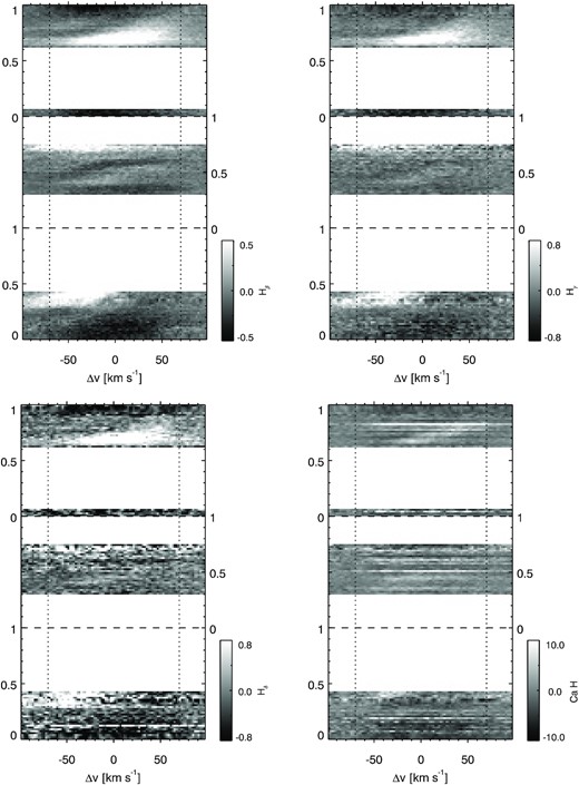
Fig. 1 displays the time evolution of the residual spectra, i.e. Fa − Fq for the photospheric lines and Fa/Fq for the chromospheric ones, where filaments are expected (see more line residuals in A1). The photosphere (left-hand panel) is characterized by the LSD profile computed with many photospheric lines, while the chromosphere (middle panel) is represented here by the H α line. Many absorption and emission tracks are seen both in the photosphere and in the chromosphere, an indication of the presence of solar-like activity features like dark spots, plages, and filaments (prominences). The properties of the track left by activity features in the residual profiles when the star rotates are determined by their position in latitude. A feature at the equator of the star, assuming that the star rotation axis is perpendicular to the line of sight, leaves a track that is seen only during half a the stellar rotation, shifting from blue wavelengths (associated with blueshifted velocities) to red ones. When the feature is placed at higher latitudes, the slope of the track monotonically increases, until reaching the limit when it is located at the pole. In this case, it appears as a vertical feature at zero velocity. Unfortunately, as we will see later, in our observations, the Sun’s spectrum is observed at zero velocity.
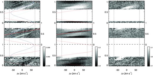
Residuals for the LSD photospheric line (left), the H α line (centre), and the He i D3 line (right). The vertical axis represents the phases during the three nights of observations (separated by the horizontal dashed line). The horizontal axis is the velocity after removing the star’s systemic velocity v⋆ = 6 km s−1 (Barnes & Collier Cameron 2001). Vertical dotted lines display the values of ±vsin i = 70 km s−1 (Barnes & Collier Cameron 2001). Blue lines display the fits to the photospheric spot tracks, while the orange line shows the fit to the track of the prominence as seen in H α.
The unique identification of these tracks with actual features on the surface of the star is not straightforward and it relies on some assumptions. The bright tracks in the LSD line are commonly interpreted in terms of dark (cool, magnetic) spots. This is so, because the continuum flux from a dark spot is lower than that of the quiescent phase and, assuming that the flux of the spectral line formed at the spot is the same as that formed at the quiet surface, the spectral line resulting from the integration of local profiles across the disc has less flux at the velocity (longitude) where the spot is (similar to a planet occultation). In this case, the residual Fa − Fq is positive, i.e. bright in the plot. The identification of bright tracks with dark spots is quite safe since the depth of the lines formed in these cool and largely magnetized areas (the lines broadden due to Zeeman splitting) is typically smaller than the one in quiet areas, which means even less flux at the velocity of the spot. These spots are very likely associated with large accumulations of magnetic flux that inhibit convection and hence appear as cooler than their surroundings, as is the case in the Sun.
Interpreting the dark tracks is more tricky. One can think that these tracks are the footprints of faculae. In the Sun, faculae appear bright in continuum and line wavelengths with respect to the quiet surface. The larger value of the continuum will result in a negative residual (black track) only if the depth of the line is very similar to that of the quiet areas. However, faculae appear bright also in the core of the lines, which would go on the opposite direction. Moreover, faculae on the Sun have only high contrast with the surrounding quiet Sun near the limbs. If this is the case also in HK Aqr, we would expect the tracks more likely visible at the wings of the line. For that reason, the identification of dark tracks in the residual profiles requires a more in-depth study, also considering the effect of having chosen the average profile as the quiescent profile of the star. To study the magnetic activity on the surface of HK Aqr, we focus on the study of starspots since we can safely identify them.
The velocities (minimum position of the absorption Gaussian) associated with the promience track are plotted in the right-hand panel of Fig. 2 versus the phase. As can be seen, the track does not follow the sinusoidal shape, as expected from the previous relation. The explanation of the observed behaviour is as follows. By tracking the velocity at the absorption minima, we are tracking the centroid of the cloud. Imagine now that the cloud has a large extension and has a denser core. When it starts eclipsing the disc, an absorption feature appears in the H α profile centred at the limb velocity. As time passes, more material eclipses the disc and, since the density is larger to the centre of the structure, a larger absoption appears at the limb velocity, hence biasing the velocity to the limb one when computing the minimum of the absorption. This is indeed our case (see Fig. A2). As a result, until most of the material is in front of the disc, the apparent velocity of the cloud is approximately that of the limb. The situation is symmetric when the cloud leaves the other limb. Therefore, when following the centroid of the cloud, we see an almost constant velocity with the phase at the beginning and at the end of the track and, in between, the cloud centroid is reliably tracking stellar rotation (see fig. 7 in Collier Cameron & Robinson 1989). We then select only these points (coloured in black) to fit the track and obtain the height of the structure projected on to the rotation axis. Two extra points at the centre of the track are also avoided since they correspond to a time when the absorption profile of the prominence and the emission one of a spot are in phase. In this case, a lot of degeneracy exists between the parameters of the two Gaussians used to fit the residual profile.
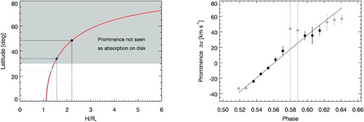
Left-hand panel shows the values of the latitude and the height of the prominence that are compatible with the product (R⋆ + H)cos λ = 2R⋆ obtained fitting the track in H α. The grey area represents the parameter space for which the prominence would not be seen in absorption on disc (i.e. not compatible with our observations). The blue dots correspond to the latitudes inferred for the spots in Fig. 1 and the black line is drawn from the co-rotation radius. Right-hand panel displays the velocity of the residual in H α due to the prominence as computed with Gaussian fits. The vertical lines delimit the |$\overline{\Delta v}\pm 3\sigma$| values. The larger error bars are due to cross-talk between Gaussian functions. Grey dots are not considered for the fit to the track (solid line).
Right-hand panel of Fig. 2 shows the fit to the selected points of the prominence track. Note in Fig. 1 that the same fit reaches velocities larger than vsin i yet the prominence is not seen in emission. This is reasonable since the contrast is very low and only a few prominences have been detected off-limb (Dunstone et al. 2006). Fig. 2 shows the values of the latitude and the height of the prominence that are compatible with the constant (R⋆ + H)cos λ = 2R⋆ obtained by fitting the track. Although all values of height and latitude that satisfy such expression are compatible with the observed track, not all of them are possible. The minimum height of the prominence can be computed by assuming that it lies at the equator. Therefore, the lower limit for the prominence height above the surface is H = 0.78 R⋆. Moreover, we observe the track in absorption, which indeed limits the possible values of latitude and height of the prominence. For the prominences to be seen in absoption, assuming that the rotation axis is in the plane of the sky, the sine of the latitude must lie between zero and the ratio R⋆/(R⋆ + H). The smaller the height of the prominence (H → 0), the larger the range of latitudes available for the prominence (λ → 90°). An upper limit for the maximum latitude available for the prominences is obtained for the minimum height of the prominence. For HK Aqr, from the relation (R⋆ + H)cos λ = 2R⋆, we infer that H/R⋆ ≥ 1 for the cosine to be smaller or equal to one. Therefore, for the minimum height H = R⋆ (lower than the co-rotation height of the star, 2.2 R⋆), we obtain that the upper limit for the maximum latitude available for the prominence is 30°, i.e. a similar latitude than the one of the spots. Therefore, these prominences can be stable only if they are supported against gravity by external forces. In the Sun, prominence plasma is thought to be sustained by local dips of the coronal magnetic field, both in quiet and active regions. In the case of HK Aqr, we speculate that the detected prominence shows a similar phenomenon than a Sun’s active region filament, i.e. chromospheric material suspended at 0.78 − 1R⋆ above the surface held by the magnetic fields connecting the two main active regions observed at the surface and the chromosphere. This idea is reinforced by the fact that the latitude of the dominant spots are compatible with the ones allowed for the prominence and that it is seen in longitudes (phases) in between the two spots (see Fig. 1). The main difference with the solar case would be the height of the structure. While quiescent solar prominences are seen with heights up to 0.14R⊙, active region filaments often lie below 0.014R⊙ (they are indeed not seen as prominences at the solar limb; see e.g. Mackay et al. 2010).
Leitzinger et al. (2016) indicate the possible detection of velocity oscillations of prominences in HK Aqr with a period of 45–50 min. However, they warn about their low signal-to-noise detection. In our case, we do not confirm such detection, as it can be seen in the right-hand panel of Fig. 2. We have similar signal to noise (S/N = 33 in our case and 55 in theirs), but better time cadence (5 min versus 10 min) and spectral resolution (115 000 versus 48 000) than the observations of Leitzinger et al. (2016). The residuals during the passage of the filament are very similar to the ones presented by Leitzinger et al. (2016), most of them being antisymmetric. To fit them they use single and double Gaussians (for the two Gaussians, one in absorption and another one in emission). We instead use three Gaussians (two in emission and one in absorption) since we have realized that these antisymmetric shapes are due to the perturbations produced in the lines by the prominence and the two spots together. For the two spots, we fix the velocities to the ones inferred from the LSD tracks that do not have any contamination (the fits to the residuals can be found in the Appendix). Indeed, the velocities of the spots inferred from the LSD and the H α residuals (with either two or three Gaussians) are very similar in general if we leave the velocities as free parameters, though they differ substantially when the feature of the prominence is present. This is due to the cross-talk between the parameters of the different Gaussians.
4 THE RESPONSE OF THE STELLAR ATMOSPHERE TO A FLARING EVENT
During the last night of observations, a stellar flare was ignited. There are many observables indicating that it is indeed a flare. First, the residuals of the He i D3 line – whose absorption is absent in the star’s quiet chromosphere – show a sudden amplitude increase at the beginning of the third night. In the Sun, this line is present in the absorption spectrum of non-radiatively heated areas, i.e. strongly magnetized active regions or low to medium energy flares (it turns into emission in very energetic ones). This line also presents a weak emission profile in solar spicules and prominences (absorption in filaments). Since HK Aqr does not show any He abundance anomaly, we expect the behaviour of this line to be similar. Therefore, we conclude that the observed He i D3 emission is generated by a very energetic flare.
Further evidence leading to the identification of the flare is the rise and decay of the continuum flux during the event (see Fig. 3). The continuum flux values are rather uncertain because HARPS-N is a fibre-fed spectrograph and the amount of photons collected in each exposure depends on the seeing conditions. Luckily, when the flare occurred at the beginning of the observations the third night, the seeing was extremely good and stable, between 0.3 and 0.5 arcsec (the diameter of the fibre is 1 arcsec). Hence, we can trust the global behaviour of the continuum during the third night, though we cannot rely on the rapid fluctuations or on the comparison among different nights. In the same plot, the right-hand panel shows the time evolution of the blue, green, and red continuum as averaged in a window wavelength around 450, 590, and 690 nm, respectively. In order to decrease the uncertainty due to the wavelength dependance of the seeing and other effects such as differential refraction, camera sensitivity, etc., we divide these continua by its time averaged value when there is no flare (after phase 2.9). As can be seen, the blue continuum has a larger increase than the red one during the flare, which is what we expect in a flare (see e.g. Kleint et al. 2016).
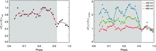
Left-hand panel: ‘White light’ continuum of the third night observations evaluated as an average of the flux of the star between 450 and 450.5, 592.5 and 597.5, 688.0 and 688.3 nm. Right-hand panel: Wavelength average continuum at three spectral windows around 450, 590, and 690 nm. Each average continuum is normalized to the time-averaged values without flare (after phase 2.9). The grey area encloses the time in which the flare is observed.
The emission in the He i D3 line is accompanied by an emission feature in the H α residuals (see Fig. 1). If the continuum around H α were enhanced, but the signal in the line core remained the same, it would result in a negative residual. Therefore, the observed positive residual in H α is compatible with extra emission in the core of the line. The same reasoning applies to the positive residuals found in the Balmer lines (down to H δ), the Ca ii H and K lines, the Mg ı b triplet, the core of the Na i D1 and D2 lines, the He i lines at 447.1, 501.6, and 667.8 nm, the Fe ii line at 516.9 nm, and Fe i lines at 532.8 and 537.1 nm (see Fig. A1 for more details). Interestingly, enhanced positive residuals with respect to the passage of the same spot on the second night are also detected in the average photospheric line (left-hand panel of Fig. 1), which means that most of the photospheric lines have extra emission in the core during the flare (with the limited information we have, the core can be in emission – having a flux larger than the local continuum – or show a self-emission in the absorption profile). In summary, the flare shows a higher value of the visible continumm, extra emission in the cores of the chromospheric H α, H β, and Ca ii H and K and many lines formed in the lower and upper photosphere.
Fig. 4 shows the residuals of the H α and He i D3 lines during the flare. Most of the profiles in Fig. 4 show Gaussian shapes for both H α and He i, even a few that, by eye, seem to have extended blue (dark blue highlighted profile during the rise of H α) or red (light blue highlighted profile) extended tails. The same applies to the rest of spectral lines in which the flare is detected. Therefore, apart from the velocity shift due to stellar rotation, the profiles do not show anomalous shapes typical of local motions of plasma (in contrast to, e.g. Houdebine et al. 1993; Montes et al. 1999; Lalitha et al. 2013; Honda et al. 2018). Note also that the velocity shifts never surpass the vsini, in contrast to other flares reported in the literature for the same star (Byrne et al. 1996). This can be due to the flare occurring at lower atmospheric heights or to a projection effect since plasma flows in flares are highly collimated, or both. Asymmetric profiles are typical in solar flares, i.e. blue asymmetries in H α are frequently observed at the first stages of the flare, while the red asymmetry is mostly associated with the flare ribbons during the impulsive phase (e.g. Berlicki 2007). In stellar flares, many works have claimed detection of blueshifts and redshifts during flare evolution, but we want to warn that all of them rely (as we do) in residual spectra and hence special care has to be taken with their interpretation since the quiescent spectrum is never known with certainty. The fact that we observe mostly Gaussian profiles can be an indication that the strong gradients in the plasma velocity induced by the magnetic field reconnection happens at scales smaller than the flaring area (as is often the case in the Sun).
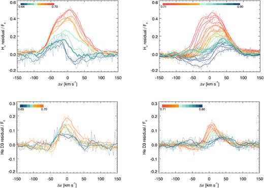
Residual profiles during the rise (left-hand panels) and decay (right-hand panels) of the flare as seen in the H α line (top) and the He i D3 line (bottom). The colours are representative of the phase (see the legend) with the blueish colours during the ignition and the late decay.
Negative features can be seen in the H α residual located towards the red wing of the two first residual profiles and towards the blue wing at the end of the decay phase (see Fig. 4). They can correspond to the end and the beginning of the tracks left by the filaments that transit during the second night (orange line in Fig. 1) and at the end and the beginning of the observations, respectively. A secondary emission appears at the blue wing of H α during the flare decay (at −50 km s−1 highlighted as a light blue profile in the top right panel of Fig. 4). It could also be an absorption appearing at redder wavelengths, or even an active region appearing in the disc, but the fact that it is also seen in the He i D3 (highlighted dark blue profile) makes us think that it is very likely a secondary flare. Secondary flares physically related to the primary event are not uncommon in the Sun and in other flaring stars, and it is also a natural consequence of the standard flare model (Kopp & Pneuman 1976). Note also the brightening at the end of the second night, maybe another flare occurring on the same active region.
In order to infer the velocity and the amplitude and width of the profile due to the flare, we fit the residuals with Gaussian functions. For H α and H β, we assume that the profiles during the flare are a composition of three Gaussians. Two are due to the main and secondary flares and the amplitude are always taken positive, the third is due to the absorption features of prominences and hence always negative. The amplitude, velocity, and FWHM of the two former Gaussians are free parameters. The amplitude and FWHM of the third Gaussian are also free parameters, while the value of the velocity is fixed to the values obtained by fitting the tracks of the prominences. The first residuals of the flare are affected by the prominence that is also visible during the second night, and we use these velocity values (right-hand panel in Fig. 2). The last residuals of the flare are affected by a prominence that is also visible at the beginning of the first night. During this passage, the prominence residuals can be interpreted as a single Gaussian, and we use these values of the velocity. The LSD residuals have been fitted with one Gaussian except for those cases where the secondary flare is evident and we use two Gaussians. The three parameters of both Gaussians have been set free. The rest of spectral lines residuals during the flare are well reproduced with single Gaussian functions.
The velocities of the flare at chromospheric and photospheric heights are displayed in Fig. 5. The velocities inferred from H α, H β, H γ, He i D3, and Ca ii H are very similar, so we average them to reduce the uncertainty (see the Appendix for the tracks in all Balmer lines used as well as in Ca ii H). These are representative of the chromospheric velocity of the flare. The photospheric track is the one of the active region at 25.4° ± 0.9° latitude (see Fig 1). At the end of the decay, the chromospheric velocities coincide with those of the photosphere, i.e. the flare is ignited above the active region. However, interestingly, at the rise of the flare the chromosperic plasma shows redshifted velocities with respect to the photosphere of about ∼5 to 15 km s−1. At the beginning of the decay, the chromospheric redshift is about 10 km s−1 and, as previously stated, it is negligible at the end of the flare decay. Here, we present strong evidence of bulk velocities of chromospheric plasma falling down in response to a flaring event.
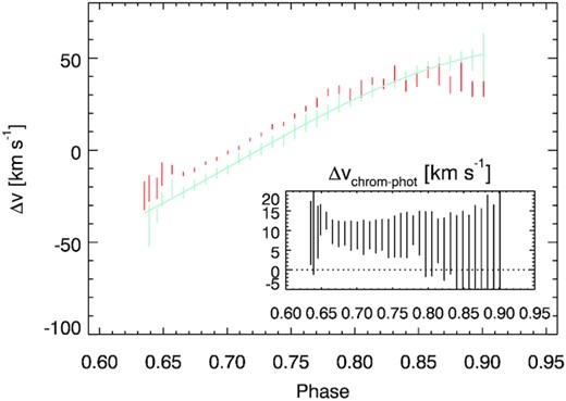
Velocity of the chromospheric residual during the flare (orange) and the LSD one (light blue) that is representative of the photosphere. The inset window is the difference between the chromospheric velocities and the fit to the photospheric ones.
Fig. 6 displays the amplitude of the residuals of different spectral lines during the flare normalized to its maximum value in this period of time. The left-hand panel shows the amplitude of the residual for the Balmer lines and the right-hand panel shows the amplitude for the LSD, the He D3, and the Na D1 lines. The larger error bars in the H α and H β lines are a consequence of the degeneracy of the parameters of a multi-Gaussian fit. The amplitude of the residuals of all spectral lines show a steep increase followed by a slower decay. During the decay phase, in fact, the behaviour of all lines are equivalent within the 3σ level. The secondary flare has an impact in the amplitude inferred for the primary one, likely some degeneracy between the amplitudes of the two Gaussians, both in H α and the LSD residuals. The maximum of the flare occurs at a similar time for all spectral lines, though we are aware that the real peak of the flare is unresolved in time. Kielkopf et al. (2019) report a stellar flare in the M dwarf Proxima Centauri with similar duration as the one detected here. As can be seen in their Fig. 2, the peak of the flare is very short, lasting only for about 200 s. A marginal phase lag exists between the H α and the rest of the lines.
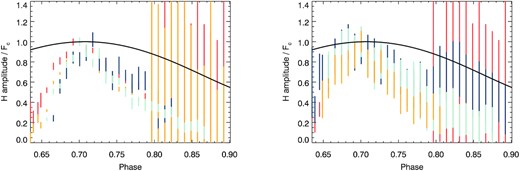
Amplitude of the core emission during the flare in several spectral lines as obtained from the Gaussian fits (with the ±3σ interval as the vertical line. The large errors are due to cross-talk between the parameters of the Gaussian functions. Left-hand panel displays the amplitude for the Balmer lines: H α (orange), H β (yellow), H γ (light blue), and H δ (dark blue). Right-hand panel is the amplitude for the LSD profile (dark blue), the Na D1 line (light blue), and the He i D3 line (yellow) as compared to H α (orange). The black line in both panels is the evolution of the amplitude if the active region is assumed to be circular.
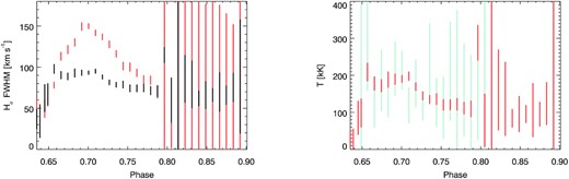
Left-hand panel shows the FWHM of the H α residuals during the flare (black) as compared to their amplitude, both quantities obtained from the fit to Gaussian functions. The vertical lines delimit the average value ±3σ and the larger bars are due to cross-talk between the parameters of the Gaussians. Right-hand panel displays the temperature during the flare as a Doppler velocity dispersion for the H α line (orange) and the He i D3 (light blue).
5 CONCLUSIONS
With high spectral resolution spectroscopy, we find spots at the surface of HK Aqr and prominences embedded in its corona. Both spots and prominences are located at low latitudes, λ = 34° ± 2° and λ = 25.4° ± 0.9° for the spots, and below 29° for the prominences. This finding is consistent with the other tomography study by Barnes & Collier Cameron (2001) and Barnes et al. (2004) but it is in contrast with Young et al. (1990). The interpretation of high latitude spots (Young et al. 1990) was based on light curves and a few spectra of H α whose variation was interpreted in terms of faculae. However, absorptions in the H α line are very likely due to prominences (Collier et al. 1989), hence their conclusions should be revised. Spot patterns in M stars are scarce, but the ones studied so far with the Doppler imaging technique show both high latitude and low latitude spots. As an exception, MNLup shows only low-latitude activity (see Strassmeier 2009).
We cannot rule out the existence of very high latitude spots that leave traces below the present signal-to-noise ratio of our observations (660). However, we want to emphasize that we are able to see by naked eye the very faint (below the noise in individual spectra) track left by the scattered light of the Sun. We are able to see it because the human eye is very good at detecting patterns, and the signal due to the Sun’s spectrum has a large temporal coherence, though in this case, the residual changes sign during the observations and hence cannot be mistaken by a polar spot. Still, we cannot rule out the presence of some near polar activity, though we find very unlikely that large polar spots are present in the star during our observations. An explanation for the lack of polar activity is the presence of an activity cycle that varies the latitude appearance of the spots, as is the case of the Sun (Barnes & Collier Cameron 2001). However, in such a cycle we expect the properties of the stellar atmosphere to vary substantially so that a significant modification of the latitude at which spots emerge, from the poles to ∼20° latitude. In the Sun, the spots appear at latitudes 30°–40° during maxima and at 5°–10° during minima.
We analyse the prominence feature that is seen to fully transit HK Aqr and find that its latitude is consistent with that of the spots and that its height is much lower that the co-rotation radius. This means that an external force must support the relatively cold plasma of the prominence against gravity. Based on the fact that the track of the prominence is in between two tracks left by two spots, we speculate that it is sustained by the magnetic arcade that could link the two active regions.
During the last night, we observed the rise and decay of a very energetic stellar flare. The flare induces an enhancement of the continuum flux and extra emission in the cores of most photospheric and chromospheric lines. Fitting the track of the flare, we find evidence that it is ignited above an active region, as is the case in the Sun (in contrast to Wolter et al. 2008, who find a flare occurring at a quiet region). Therefore, very likely, the flare is the consequence of the magnetic reconnection of the strong fields of the active region. This, in turn, is evidence of complex active regions, i.e. the spot detected can be an unresolved complex dipolar structure, similar to delta-spots on the Sun.
The residual profiles of the flare in all the spectral lines is mostly Gaussian. We have not detected asymmetries like the ones found by other authors (Houdebine et al. 1993; Montes et al. 1999; Lalitha et al. 2013; Honda et al. 2018). The asymmetries in spectral lines are common in solar flares and are due to plasma motions induced by the reconnection event. If those asymmetric profiles exist in the flare of HK Aqr, they are unresolved, the areas having strong velocity gradients being much smaller than the flaring area. We, however, detect bulk velocities during the flare. On average, the chromospheric flaring region is falling towards the surface during the rise phase at about 15 km s−1, and of about 5–10 km s−1 during the decay phase.
The amplitude increase and decay of the extra core emission of photospheric and chromospheric lines is very similar, only the H α line shows evidence of a phase lag, i.e. the amplitude increase happens sooner in H α than in the rest of the lines. The standard deviation of the Gaussian residuals also has a steep increase at the beginning of the flare but a much less pronounced decay as compared to the amplitude. The heating during the flare, as inferred from the width of the H α and He i D3 lines, is about 200 kK close to the peak (the real peak is time unresolved) and decays to 100 kK at the end of the observations.
ACKNOWLEDGEMENTS
This research has been supported by the project PGC-2018-102108-B-100 of the Spanish Ministry of Science and Innovation and by the financial support of M. J. Martinez Gonzalez through the Ramón y Cajal fellowship. We also acknowledge the funding received from the European Research Council (ERC) under the European Union’s Horizon 2020 research and innovation program (ERC Advanced Grant agreement No. 742265). Manuel Luna acknowledges the support from Ministerio de Economia, Industria y Competitividad for the Ramón y Cajal fellowship RYC2018-026129-I. Tobias Felipe acknowledges the financial support from the State Research Agency (AEI) of the Spanish Ministry of Science, Innovation and Universities (MCIU) and the European Regional Development Fund (FEDER) under grant with reference PGC2018-097611-A-I00. Martin Leitzinger acknowledges the Austrian Science Fund (FWF): P30949-N36.
DATA AVAILABILITY
The data analysed in this paper can be found in the Telescopio Nazionale Galileo database. However, if any reader encounters any problem to download them, they can refer to the first author and the data will be provided.
REFERENCES
APPENDIX A: RESIDUALS FOR THE BALMER LINES AND FOR Ca ii H
Residuals for the Balmer lines from H β to H δ and for Ca ii H. The vertical axis represents the phases during the three nights of observations (separated by the horizontal dashed line). The horizontal axis is the velocity after removing the star’s systemic velocity v⋆ = 6 km s−1 (Barnes & Collier Cameron 2001). Vertical dotted lines display the values of ±vsin i = 70 km s−1 (Barnes & Collier Cameron 2001).
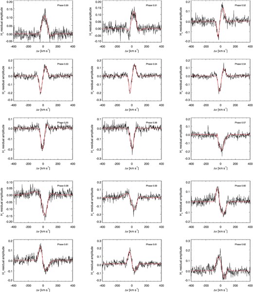
Fits (orange line) to the residuals of the H α line during the transit of the prominence (absorption feature) in the second night. The fits have been obtained using a model with three Gaussians, one in absorption for the prominence and the other two in emission associated with the simultaneous passage of the two spots. The velocities of the spots passage are being fixed and inferred previously from the LSD data (see main text for more details).
