Pulsar emission beam geometry of radio broad-band Arecibo sources^★

ABSTRACT

1 INTRODUCTION

Neutron stars that are detected through pulsed electromagnetic radiation are called pulsars. Radiation from pulsars is generated by plasma flowing along the magnetic field lines (flux tube) near the pulsar polar cap (Ruderman & Sutherland 1975). The physics and dynamics responsible for the plasma outflow and emission from pulsars are still an open and ongoing field of study (e.g. Harding 2018; Melrose 2017; Melrose, Rafat & Mastrano 2020; Cruz et al. 2021); thus, observational characteristics of the emission region are essential in constraining physical theories of the magnetosphere. Regarding radio emission mechanisms, many plausible suggestions have been offered, including streaming instabilities (Melrose 2017; Benáček et al. 2021), orientation of the pair-formation fronts (PFFs; Cruz et al. 2021), and curvature radiation Harding (2018) to name a few. The difficulty remains in assessing that adequately captures all aspects of the radio emission behaviour we observe. One important experimental constraint is the geometry of the radio emission region (hereafter referred to as the emission geometry).

Pulsars possess highly directional radiation beams, as the majority of the radiation generation is confined to the polar flux tube. An observer is limited to seeing intensity along a narrow line-of-sight crossing through this radiation pattern. The projections of the pulsar beam/beams on to an observer’s line of sight are referred to as the main pulse and interpulse. Integrating over a large number of rotations garners a stable measure of the pulsar’s average radiation called the average profile,¹ while substructure in the main pulse and interpulse are called components.

The existence of components and their ordered frequency evolution amongst slower rotation-powered pulsars (hereafter canonical pulsars) provide the strongest evidence for an ordered emission geometry. Additionally, there is strong evidence indicating that the magnetic fields of canonical pulsars are approximately dipolar in the radio emission region (as seen in polarization properties such as Radhakrishnan & Cooke 1969); it is very likely that the orderedness of the presenting emission geometry is intrinsically linked with the presence of field dipolarity. This assumption does not hold for other subpopulations, such as millisecond pulsars (MSPs),² or magnetars. Efforts to quantify pulsar beams and their empirical properties remain a difficult task as we are limited to a confined (and randomized) sightline through each pulsar’s beam configuration. Therefore, investigations have previously proceeded by proposing an underlying emission geometry and then attempting to identify scaling relations using a large ensemble of pulsars. The first beam model consisted of a single hollow cone (Radhakrishnan & Cooke 1969; Komesaroff 1970). Subsequent efforts added a central pencil beam and the possibility of two concentric hollow conical beams (Backer 1976), called the core/double-cone model. Early studies (Cordes, Rankin & Backer 1978) of canonical pulsars suggested that the emission height was correlated with the emitted radiation’s frequency (called radius to frequency mapping). Building on this work, Rankin (1983) identified two different types of frequency evolution that components undergo, and attributed this effect to an ordered evolution of the emission geometry with emission height.

Under this assumption, it is natural to infer that the frequency evolution of pulsar profiles is key to interpreting the underlying emission geometry. However, the majority of pulsars have only been observed within a narrow portion of the radio band. Lower frequency observations are difficult both because of turnovers in pulsar spectra as well as the difficulty of correcting for dispersion smearing caused by the ionized Galactic interstellar medium (ISM; Lorimer & Kramer 2004). In addition, broadening by scattering in the ISM often obfuscates component interpretation. Likewise, the majority of pulsars possess spectra that render them observationally undetectable at higher frequencies, thus limiting the frequency range over which frequency evolution can be detailed. Pulsar beaming studies then have historically focused on determining profile configurations around 1 GHz, including those conducted by Rankin (1993a, b, hereafter ET VIa, ET VIb).

A number of surveys now provide higher quality pulsar profiles that can then be used to study empirical trends over a larger frequency range and better constrain profile classifications. The Pushchino Radio Astronomy Observatory (PRAO) in Russia has long pioneered low-frequency studies of pulsar emission using their DKR-1000 cross telescope at frequencies below 100 MHz and the Large Phased Array instrument at just above 100 MHz. Surveys by Kuz’min & Losovskii (1999, hereafter KL99) and Malov & Malofeev (2010, hereafter MM10) provide a foundation for this work. Similarly, the 25/20-MHz survey by Zakharenko et al. (2013, hereafter ZVK13+) and Kravtsov et al. (2022, hereafter KZU+) using the Giant Ukrainian Radio Telescope (UTR-2) in Kharkiv follows a long record of pioneering pulsar observations in the decametric band. More recently, the Low Frequency Array (LOFAR) in the Netherlands has produced an abundance of high-quality profiles starting with their High Band Survey (hereafter BKK16+, PHS16 + Bilous et al. 2016; Pilia et al. 2016) in the 100–200-MHz band and supplemented by others at lower frequencies (hereafter BKK20++, BGT19 + Bondonneau et al. 2020; Bilous et al. 2020). With respect to high-frequency observations, the most recent example is the Arecibo 4.5-GHz polarimetric single-pulse survey by Olszanski, Mitra & Rankin (2019, hereafter OMR19) following older surveys such as von Hoensbroech & Xilouris (1997, hereafter vHKK97).

Our overall goals of this paper and related papers (e.g. Rankin 2022) are to better understand the spectral changes in emission beam structure and to identify their physical implications. In this paper, we will primarily focus on assessing the efficacy of the core/double-cone beam model over the broadest frequency range yet. We focus on a large group of pulsars within the Arecibo sky that have been studied polarimetrically up to 4.5 GHz (Olszanski et al. 2019) and observed down to 100 MHz or below. These pulsars are well represented in the PRAO, UTR, and LOFAR surveys, and most are seen in earlier surveys as Gould & Lyne (1998, hereafter GL98), Weisberg et al. (1999, 2004, hereafter W99, W04), and Hankins & Rankin (2010, hereafter HR10). Almost all were discovered before 1975 and therefore have ‘B’ names together with a long history of study that we both draw upon and reference as possible. Readers can refer to OMR19 together with these works as needed to familiarize themselves with the basis for our analyses here.

In what follows, Section 2 reviews the geometry and theory of core and conal beams, Section 3 describes how our beaming models are computed and displayed, Section 4 discusses scattering and its effects at low frequency, Section 5 outlines a set of questions about core and conal emission for further consideration, and Section 6 summarizes the results. The main text details our analysis procedures while the tables, model plots, and comments on individual sources are given in Appendix A of supplementary material. The supplementary material also includes ASCII-formatted files corresponding to the three tables.

2 CORE AND CONAL BEAMS

2.1 Pulse profile classification

Canonical pulsar average profiles are observed to have up to five components (Rankin 1983). This places an important constraint on the possible emission-beam configurations. Any beam model we adopt or postulate, must obey the condition that under a line of sight, no more than five components will ever be present in the main pulse. For this paper, we adopt the emission geometry proposed by Backer (1976), which consists of two emission cones surrounding a central core emission beam; known as the core/double-cone model.

Under this model, pulse profiles divide into two major categories depending on which types of emission our line of sight encounters and thus which pulse components are most pronounced in the observed profile. For core profiles there are three types of possible pulse profiles: single (S_t) profiles consisting of an isolated core component,³ triple (T) profiles with a core component flanked by a pair of outriding conal components, or five-component (M) profiles with both an inner and outer pair of conal components and a central core component. By contrast, conal class profiles include conal single (S_d) that is comprised of a melded pair of cones, double profiles (D) consisting of a widely separated pair of conal components occasionally with a weak core component in-between, or rarer intermediate geometries conal triple (cT) or quadruple (cQ) profiles. It should be noted that even if a profile is dominated by core or cone emission components, it does not preclude both from being present in the profile. Even so, the profile classification is important because it is a tracer of the prevalent type of emission encountered as our sightline traverses a pulsar’s radiation beam.

Each profile class tends to evolve with frequency in a characteristic manner: core-single (S_t) profiles often ‘grow’ a pair of conal outriders at high frequency, whereas conal single (S_d) profiles tend to broaden and bifurcate at low frequency.⁴ Triple (T) profiles usually show all three components over a very broad-band, but the relative component intensities can change greatly. Five-component (M) profiles tend to exhibit their individual components most clearly at meter wavelengths; at high frequency, the components often become conflated and at low frequency the inner cone often weakens relative to the outer one.

Also important to the profile class is single-pulse phenomenology. Subpulse drift, a single-pulse phenomenon where emission appears to periodically ‘drift’ across a phase window has long been associated with conal emission and is another criteria in classifying a profile (as an example, see Fig. A13). For a comprehensive review of subpulse drift and associated analyses, we refer the reader to Basu et al. (2019). Highly periodic drifting, as well as other periodic emission can be folded to find an average modulation sequence. This is useful for studying highly periodic phenomena in our single pulses and can be useful in identifying profile substructure that otherwise would be hidden in the average profile. A significant number of pulsars are well modelled by the core/double-cone emission geometry, as described in a continuing series of publications with the overall title Empirical Theory of Pulsar Emission, such as ET VI (Rankin 1993a, b).

These 1-GHz inner and outer conal emission heights have typically been seen to concentrate around 130 and 220 km, respectively. However, it is important to recall that these are characteristic emission heights, not physical ones, estimated using the convenient but perhaps problematic assumption that the emission occurs adjacent to the ‘last open’ field lines at the polar flux tube edge. More physical emission heights can be estimated using aberration/retardation (Blaskiewicz, Cordes & Wasserman 1991 as corrected by Dyks & Harding 2004), and these are typically somewhat larger than the characteristic emission heights.

A number of studies have followed expanding the population of pulsars with classifications. Most have looked at the frequency evolution between |$\tt {\sim }$|300 and |$\tt {\sim }$|1500 MHz in order to model a pulsar’s emission geometry at 1 GHz (Weisberg et al. 1999, 2004; Mitra & Rankin 2011; Brinkman et al. 2018). Olszanski et al. (2019) took a similar approach but extended consideration to 4.5 GHz. Other compendia of polarized pulsar profiles, such as Gould & Lyne (1998), Han et al. (2009), and more recently McEwen et al. (2020) have also been useful.

2.2 Generation of profile types by plasma source

Figure 1.

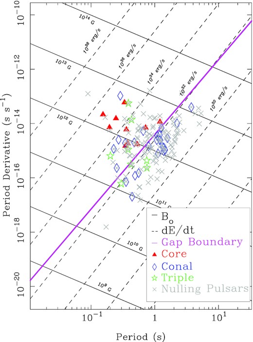
|$P{\!-\!}\dot{P}$| diagram showing the location of core, conal, and triple profiles with respect to the PFF boundary line. Also plotted are pulsars known to null. Core pulsars tend to lie to the upper left of the boundary line while conal emission falls to the lower right (see the text). Triple profiles with their mixture of core and conal emission lie in between. Only one conal source falls significantly far away from the boundary line, J0631+1036. This source provides an example of an unusual cQ profile, and clearly stands out as abnormal compared to the majority of our sources. The great majority of nulling pulsars sit relatively close to the given boundary line.

Open in new tabDownload slide

This division is fundamental to the core/double-cone beam model of ET VI. Pulsars with conal single (S_d), double (D) and five-component (M) profiles tend to fall below the boundary line to the right, whereas those with core-single (S_t) profiles are found to the upper left of the boundary. Those with triple (T) profiles are found on both sides of the boundary. In the parlance of ET VI, the division corresponds to an acceleration potential parameter B₁₂/P² of about 2.5, which in turn represents an energy loss |$\dot{E}$| of 10^32.5 erg s⁻¹. This delineation also squares well with Weltevrede & Johnston’s (2008) observation that high-energy pulsars have distinct properties and Basu et al.’s (2016) demonstration that conal drifting occurs only for pulsars with |$\dot{E}$| less than about 10³² erg s⁻¹.

It is important to point out that the boundary shown in Fig. 1 is a theoretical result and individual pulsars are likely to depart somewhat depending on their own magnetospheric conditions. As a pulsar ages through this threshold, it is reasonable to expect that the emission dynamics would be prone to transitory mixed behaviours such as mode changing, nulling, and amplitude modulation (all indicative of changes in plasma supply and generation). Mode changing in particular alters the core/cone dominance and changes how a profile is interpreted. Strong evidence of this has already been seen in B0823+26, which sits directly on the boundary line and has been one of the best-studied core-single pulsars in the Arecibo sky. Only recently was the pulsar discovered to rarely exhibit a weak second mode,⁶ which features a mainly conal profile (Rankin, Olszanski & Wright 2020)⁷ with traces of core emission, similar to a specific subpopulation of conal profiles (Young & Rankin 2012). Had its secondary emission mode been more frequent, this pulsar might have been classified as conal. It is further worth noting that the great majority of pulsars known to exhibit nulling (Konar & Deka 2019) concentrate around this region of the |$P{\!-\!}\dot{P}$| diagram. Wang, Manchester & Johnston (2007) further studied the nulling fraction, and pulsars with higher nulling fractions appear to lie close to and around this boundary line as shown in their fig. 2. If mode changes are associated with a pulsar’s transition through this boundary, it could explain the odd blending of core/conal/triple profiles we see in Fig. 1, and suggest some of these pulsars have yet to be discovered secondary emission modes.

3 COMPUTATION AND PRESENTATION OF GEOMETRIC MODELS

Two observational values are key to computing conal radii: the profile width and the PPA sweep rate R. The former gives the angular scale of the emission beam, and latter the impact angle β showing how the sightline crosses the beam. Fig. 2 of ET VI depicts this configuration and the spherical geometry underlying the emission.

Empirically, core radiation beams are found to have bivariate Gaussian (von Mises) beamforms such that their invariant widths (full width at half-maximum) measure α but provides no β information. If a pulsar has a core component, we attempt to use its width at around 1 GHz to estimate the magnetic colatitude α, and when this is possible the α value is bolded in Table A3. β is then estimated from α and the PPA sweep rate R at the point of steepest gradient. The outside half-power (3 db) widths of conal components or pairs are measured, and the spherical geometry above then used to estimate the outside half-power conal beam radii. Where α has been measured, that value is used, otherwise a value is estimated by using the established conal radius or characteristic emission height for an inner or outer cone at 1 GHz. These conal radii and core widths are computed for different frequencies where possible.

In most cases, our profile measurements follow closely from those in OMR19 and exhibit 1-GHz geometrical models identical or very similar to those given in their table 6. However, here we extend the analysis using LOFAR High Band 100–200-MHz or Pushchino Observatory 102/111-MHz profiles and in some cases below 100 MHz using LOFAR Low Band, Pushchino, or UTR profiles. Table A1 gives the sources for these profiles in both principal bands as well as each pulsar’s observational parameters. Table A2 gives the physical parameters that can be computed from the period P and spin-down |$\dot{P}$| – that is, the spin-down energy |$\dot{E}$|⁠, spin-down age τ, surface magnetic field B_surf, the acceleration parameter B₁₂/P², and the reciprocal of Beskin, Gurevich & Istomin’s (1993) similar Q (=|$0.5\ 10^{15} \dot{P}^{0.4} P^{-1.1}$|⁠) parameter.

Following the analysis procedures of ET VI, we have measured outside conal half-power (3 db) widths and half-power core widths where useful, using Gaussian fits from Michael Kramer’s bfit code as detailed in Kramer et al. (1994). However, we do not plot these directly. Rather we use the widths to model the core and conal beam geometry in a manner similar to that of OMR19, but here emphasizing as low a frequency range as possible. The model results are given in Table A3 for the 1-GHz band and for the respective 100–200 and <100-MHz band regimes.

We plot our results in terms of core and conal beam dimensions as a function of frequency, as described in Fig. 2. The results of the model for each pulsar are then plotted in Figs A1–A4. For each pulsar the plotted values represent the scaled inner and outer conal beam radii and the core angular width, respectively. The conal beam radii are scaled by a factor of |$\sqrt{P}$| and the core width (diameter) by |$\sqrt{P}\sin {\alpha }$|⁠. This facilitates easy comparison of the beaming models for different objects as well as showing how each evolves with frequency relative to expected 1-GHz dimensions. The outer and inner conal radii are plotted with blue and green lines and the core diameter in red. The nominal values of the three beam dimensions at 1 GHz are shown in each plot by a small triangle.

Figure 2.

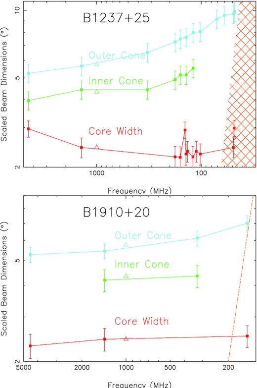
Sample core/double-cone beam model displays for pulsars B1237+25 and B1910+20. Curves for the scaled outer and inner conal radii and core width are shown – the former by |$\sqrt{P}$| and the latter by |$\sqrt{P}\sin \alpha$|⁠. Conal error bars reflect the rms of 10 per cent uncertainties in both the profile widths and PPA rate (see the text), and the core errors also reflect a 10 per cent error. The upper display gives an example of a measured low-frequency scattering level as indicated by the double hatching; whereas the lower display shows 10× the average scattering by the orange (dot–dashed) line. The plots are logarithmic on both axes.

Open in new tabDownload slide

Estimating and propagating the observational errors in the width values is a difficult task as errors can spawn from a variety of different sources. Examples include unknown instrumental errors, issues in interpreting and measuring the profile, inherent effects such as mode changing, to name only a few. Therefore, we have chosen to show error bars reflecting the (scaled) beam-radii ρ_scaled errors for a 10 per cent uncertainty in the width values and a 10 per cent uncertainty in the PPA sweep rate – the former 0.1(1 − β/ρ)ρ_scaled and the latter 0.1(β/ρ)ρ_scaled. The error bars shown reflect the rms of the two sources with the former indicated in the lower bar and the latter in the upper one. For many pulsars, only one of the errors is dominant so the bars corresponding to the two individual error sources are hard to see; however, B1633+24 provides a case where they can be seen quite clearly. The errors shown for the core-beam angular diameters are taken to be 10 per cent in the scaled width.

4 LOW-FREQUENCY SCATTERING EFFECTS

Scattering in the local ISM distorts and broadens profiles by delaying a portion of the pulsar’s signal. This accrues as an exponential tail that can go from being hardly noticeable to dominant within an octave or so due to its steep (f⁻⁴) frequency dependence. Beam modelling relies upon the intrinsic profile dimensions, therefore it is important to include the effects of scattering in our analysis so as to better distinguish intrinsic frequency evolution from scatter broadening.

Many of the pulsars in this group have published scattering or scintillation studies that can be used to estimate the scattering time at a given frequency. We are indebted to Kuz’min & Losovskii (2007) and Kuz’min, Losovskii & Lapaev (2007) for their extensive compendium of 100-MHz scattering times as well as other studies by Alurkar, Bobra & Slee (1986), Geyer et al. (2017), and Zakharenko et al. (2013). We attempt to estimate the regime where scattering significantly contributes to the growth of beam dimensions. In cases where 100 MHz scattering time-scales are available, they are converted to rotational phase and scaled by |$\sqrt{P}$| to make the scattering comparable to core beam dimensions. The frequency evolution is then scaled using an index of −4.1 as adopted by Kuz’min & Losovskii (2007) and are shown on the model plots as double-hatched orange regions where the boundary reflects the scattering time-scale as a function of frequency (see e.g. the model plots in Fig. A1). It is important to emphasize that the scattering time-scale is being plotted alongside the scaled beam dimensions. As cone radii are related to their respective half-power widths through a geometric relationship, the way we have scaled the scattering will make it directly comparable to core widths, while serving only as an estimate for scattering broadening of the conal beam dimensions.⁸ It is also important to note that the scattering line of sight can evolve significantly during time-scales of months/years between observations causing fluctuations around a given mean. It is thus likely that the experimentally measured scattering time-scales we have plotted are not applicable to all of the observation epochs used.

Because of the scattering time-scales dependence, the expected core component beam dimension should show a steady growth towards lower frequencies once past the scattering boundary and equivalently, the conal beam dimensions will also grow.⁹ Generally, the beam dimensions in the scattering regime behave as expected with our expectations for the majority of pulsars studied. Careful attention should be drawn to B0523+11 and B1633+24, where there is no apparent change in beam dimensions even in the scattering regime. We believe that for these cases, it is most likely that the scattering time-scale decreased to a significantly lower value by the time low-frequency observations were taken.

Aside from a few outliers, the majority of inner cones show very little frequency evolution. The outliers can and most likely are explained by misclassification and scattering effects, however at least one appears to be intrinsic (B1237+25). Similarly, the vast majority of outer cones exhibit frequency evolution, while again there are several outlier cases where no frequency evolution is apparent. Core components appear to show no uniform trends.

5 EXPLORING THE PLASMA PHYSICS OF CORE AND CONAL BEAMS

The core/double-cone model has been largely successful in providing a structure for identifying pulsars having similar beam configurations and in giving a basis for estimating a pulsar’s magnetic colatitude α and sightline impact angle β (e.g. ET VI). Practical problems arise with conflated components and difficulties in estimating or interpreting the PPA rate. More significantly, many pulsars with rotational periods of 100 ms or less – and a few with longer periods – have complex profiles that are not well described by the core/double-cone model. One possibility is that conformance to the model requires a dipolar magnetic field in the emission region – and this may well be the case for most slow pulsars at several hundred km emission heights, but not for some faster pulsars where multipole fields cause deformations to the underlying emission geometry.

The larger question is what conformance to the core/double-cone model – seen polarimetrically and across the entire pulsar emission band – implies about the plasma physical processes that underlie the emission seen in these pulsars. One or two sources of e⁻/e⁺ plasma produce the host of fascinating dynamical processes that have been identified over the last half century such as subpulse drifting, mode changing, nulling (e.g. Rankin 1986, ET III), and these in turn generate the profile forms we observe with such effects as antisymmetric V signatures (e.g. ET IV/V, Rankin 1990; Radhakrishnan & Rankin 1990, ET IV/V), edge depolarization (Rankin & Ramachandran 2003, ET VIII), and 90° linear polarization (modal dominance) ‘flips’. These effects are manifested at the radio emission height within the polar flux tube, and apparently this height changes with wavelength as the flux tube opens and B decreases along with both the plasma density and plasma frequency.

Comprehensive analyses and interpretations of radio pulse profile variations with radio frequency are thus crucial. Pulsar beams together with their spectral and polarization changes carry uniquely important information about the geometry of the polar flux tube and plasma physical conditions within that give rise to the radio emissions we receive.

5.1 Core beams

Core components are observed to have a 1-GHz longitude width W_core = 2.45°|$P^{-1/2}\csc \alpha$| reflecting the 2.45°P^−1/2 angular diameter of the polar cap. The 1-GHz core width has proven to be a highly reliable benchmark amid a sea of irregular pulsar parameters (Rankin 1983); however, variations in core widths are observed that are not well understood. For instance, the well-studied B1237+25 has two parts to its core component with the trailing section usually much stronger than the leading, such that its width below in Fig. A2 remains nearly constant. On the other hand, another well-studied pulsar, B0823+26 (Fig. A2) has a core width that seems to increase very substantially at lower frequencies. Given the well-established connection between the core width and the polar cap diameter, any variation in the core width needs improved understanding.

Core components tend to have a distinct asymmetry between their leading and trailing parts. Even those with near Gaussian forms and prominent antisymmetric circular polarization (V) tend to have a discernible asymmetry in the polarization profile. In some, there is further evidence of an early and late orthogonal polarization mode. Further, some core components have substantial linear polarization and PPA traverses that are smooth continuations of adjacent conal components – but in other cases, the PPA appears disordered and linearly depolarized. Isolated cores do not seem to show edge depolarization, and thus conal power may be responsible for any orderly PPA traverse. There is thus much to understand about the polarization of core components and the reader can observe examples of these circumstances as seen in (Olszanski et al. 2019).

Our low-frequency observations can also teach us about the relative RF spectra of the core and conal emission. At high frequencies, core radiation often seems to have a softer spectrum than the conal emission (ET I) in the same pulsar, but it is unknown if that is also true at long wavelengths. We see few clear cases of core emission at very low frequency, but then this is also true for conal radiation, so spectral turnovers must mitigate against both. It will thus be important to pay close attention to pulsars where both survive to low frequencies.

5.2 Inner and outer conal beams

Five-component pulsars tend to have steep PPA sweep rates and small β/ρ that suggests a sightline traverse near the centre of the beam pattern. Such pulsars also permit α to be estimated from the core width, so the conal radii can be computed straightforwardly with spherical geometry as detailed previously. The detailed analyses in ET VI show that the outside half-power radii of the inner and outer cones at 1 GHz for 1-s pulsars are 4.33° and 5.75°, respectively, and that these radii scale in the same manner as the core width – that is, as the inverse square root of the rotational periods (P^−1/2). Remarkably, we further find that (T) pulsars with a single cone and core component – where we can also use the core width to estimate α – clearly fall into two types: those with inner cones and those with outer cones.

A number of questions then devolve from these circumstances, namely why there are two (and only two) types of cones, and what are the geometric and/or physical circumstances that determine these specific conal dimensions. These dimensions point to specific emission heights along particular dipolar field lines within the polar flux tube (e.g. the 130 and 220 km along the flux tube edge as mentioned above), but we do not yet fully understand just why these particular field lines and heights.

One prominent difference between the cones is that inner cone radii tend to change little with frequency, whereas outer cones usually show a strong frequency dependence. The reasons for this wavelength dependence, however, are not well understood.

A complication is that for many pulsars it is difficult to determine whether their cone is an inner or an outer one. If our sightline misses the core beam (or it is absent), we only see a cone. For a pulsar like B1133+16 (see Fig. A2) that shows a large increase in cone size with wavelength, we tend to assume it is an outer cone; whereas for pulsars like B0834+06 or B1919+21 (Figs A2 and A3) their lack of growth over a very large band suggests inner cones.¹⁰ A remarkable effect seemingly seen in both types of cones is edge depolarization: it appears that the outer edges of many conal components are depolarized by equal amounts of modal polarization (ET VIII). We see this in both inner and outer cones when they occur on their own. However, in configurations where both the inner and outer cone are present, the depolarization is seen on the outer cone but not the inner. The depolarization is often complete on the extreme outer edges, so this must involve a strong physical principle. Related to this is the circumstance that many conal single profiles – where the sightline is tangential – are highly depolarized; whereas those involving a more central sightline traverse show more linear polarization.

A final mystery is that the inner and outer cones do not seem to represent fully independent emission. In configurations where subpulse drifting can be observed in both cones simultaneously (usually conal triple or quadruple profiles), the rotating ‘beamlets’ seem to maintain a similar spacing and phase in each cone (e.g. Hankins & Wolszczan 1987).

6 SUMMARY

We begin a process of examining how pulsar beams appear at lower frequencies and interpreting these changes in terms of the pulsar emission geometry. Explicitly, we assume the emission geometry for canonical pulsars is comprised of a core/double-cone beam. Here, we consider a group of well-studied pulsars within the Arecibo sky. This group also includes most of the Arecibo pulsars that have been detected at frequencies below 100 MHz. We take the opportunity not only to review the various beam models for these pulsars, but also to better constrain profile classifications using the broad-band observations we have at our disposal, as well as to point out situations where the core/double-cone model is unsatisfactory. Lastly, we also demonstrate that for this subpopulation of pulsars, core and conal dominated profiles cluster together into two roughly segregated |$P{\!-\!}\dot{P}$| populations, lending credence to the proposal that an evolution in the pair-formation geometries is responsible for core/conal emission. Future work with broader subpopulations will confirm if this trend holds true to the overall canonical pulsar population. Several adjoining papers are in process, the first studying a large population of pulsars outside the Arecibo sky with low-frequency detections (Rankin 2022). Another two will include groups of less studied pulsars within the Arecibo sky (Rankin et al., in preparation; Wahl et al., in preparation).

SUPPORTING INFORMATION

APPENDIX A. PULSAR TABLES, MODELS, AND CLASSIFICATION NOTES

Please note: Oxford University Press is not responsible for the content or functionality of any supporting materials supplied by the authors. Any queries (other than missing material) should be directed to the corresponding author for the article.

ACKNOWLEDGEMENTS

HW gratefully acknowledges a Sikora Summer Research Fellowship. Much of the work was made possible by support from the US National Science Foundation grants 09-68296 and 18-14397. The Arecibo Observatory is operated by the University of Central Florida under a cooperative agreement with the US National Science Foundation, and in alliance with Yang Enterprises and the Ana G. Méndez-Universidad Metropolitana. We especially thank our colleagues who maintain the ATNF Pulsar Catalog¹¹ (Manchester et al. 2005) and the European Pulsar Network Database¹² as this work drew heavily on them both. This work made use of the NASA ADS astronomical data system.

7 OBSERVATIONAL DATA AVAILABILITY

The profiles will be available on the European Pulsar Network download site, and the pulses sequences can be obtained by corresponding with the lead author.

Footnotes

REFERENCES