


ABSTRACT
We present observations of the optical and X-ray emission from the Galactic supernova remnant W51C. From [S ii] Fabry–Pérot interferometry and H α and [S ii] images we detect filaments that are part of the optical counterpart of the supernova remnant. We obtain the kinematic distance to W51C, showing that it is one of the shortest distances reported in the literature. We also estimate other physical properties such as the velocity of the shock induced in the cloudlets emitted at optical wavelengths and the electron density of those cloudlets. From XMM–Newton observatory archival data, we obtain images of the diffuse X-ray emission of this supernova remnant. The spectrum of the X-ray emission is explored to estimate X-ray parameters such as luminosity and temperature of the hot plasma in the supernova remnant. We fit a thermal model with a plasma temperature of 1.4 keV for an X-ray thermal luminosity of 2.0 × 1036 erg s−1. With the parameters described above we test the model proposed by White & Long to explain the mixed morphology observed in W51C. We obtain an initial energy of the supernova explosion of 8.4 × 1050 erg and an age of 13 000 yr. The derived initial energy is typical of supernova remnants, but in disagreement with respect to older estimations that found higher values and suggested that W51C was the result of the explosion of two supernovae.
1 INTRODUCTION
Supernova explosions represent the final stages of the life of massive stars. Supernovae (SNe) are one of the main mechanisms for stellar feedback and the main source of kinetic energy in galaxies. In addition, the interstellar medium (ISM) is enriched with heavy elements that were formed inside the progenitor star and in the explosive nucleosynthesis. Such events release kinetic energies of ∼1050 erg into the ISM (Leahy, Ranasinghe & Gelowitz 2020). Supernova remnants (SNRs) are the result of the interaction between the supernova shock front and the ISM. Synchrotron radiation is produced by electrons accelerated by the shocks of the SNRs. This emission dominates at radio wavelengths (|$\sim 1\!-\!2\rm ~ GHz$|), as was confirmed by radio continuum surveys (e.g. Anderson et al. 2017). One of the latest compilations of SNRs is Green’s catalogue of Galactic SNRs (Green 2009, 2014), containing 294 objects.
SNRs have been classified based on their radio morphology. In particular, mixed-morphology (MM) SNRs (Rho & Petre 1998; Kawasaki et al. 2005; Ramírez-Ballinas et al. 2020) are characterized by X-ray emission in the centre and radio emission in the external shell. They are mature SNRs (with an age ≥20 kyr) and are associated with molecular clouds, as shown by the gamma-ray emission produced by the interaction between the SNR and the molecular cloud (Claussen et al. 1997; Frail & Mitchell 1998; Abdo et al. 2009). In addition, the radial temperature of the hot gas is more or less uniform. Two models, among others, have been proposed to reproduce the observed centrally enhanced X-ray emission: 1) thermal conduction in the remnant interior (Cox et al. 1999); and 2) the presence of dense cloudlets that have survived the passage of the forward shock, the evaporation of which increased the gas density as well as the X-ray emission at the centre (White & Long 1991, WL hereafter).
SNR W51C (G49.2−0.7) is a Galactic object located |$\sim \, 5^{\circ }$| away from the Galactic plane at an uncertain distance ranging between |$4.3$| and |$6.0 \rm ~ kpc$| (Koo, Kim & Seward 1995; Cyganowski et al. 2011; Tian & Leahy 2013). Leahy & Ranasinghe (2018) studied W51C in detail, inferring an age of |$16\,000 \rm ~yr$| and an energy of |$7.6 \times 10^{50} \rm ~erg$|. W51C belongs to the W51 complex, which also includes the star-forming regions W51A and W51B. W51C is a good example of the interaction of an SNR blast wave with dense molecular clouds. It is commonly accepted that cosmic rays (CRs) originate mostly in shocks of supernova remnants. Thus, observations provide evidence that SNR W51C is interacting with the nearby molecular cloud W51B, confirming that the enhanced ionization fraction is due to CRs accelerated by the SNR shock. In the direction of W51C-W, the CR ionization rate is estimated to be |$\sim 10^{-15}\rm ~ s^{-1}$|, about 100 times larger than in typical molecular clouds (Dumas et al. 2014).
Diffuse X-ray emission associated with W51 has been detected by Einstein, ROSAT, ASCA, Chandra, Suzaku, and XMM–Newton (Seward 1990; Koo et al. 1995; Koo, Lee & Seward 2002; Koo et al. 2005; Hanabata et al. 2013; Sasaki et al. 2014). In the case of SNR W51C, soft X-ray emission with temperatures spanning from |$0.3$| to |$0.7 \rm ~ keV$| (assuming a thermal emission model) has been detected. This X-ray emission matches well that of the radio shell extending from east to west. In the hard X-ray band the point-like source CXO J192318.5+140305 was found, surrounded by an extended emission, making it a likely candidate for a pulsar wind nebula (PWN), as well as the sources HX3 west and HX3 east that are located to the north of SNR W51C. As CXO J192318.5+1403035, HX3 west is a hard point-like source associated with diffuse emission, showing a spectrum also consistent with a PWN. On the other hand, HX3 east has a counterpart in the radio, which has been identified as a compact H ii region and originates from massive stars (Koo et al. 2005; Sasaki et al. 2014).
In this paper we present new results and data analysis in the optical of SNR W51C, complemented with archival X-ray observations from the XMM–Newton observatory, which allow us to better constrain the physical parameters of the SNR. From the optical data (using H α and [S ii] direct images and [S ii] Fabry–Pérot observations) we confirm the discovery of a small region that is part of the optical counterpart of this radio and X-ray SNR. From the measure of the systemic velocity of the optical filament we derive the kinematic distance to W51C. We also determine physical properties such as the velocity of the shock induced in dense clouds responsible for the optical emission and their density. From the hot gas, we derive the density, temperature, and luminosity of the SNR. With these results, we can specify the linear diameter, age, and evolutionary state of W51C, in order to test numerical WL models (Leahy & Williams 2017; Leahy et al. 2019) from MM SNRs.
This paper is organized as follows. In Section 2 we present the optical observations and data reduction with the kinematic analysis. We present our results in Section 3. In Section 4 we describe the XMM–Newton observations and data reduction. The distribution of the X-ray-emitting gas is described in Section 5 and the analysis of its spectral properties is presented in Section 6. In Section 7 we run numerical models using a python code (Leahy & Williams 2017). Finally, the discussion and our conclusions are presented in Section 8.
2 OPTICAL OBSERVATIONS AND DATA REDUCTION
Observations were carried out on the night of 2013 August 2 by Margarita Rosado, using the facilities of the Observatorio Astronómico Nacional at San Pedro Mártir, BC, Mexico. The UNAM scanning Fabry–Pérot (FP) interferometer PUMA (Rosado et al. 1995) was used attached to the 2.1 m diameter telescope in its f/7.5 Cassegrain focus.
2.1 Direct images
We obtained direct images of optical filaments detected towards the south-eastern part of the extended radio and X-ray emission (see Section 5), right at the place, reported by Mavromatakis et al. (2001), where high [S ii] (λλ6717 and 6731)/H α line ratios were detected. Fig. 1 shows the field of view (FoV) PUMA as a red circle overlaid on the Mavromatakis et al. (2001) image. both for direct images and Fabry–Pérot spectroscopy. Shocked nebulae (such as the optical counterparts of supernova remnants) have [S ii]/H α line ratios much higher than H ii regions (line ratios larger than 1 for Galactic supernova remnants). The H α and [S ii] (λλ6717 and 6731) images were obtained with the PUMA instrument in its direct-image mode (where the FP interferometer is put off the optical axis) using narrow-band interference filters centred at H α and λ6720 with an FWHM of 20 Å, placed at the focal plane of the telescope. The direct images are shown in Fig. 2, as well as the 2D line ratio. The images are not flux calibrated, but they were obtained under excellent photometric conditions. Given the facts that they are short exposures and that they were obtained successively, it was possible to get a meaningful [S ii]/H α line ratio. We succeeded in detecting a filament with a high [S ii]/H α line ratio, identifying it with the optical counterpart of SNR W51C. Table 1 lists the main characteristics of these direct images. In Section 3 we discuss our results. The direct images, depicted in Fig. 2, have dimensions of 512 × 512 pixels after binning the Marconi 2048 × 2048 pixel CCD detector with a binning factor of 4. The binned plate scale is 1.3 arcsec binned pixel−1; the FoV of PUMA is 10 arcmin. The exposure time of each of the direct images was 120 s.
![H α + [N ii] image of the W51 region from Figure 4 of Mavromatakis et al., A&A, 370,265, 2001, reproduced with permission ESO. The red circle depicts the 10 arcmin PUMA field of view of our optical observations. This circle encloses the small rectangular zone where Mavromatakis et al. (2001) found a high [S ii]/H α line-ratio filament.](https://oup.silverchair-cdn.com/oup/backfile/Content_public/Journal/mnras/516/4/10.1093_mnras_stac2568/1/m_stac2568fig1.jpeg?Expires=1750206003&Signature=Hx4j5qFKSYOwbRkyRPg9uLqUaAaRJjnbPqDHjk6SUhnZCjka0TGIGEY5X4Sr5vM5WJ2vcN82fon-yBs0n6BtPLh6hK1bufOu8p5ZOwJ4PhwFQqbTHFfdv68h8gbj7e850Jm9w-3IDut15QlQgn1~LrB13yV0Fy0~kbRauZMeNzkpVBWAZub2KD4-0ZCzUiJve6b6Rwt-9uAa6VZL6EbjGMSbha8x3pYsIxVpKer0txxhQaK5bUuEdPCNFh~7d8lkY6nIDyEfjolfIGHLm-vQCjxV~PTv0ncRH3Q9umK4Y1zNR09MtiC0bicmAUKvdN8v~2GH1SN3VLcbq1cDsehqXA__&Key-Pair-Id=APKAIE5G5CRDK6RD3PGA)
H α + [N ii] image of the W51 region from Figure 4 of Mavromatakis et al., A&A, 370,265, 2001, reproduced with permission ESO. The red circle depicts the 10 arcmin PUMA field of view of our optical observations. This circle encloses the small rectangular zone where Mavromatakis et al. (2001) found a high [S ii]/H α line-ratio filament.
![PUMA direct images at H α (left) and [S ii] (middle) of the high [S ii]/H α region of SNR W51C and the 2D [S ii]/H α line ratios (right). The PUMA field of view of our optical observations is 10 arcmin. The colour scale gives the line ratio multiplied by 100.](https://oup.silverchair-cdn.com/oup/backfile/Content_public/Journal/mnras/516/4/10.1093_mnras_stac2568/1/m_stac2568fig2.jpeg?Expires=1750206003&Signature=qdoWGa08y0e4fdAZPIN1CRFf2w6EEQ1QsqiZkouB5t7NnRRQLJ-wz8mN-vdA-h94oA2Wi1hgRlzMOysTm3eLeMAJRGOZWHc~-LIb8LoQ8ITGe76Vwzdr2KQ-Y3RmqWdycYwWx5k3XUbjRedlylF56AdHS5cVWCXiUj7Tk1F-FEmu-1uALoW0vmvt4R4MCw6TtKlw1lJOfYWidCJ8ilBmiwK5ct89~9R3kUtoAY3RDUzfOaMbgOVWCcEFt6g-1bJAbyhHEYzmCJ4JTL9Xw5MQI1Ko~JnuPXsWXRm48uOhjup1GQQXm4Xe8ayNB~YAjzkInYcFa6MlOedBRRYshE9C3A__&Key-Pair-Id=APKAIE5G5CRDK6RD3PGA)
PUMA direct images at H α (left) and [S ii] (middle) of the high [S ii]/H α region of SNR W51C and the 2D [S ii]/H α line ratios (right). The PUMA field of view of our optical observations is 10 arcmin. The colour scale gives the line ratio multiplied by 100.
Main parameters of the direct-image observations.
| Direct images | |
|---|---|
| Parameter | Value |
| Telescope | 2.1 m (OAN, SPM) |
| Detector | Marconi2 CCD |
| Detector size (pixels) | 2048 × 2048 |
| Binning | 4 |
| Scale plate | 1.3 arcsec pix−1 |
| Image dimensions | 512 × 512 |
| PUMA field of view | 10 arcmin |
| H α filter: Central wavelength (Å) | 6570 |
| H α filter: Bandwidth (Å) | 20 |
| Filter [S ii]: Central wavelength (Å) | 6720 |
| Filter [S ii]: Bandwidth (Å) | 20 |
| Exposure time for direct images | 120 s per image |
2.2 Fabry–Pérot interferometry
We obtained one ‘interferogram’ or ‘object’ data cube in the lines of the [S ii] (λλ6717 and 6731) doublet by inserting the scanning FP interferometer in the optical axis of PUMA. We also obtained a ‘calibration cube’ using a neon lamp at λ6717.04 for calibrating in wavelength the [S ii] ‘interferogram’ cube. The ‘calibration cube’ was taken immediately after the ‘object cube’ and under the same conditions as the ‘object cube’. Table 2 lists the main properties of the ‘object cubes’ and ‘calibration cubes’. The details of the optical observations are similar to the ones described in Rosado et al. (2021). We recall here the most important characteristics of these observations.
Main parameters of the Fabry–Pérot observations.
| Fabry–Pérot interferometry | |
| Parameter | Value |
| Telescope | 2.1 m (OAN, SPM) |
| Instrument | PSFP mode |
| Detector | Marconi2 CCD |
| Detector size (pixels) | 2048 × 2048 |
| Binning | 4 |
| Scale plate | 1.3 arcsec pix−1 |
| PUMA field of view | 10 arcmin |
| Filter [S ii]: Central wavelength (Å) | 6720 |
| Filter [S ii]: Bandwidth (Å) | 20 |
| Fabry–Pérot ‘finesse’ | 24 |
| Cube dimensions | 512 × 512 × 48 |
| Wavelength of cube | [S ii] λλ6717 and 6731 |
| Interference order | 322 at |$\ 6717\, {\mathring{\rm A}}$| |
| Free spectral range (km s−1) | 930 |
| Sampling velocity resolution (km s−1) | 19 |
| Calibration lamps | Neon (λ6717.04) |
| Exposure time for calibration cube | 0.5 s per channel |
| Exposure time for object cube | 120 s per channel |
The FP data cubes (‘object’ and ‘calibration’ cubes) share the same properties of the direct images for the spatial dimensions (x,y) while the spectral dimension, z, is sampled in 48 different positions, as we will explain below. Thus, the data cubes have dimensions of 512 × 512 × 48 pixels.
PUMA’s FP interferometer has a finesse of 24 in the red spectral domain. Following Shannon’s law, at least twice this number is required to sample adequately the free spectral range of the interferometer. Correspondingly, we sampled the FP free spectral range (of 20.83 Å or 930 km s−1) with 48 steps of 0.43 Å (or 19.4 km s−1 as the sampling velocity resolution). The exposure time of the object cube was 120 s per channel giving a total exposure time for the object cube of 96 min. The interference filter used was centred at λ6720 having a bandwidth of 20 Å. Thus, the filter lets pass the two lines of the [S ii] doublet at λλ6717 and 6731 that are detected with 32.6 channels of separation. The filter also lets pass the Ne line of the calibration lamp.
Data reduction was done using the specialized FP reduction software cigale1 (Le Coarer et al. 1993), and iraf2 tasks, the latter being particularly useful for precessing coordinates and for the computation of heliocentric and LSR velocity corrections.
After correcting the object cube from bias and cosmic rays we carried out the wavelength calibration of the object cube. This is achieved by using the neon lamp calibration cube, which was taken under the same conditions as the object cube after the object observations, simply by introducing a mirror in the optical path of the FP interferometer and illuminating it uniformly with a Ne lamp. The calibration cube was created with the same dimensions as the object cube. Table 2 gives the main parameters of the scanning Fabry–Pérot observations. Using the calibration cube, a phase map was built that allows us to ‘redress the FP rings’, i.e. to separate the wavelength from the geometrical effects proper of Fabry–Pérot interferometry.
Once the phase map is created, it is possible to carry out the wavelength calibration of the object cube. In this way a ‘λ wavelength cube’ or a ‘velocity cube’ is obtained. This cube has the same dimensions as the interferogram cube where each one of its channels corresponds to a 2D ‘image’ of the object at a very precise and narrow velocity range and where the velocities increase/decrease progressively. This calibrated cube is also called a ‘velocity-map cube’. We also obtained ‘monochromatic’ and ‘continuum’ images that are 2D images built from the velocity cube where at each pixel of the cube the line profile is integrated from the maximum up to 0.3 for the monochromatic image and down to 0.3 for the continuum image. The software cigale is also well suited to get line profiles, which are called radial velocity profiles, at each pixel of the detector or integrated over regions of interest. Furthermore, it is possible to carry out a rather sophisticated velocity decomposition because one can correct each velocity component from the actual instrumental function (a Lorentzian function derived from the calibration cube) and a Gaussian (or other type of) function.
As discussed by Rosado et al. (2021), the sampling spectral resolution of the PUMA Fabry–Pérot interferometer is 19 km s−1. However, the accuracy of the velocity measurements is much higher, better than |$\pm ~1 \,\rm km\,s^{-1}$|. This accuracy in velocity is evaluated from the velocity field of the calibration line, which should be zero. In our observations, the statistics of the calibration velocity field also gives |$\pm ~ 1\,\rm km\,s^{-1}$|. Let us explain how this accuracy is estimated. Let us assume, for simplicity, that we are studying the kinematics of an extended object in the H α line (instead of the [S ii] λ6717 line used in this work). For H α, the calibration is done with a hydrogen lamp from which we isolate by means of a narrow-band filter the H α line, which has at rest a wavelength of λ6562.78. In the object, any increase/decrease of that wavelength corresponds to redshifted/blueshifted radial velocities in accordance with the Doppler effect. In treating the calibration cube as the object cube we could identify the quality of the velocity determination at each pixel in the FoV by comparing its wavelength difference with respect to the H α rest velocity. In doing so, we can produce a two-dimensional map of the peak radial velocities of the calibration lamp that gives the radial velocity pixel per pixel in the field. Since this lamp is at rest, the 2D map of radial velocities of the calibration map should be zero everywhere for all the pixels. Deviations from zero give the possible errors in the radial velocity determination. We evaluated the image statistics of the 2D radial velocity map of the calibration lamp determining a sigma of |$\pm ~ 1\,\rm km\,s^{-1}$|. In the case of an object cube at the [S ii] λ6717 line, since the calibration lamp is a neon lamp where we isolated by means of another narrow-band filter the neon line at λ6717.04, slightly different in wavelength than those of the [S ii] line, a correction should be done. However, the principle of analysing the ‘goodness’ of the velocity determination remains the same.
3 RESULTS FOR SNR W51C
3.1 Optical results
3.1.1 H α and [S ii] direct imaging of the optical counterpart of SNR W51C
As mentioned in Section 2.1, the optical emission of SNR W51C (G49.2−0.7) has been studied by Mavromatakis et al. (2001). These authors observed with a telescope (with a diameter of 0.3 m) and a camera with a FoV of 89 arcmin, very well suited to search for the optical counterparts of SNRs. They reported diffuse optical emission in H α + [N ii](λ6583) and [S ii] (λλ6717 and 6731). They did not detect emission in the [O ii] (λ4363) and [O iii] (λ5007) emission lines. The detected emission covers a region of about 40 × 40 arcmin and is heavily obscured by an almost central dark lane. The [S ii]/H α line ratio that they measured from their spectroscopic observations is 0.24, indicative of [H ii] regions. However, they succeeded in identifying a small region with enhanced [S ii] emission. Following the work of Mavromatakis et al. (2001) we tried to detect the region with the enhanced [S ii]/H α line ratio. In this way, a series of PUMA direct images at H α and [S ii] were obtained towards the SE region of the extended X-ray emission of SNR W51C.
Fig. 1 shows the H α + [N ii] image of the W51 region from Mavromatakis et al. (2001). In this image the location and FoV of PUMA is marked by a red circle. The circle encloses a small rectangle representing the region where Mavromatakis et al. (2001) detected filaments with high [S ii]/H α line ratio.
Fig. 2 shows H α and [S ii] images obtained with PUMA in its direct-image mode as described in Section 2. As can be appreciated from the H α emission shown in Fig. 2, the entire FoV shows diffuse nebulosity and, in the central part of the picture, running from east to west, a network of filaments located just at the border of the X-ray emission. For the [S ii] doublet, shown in the central panel, only the network of filaments is detected, showing that these filaments have a [S ii]/H α line ratio higher than the diffuse nebulosity detected at H α, as Mavromatakis et al. (2001) pointed out. As mentioned in Section 2.1, even if the images are not flux calibrated, it is possible to compare their line emissions because they were obtained consecutively and the night was photometric. Optical emission of supernova remnants is characterized by a weak continuum and strong emission lines in filamentary shells. The [S ii] and H α images were scaled to get the same flux at stars (ratio equal to 1), considering that the filter’s bandwidth is the same. The right-hand panel of Fig. 2 shows the [S ii]/H α line ratio, obtained by dividing the fluxes shown in the left-hand and central panels of Fig. 2, showing that the network of filaments has [S ii]/H α line-ratio values close to 1, characteristic of radiative shock emission such as that from SNRs. Field stars have an artificially high line ratio because for stars the emission comes mainly from continuum and the fluxes were set equal in both images. Consequently, we demonstrate that the network of filaments is part of the optical counterpart of SNR W51C. The coordinates of the centre of the filamentary network are (J2000): RA = 19h23m55s and Dec. = +13°54′00″.
3.1.2 [S ii] Fabry–Pérot kinematics of the SNR
As mentioned in Section 2, we obtained with the PUMA scanning Fabry–Pérot (PSFP) instrument an object cube of the region shown in Figs 1 and 2 in the [S ii] lines. This cube allows us to study the kinematics of the SNR filaments because, in [S ii], the emission is neither contaminated with the emission of neighbouring [H ii] regions, nor with airglow lines.
To obtain information on the kinematics, we have extracted radial velocity profiles integrated over regions of 30 × 30 pixels on average as depicted in Fig. 3. The extracted velocity profiles were analysed by fitting four Gaussian functions, corrected by deconvolution from the FP instrumental function (an Airy function). Fig. 3 also shows some examples of the [S ii] radial velocity profiles of each region of the filaments.
![Some examples of the [S ii] radial velocity profiles superimposed on our [S ii] image. The x-coordinate in the profile gives the wavelength and the y-coordinate gives the intensity of the line in normalized arbitrary units. The velocity component marked as No. 0 is the main component found in the whole field. The solid line corresponds to the sum of all the components. The component marked as No. 3 corresponds to the other line of the [S ii] doublet; the line at λ6731 north is at the top and east is to the left.](https://oup.silverchair-cdn.com/oup/backfile/Content_public/Journal/mnras/516/4/10.1093_mnras_stac2568/1/m_stac2568fig3.jpeg?Expires=1750206003&Signature=FKEiWEDfQSYIQzhDbMA4WfiGA4fT5Fj9aUsuHLxqgtqZOOTHUzPqnPaBsF-I~YQ4jo0DQEK9X-L~~meEwgH701bQD3SwmBOv-x8xPXaKugTDXxAdiNQ2ZbNZHnwBMq09-vWM62TNujqIUTNEHsxOwEJ00daC016nWE4Sglq5uzdFhhDl9o1aJp1v~3ld9jizIC~-iEroki0Hotj2~lGFq8egGxKPuOVw-ExSk8LrzqgDvxnofiWlTVqrOfjUt-LpBcKUFFY2x47MC63r1HCykk0UM0efmUf6W2W~rqnZpWXOsEuOc8PtkmUKEuBMricXhEiJIvbsSuqnlcnkGGYM1w__&Key-Pair-Id=APKAIE5G5CRDK6RD3PGA)
Some examples of the [S ii] radial velocity profiles superimposed on our [S ii] image. The x-coordinate in the profile gives the wavelength and the y-coordinate gives the intensity of the line in normalized arbitrary units. The velocity component marked as No. 0 is the main component found in the whole field. The solid line corresponds to the sum of all the components. The component marked as No. 3 corresponds to the other line of the [S ii] doublet; the line at λ6731 north is at the top and east is to the left.
In Table 3 we show the data obtained from our Fabry–Pérot observations. Column 1 lists the box name as labelled in Fig. 3; column 2 gives the value of the main velocity component of the field (the brightest one). Columns 3 and 4 give the values of two secondary velocity components (the accuracy of the velocity measurements is much higher, better than ±1 km s−1, as discussed in Section 2.2). Finally, column 5 gives the value of the 6717/6731 ratio.
Data obtained from Fabry–Pérot observations.
| Box | |$V_0~\rm km\, s^{-1}$| | V1 km s−1 | V2 km s−1 | 6717/6731 |
|---|---|---|---|---|
| A | 53 | 105 | −18 | 1.0 |
| B | 63 | 100 | 9 | 1.4 |
| C | 71 | 117 | 22 | 1.2 |
| D | 63 | 128 | −7 | 1.5 |
| E | 57 | 113 | −6 | 1.2 |
| F | 61 | 91 | 28 | 1.5 |
| G | 58 | 117 | −3 | 1.7 |
| H | 65 | 119 | 26 | 1.1 |
| I | 56 | 98 | −3 | 1.2 |
In general the H α radial velocity profiles show a main velocity component detected over the whole studied filament at an average LSR velocity of 61 ± 5 km s−1. In addition to this main velocity component, the radial velocity profiles show other velocity components that make the radial velocity profiles complex. In Fig. 3 we have also plotted some examples of radial velocity profiles and their decomposition.
The main velocity component gives us the systemic velocity of the SNR that, using the LSR correction, gives us the circular velocity of the system, VLSR = 61 ± 5 km s−1. The uncertainties quoted above correspond to the standard deviation of the average of the radial velocities of the main component listed in Table 3. These different radial velocities of the different boxes are due to the variation of the electron densities within the filament (see Section 3.1.3). This value for the systemic velocity is similar to the values already measured for neighbouring H ii regions, confirming that the main velocity component of our radial velocity profiles indeed corresponds to the systemic velocity. In the Galactic context at the Galactic longitude of W51C (49.2°), and using the new results of Bovy (2017), we obtained a distance to W51C of D = 4.1 ± 0.2 kpc. This distance is much closer than the 6 kpc estimated by other authors even for similar values of the LSR systemic velocity. However, this estimate coincides with the distance to the SNR derived by Tian & Leahy (2013) using H i absorption spectroscopy.
Regarding the uncertainties in our estimation of the distance to the SNR, it is important to notice that it is still unclear how the optical emission of mixed-morphology SNRs behaves and how it could give us a clear view of the geometry of the optical counterpart. Furthermore, for SNR W51C, we detect an optical filament covering only a portion of the SNR so that it is difficult to say whether the filament is on the front side or the back side of the SNR expanding shell. Only considering the velocity profiles of the whole SNR the mean value of the velocities of the main component should give us the systemic velocity of the SNR. In our case, the mean value of the radial velocities of the seven boxes depicted in Fig. 3, of ±5 km s−1, is perhaps artificially low because it corresponds only to a portion of the SNR extension. For example, in the case of SNR W50 (see Rosado et al. 2021), the uncertainty in the systemic velocity that we have derived from 39 boxes covering the western filament is ±10 km s−1.
With all these caveats, the bright velocity component should correspond to the densest gas of the SNR so that its expansion should be low as the secondary shock induced in very dense clouds has low velocity. Thus, we can assume that an uncertainty of ±(10–20) km s−1 takes into account the different possibilities described above.
On the other hand, the velocity difference between the extreme velocity components listed in Table 3 is ∼150 km s−1. Assuming that the primary blast wave induces a secondary shock in the denser clouds of the medium, as the McKee & Cowie (1975) study showed, we estimate an induced shock cloud velocity Vsc = 75 km s−1, half of the velocity difference between the extreme velocity components. This value should be contrasted with the primary shock velocity, obtained from X-ray spectra, that we will get in the following sections.
Thus, from the optical observations we derive: the systemic velocity VLSR = 61 ± (10–20) km s−1, which allows us to derive the kinematic distance D = 4.1 ± (0.8–1.4) kpc; the angular radius θ = 20 arcmin; the linear radius R = 24 ± (5–8) pc; and the velocity of the secondary shock induced in the clouds Vsc = 75 km s−1.
3.1.3 [S ii] electronic densities
We determine the electron density (nc) of the ionized gas in the selected regions where velocity profiles were integrated. After intensity corrections for the filter transmission of lines of the [S ii] (λλ6717 and 6731) doublet, we calculated the 6717/6731 ratio (column 5 of Table 4) and then the density with the routine pyneb (Luridiana, Morisset & Shaw 2015) assuming a gas temperature of 104 K. Obtained values vary from 1 to 200 cm−3, corresponding to the electron density of the cloudlets.
Physical parameters obtained for SNR W51C.
| Vs | 750 km s−1 |
| NH | (1.6 × 10²² ± 0.1) cm−2 |
| kT | (1.4 ± 0.2) keV |
| A | (1.6 ± 0.4) × 10−2 cm−5 |
| EM | 4.5 × 1057 cm−3 |
| fx | (1.0 ± 0.1) × 10−9 erg cm−2 s−1 |
| Lx | 2.0 × 1036 erg s−1 |
| ne, x | 0.1 cm−3 |
| τ | (5.0 ± 0.5) × 109 s cm−3 |
| tion | |$\sim 1600 ~\rm yr$| |
| t | ∼ 13000 yr |
| Px | 2.2 × 10⁻¹⁰ dyn cm−2 |
| Eth | 6.0 × 1050 erg |
| E0 | 8.4 × 1050 erg |
4 XMM–NEWTON OBSERVATIONS AND DATA REDUCTION
We analyse data obtained with the European Photon Camera (EPIC), onboard the XMM–Newton observatory (Jansen et al. 2001), which consists of two MOS cameras (Turner et al. 2001) and one pn CCD camera (Strüder et al. 2001). The observation corresponds to Obs. ID 0554690101 (PI: Dr Jae-Joon Lee) with a total observation time of |$74.917~\rm ks$|. We reduced the data with the XMM–Newton Science Analysis Software (sas version 16.1) and the calibration files obtained on 2020 May 9.
As the source is extended, we continue step by step the cookbook for analysis procedures of extended sources (esas, Extended Source Analysis Software package; Snowden, Collier & Kuntz 2004; Kuntz & Snowden 2008; Snowden et al. 2008) to produce images of SNR W51C in different energy bands (see Section 5): |$[0.3\!-\!1.0]$|, |$[1.0\!-\!2.0]$|, and |$[2.0\!-\!7.0]~\rm keV$|, which are labelled as soft, medium, and hard bands, respectively. Each band image has been adaptively smoothed using the esas task adapt requesting 20 counts under the smoothing kernel for the soft and medium bands and 10 counts for the hard band. Finally we create an RGB image, which is shown in Fig. 4. For the spectral analysis, we followed the standard method described in Section 6.
![XMM–Newton EPIC exposure and background-corrected images of the X-ray emission from SNR W51C located at the centre of the field of vision with radii of 15 and 10 arcmin for FoV and SNR, respectively. Red, green, and blue correspond to the energy ranges [0.3–1.0], [1.0–2.0], and [2.0–7.0] keV, respectively.](https://oup.silverchair-cdn.com/oup/backfile/Content_public/Journal/mnras/516/4/10.1093_mnras_stac2568/1/m_stac2568fig4.jpeg?Expires=1750206003&Signature=EMP4LYiwUbSgeQ8DK3hEBNvpDxIfaHQye72inZWpTwWOQRaDC1kcACOZB~olSUMtoB0CYx3~mnH5nfhPBrJKLDrPkRfxu73P0jFlePKUGTnirzWrL93iZbqEENZlA3JaVo20jZwQYR~d55yG-GDznVYW-MFEKI058F3iQGqt9sIB7~e58sjgdQk4ggSMZUiITaRoClbDcO1QqL2KORoOiz2SuRyJk0bOefVHXlR4Bw3sS7Jq7gu6IaFNrbre4t807bawCinAgCXWw5MgrY5WN-y9a2SdvBO9XZ0TAPtPt7FE92qcEnCxAXVjphhYNXzbXP55cVgnyozNadtbfs3efg__&Key-Pair-Id=APKAIE5G5CRDK6RD3PGA)
XMM–Newton EPIC exposure and background-corrected images of the X-ray emission from SNR W51C located at the centre of the field of vision with radii of 15 and 10 arcmin for FoV and SNR, respectively. Red, green, and blue correspond to the energy ranges [0.3–1.0], [1.0–2.0], and [2.0–7.0] keV, respectively.
5 DISTRIBUTION OF THE X-RAY-EMITTING GAS IN SNR W51C
Fig. 4 shows the diffuse X-ray emission from SNR W51C. The SNR is located at the centre of the visual field. This emission occurs mainly in the soft- and medium-band energy. Previous works have divided this region into two X-ray bright zones, one for the arc-like structure in the south-east and one for the north-west region adjacent to the W51B region (Koo et al. 2002, 2005; Sasaki et al. 2014). The point-source emission is detected in the hard-band energy: CXO J192318.5+140305, XH3 east, and XH3 west.
To analyse the spatial correlation between the X-ray and radio emission we take data from the THOR survey, The HI/OH/Recombination line survey of the Inner Milky Way, a 21 cm line and continuum survey conducted with the Very Large Array (VLA) (Beuther et al. 2016). We have created an RG image that shows X-ray (red) in the |$[0.3\!-\!2.0]~\rm keV$| band energy and radio (green) 1.4 GHz continuum emission; see Fig. 5. The X-ray central emission is enclosed by a radio continuum shell with a radius of about 20 arcmin (24 pc to a distance of 4.1 kpc, the radius that we adopted for SNR); this shell is open to the north, maybe because W51C is located behind the W51B region and a large part of the emission in the radio is absorbed, while the radio emission located in the interaction zone between W51B and W51C is more intense. So we can conclude that the radio-emitting gas encloses the X-ray-emitting gas, classifying SNR W51C as an MM SNR (Rho & Petre 1996). The emission in the radio continuum located to the north corresponds to the W51B H ii region.
![Composite image, X-ray emission in the energy range [0.3–2.0] keV in red. Radio continuum emission at $1.4 \,\rm GHz$, in green. The white circle labelled PUMA shows the location and field of view of the PUMA optical observations (10 arcmin). The white square corresponds to the field of Mavromatakis et al. (2001).](https://oup.silverchair-cdn.com/oup/backfile/Content_public/Journal/mnras/516/4/10.1093_mnras_stac2568/1/m_stac2568fig5.jpeg?Expires=1750206003&Signature=s56FTTF-9m72BBC2qlLkNrRb4YT3gRMv7x7at-cerrtIv~gqUUkGE62gVcV-vtfivSeWJ13zGoKwcj-f3Y7JUxoX2XTFXAbMPeJyn0lBpj6zn1n9Id1MyfXVnnexi33S5xpvOuXqdwSrsi7TbDBA2cYIhQl7GFoA7BvHBRMxaByblyW~ScLphnBbisHHOz8fA~ru3tqZOCEiswkCGzfTvkT~zoy~gM2uswz0eaFQiOj-hMKa--XDNAgITnw2lAmz5~3Igc18JGr~xChFFaEakXpnn0NXGU--5SSU8v-dO6sbzSpKyZ8-~W5uHD0UN4T3uNFqCa~RwDYxCKm547K49Q__&Key-Pair-Id=APKAIE5G5CRDK6RD3PGA)
Composite image, X-ray emission in the energy range [0.3–2.0] keV in red. Radio continuum emission at |$1.4 \,\rm GHz$|, in green. The white circle labelled PUMA shows the location and field of view of the PUMA optical observations (10 arcmin). The white square corresponds to the field of Mavromatakis et al. (2001).
6 ANALYSIS OF X-RAY SPECTRAL PROPERTIES
To study the physical properties of the hot gas, we create EPIC spectra of the SNR. The data were processed as described in our previous works (Ramírez-Ballinas et al. 2019, 2020). As a first step, we ran the sas tasks epchain and emchain to produce the EPIC event files. In order to remove periods of high background levels, we created light-curve binning data by 100 s for each of the EPIC cameras in the [10–12] keV energy range. The background was considered high for count-rate values higher than |$0.1$|, |$0.1$|, and |$0.3 ~\rm count ~s^{-1}$| for the MOS1, MOS2, and PN cameras, respectively. After processing, the effective exposure times of the EPIC cameras were |$35$| (MOS1), |$35$| (MOS2), and |$24 ~\rm ks$| (PN).
We then applied standard data reduction steps using the sas tool evselect for extraction of SNR spectra. The spectra were extracted from an ellipse aperture with angular radii of 13.5 and 8.2 arcmin for the major and minor axes, respectively. This region entirely encompasses the SNR, and the point sources inside were removed to obtain diffuse X-ray emission, while a circular aperture with an angular radius of 2.5 arcmin was used for the background region; see Fig. 6. The associated calibration matrices were obtained with the tasks arfgen and rmfgen. Finally, to improve the statistics of the spectral analysis, the sas tool epicspeccombine was run to merge all three EPIC spectra and the spectrum was grouped with a minimum of 25 counts per bin. The merge spectrum of SNR W51C is shown in the top panel of Fig. 7.
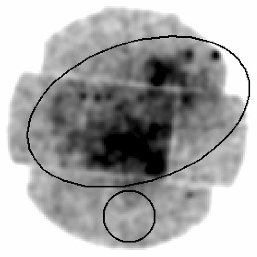
The EPIC-MOS2 image. The ellipse apertures (13.5 × 8.2 arcmin, major and minor axes, respectively) show the extension of the diffuse X-ray emission from SNR W51C. The circle (with radius 2.5 arcmin) shows the extraction region of the background spectrum.
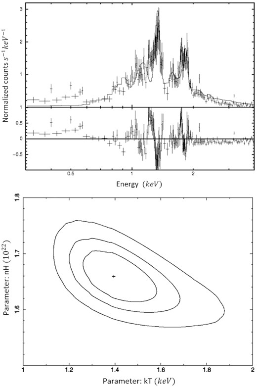
Top: Background-subtracted XMM–Newton EPIC spectra of SNR W51C. The solid lines show the best-fitting model. Bottom: Contours for 2D confidence levels of |$68{{\ \rm per\ cent}}$|, |$90{{\ \rm per\ cent}}$|, and |$99{{\ \rm per\ cent}}$| for internal, intermediate, and external contours, respectively.
To obtain the physical parameters of the hot gas, the spectrum was fitted using the xspec software (version 12.9, Arnaud 1996). The spectrum was fitted considering the thermal model vnei (Borkowski, Lyerly & Reynolds 2001) convolved with the tbabs absorption model (Wilms, Allen & McCray 2000). In this model we considered a galactic column density of NH = 1.6 × 1022 cm−2, and chemical abundances fixed to solar values (except for oxygen, 3.5 times the solar abundance). Our best-fitting model gives a reduced χ2 = 1.6. The best-fitting model is superposed to the background-subtracted EPIC spectrum in the top panel of Fig. 7. In the bottom panel of Fig. 7, we reproduce the plot of NH versus kT for the confidence levels of the χ2 fit. The best fit is labelled with a cross, while the contours correspond to |$68{{\ \rm per\ cent}}$|, |$90{{\ \rm per\ cent}}$|, and |$99{{\ \rm per\ cent}}$| confidence levels.
The best-fitting parameters in the [0.3–4.0] keV energy band are listed in Table 4, where kT is the gas temperature, Vs is the shock velocity given by Vs = (16kT/3μ)1/2 with μ = (14/11)mH (Weaver et al. 1977), |$t=\frac{2}{5}{R}/{V_\mathrm{s}}$| (where R is the linear radius of the RSN) is the age of the RSN, A is the normalization parameter, Lx is the intrinsic luminosity, fx is the intrinsic X-ray flux, ne, x is the electron density, and τ = ne, xtion is the ionization time-scale. The pressure and thermal energy are given by |$P_x=n_{e,x} kT$| and |$E_\mathrm{th}=\frac{3}{2}n_{e,x}VkT$|, respectively (where V is the volume of X-ray emission from the SNR). Finally, for Sedov SNRs the initial energy of the explosion is E0 = 1.4Eth. The values of these parameters are calculated, when needed, by considering a distance to the SNR of D = 4.1 ± 0.2 kpc (see Section 3.1.2).
7 NUMERICAL SIMULATIONS AND RESULTS
For modelling the SNR evolution we used a freely available python code (Leahy & Williams 2017). It includes a clumpy ISM model, the Sedov–Taylor model, and a free-expansion model (referred to as the ‘standard model’ in the python code) for the SNR. First, we determine the evolution of the SNR by employing the cloudy ISM model. To run the model, the SNR explosion input parameters are the following: age (in years), energy E0 (in units of |$10^{50}\, \rm erg$|), ejected mass Meject (in units of solar mass M⊙), and the power-law index describing the density stratification of the ejecta, i.e. ρ ∝ r−n. The ISM parameters are: density stratification ρISM ∝ r−s, temperature TISM, the cooling adjustment factor (1 for solar abundance), and the random speeds associated with the ISM turbulence σν (|$\rm km~\rm s^{-1}$|). For s = 0, the uniform density is specified by the ISM number density. The electron-to-ion temperature ratio is calculated as shown in Leahy & Williams (2017). The default values for the ISM abundance are solar (Grevesse & Sauval 1998). Output parameters for the blast-wave forward shock and reverse shock are the radius, velocity, temperature of electrons, and emission measure (if applicable), all given as a function of time, as well as several plots, including the forward shock radius versus time, forward shock velocity versus time, reverse shock radius versus time, reverse shock velocity versus time, and emission measure versus time. We refer the interested reader to the paper by Leahy & Williams (2017) for more details on the code.
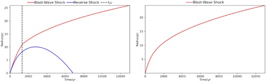
As W51C is an MM SNR (see Section 5), we apply the WL model. This model depends on two parameters: the cloud density parameter C = ρc/ρo, where ρc and ρo are the cloud and the intercloud densities, and the evaporation time-scale parameter τ* = tevap/t, where tevap is the evaporation time-scale of the SNR (see equation 6 of Slavin et al. 2017). The WL model reduces to one parameter C/τ* in the limits of C, τ* → ∞. To evaluate the case of SNR W51C, we used the one-parameter limit in the model. The package allows us to choose the ratio C/τ* among the values 0, 1, 2, or 4. In our model, we employed the value C/τ* = 4. The input and output parameters are displayed in Table 5. At the derived SNR age, the SNR size obtained from the model is 25.9 pc (see the left-hand panel of Fig. 8), and the blast-wave shock velocity is 750 km s−1. These values are comparable with R = 24 pc and Vs = 750 km s−1 that we reported in Table 4. The estimated electron temperature is significantly different, since the code gives a value of 5.4 × 10⁶ K, while we derived a temperature of ∼1.6 × 10⁷ K from our observations.
Left: selection of the output plot of radius versus time; this plot represents the size of the blast-wave shock (red) and of the reverse shock (blue) for the cloudy ISM model. Right: the same for the Sedov–Taylor model.
Numerical models (Leahy & Williams 2017).
| Cloudy ISM model | |
|---|---|
| Input parameters | Value |
| Age (yr) | 13 000 |
| Energy (|$\times 10^{50}\rm \,erg$|) | 8.4 |
| Ejected mass (M⊙) | 1.4 |
| Ejecta power-law index, n | 0 |
| CSM power-law index, s | 0 |
| Electron-to-ion temperature ratio Te/Ti | 0.34 |
| Cooling adjustment factor | 1.0 |
| ISM number density (|$\rm cm^{-3}$|) | 0.0126 |
| ISM turbulence/random speed (|$\,\rm km\,s^{-1}$|) | 7.0 |
| C/τ* | 4 |
| Output parameters | Value |
| Blast-wave shock electron temperature (K) | 5.457 × 10⁶ |
| Blast-wave shock radius (pc) | 25.94 |
| Blast-wave shock velocity (km s−1) | 750 |
| Sedov–Taylor model | |
| Input parameters | Value |
| Age (yr) | 13 000 |
| Energy (|$\times 10^{50}\rm \,erg$|) | 8.4 |
| ISM temperature (K) | 100 |
| Ejecta power-law index, n | 0 |
| CSM power-law index, s | 0 |
| Electron-to-ion temperature ratio Te/Ti | 0.67 |
| Cooling adjustment factor | 1.0 |
| ISM number density (|$\rm cm^{-3}$|) | 0.05 |
| ISM turbulence/random speed (|$\,\rm km\,s^{-1}$|) | 7.0 |
| Output parameters | Value |
| Blast-wave shock electron temperature (K) | 1.069 × 10⁷ |
| Blast-wave shock radius (pc) | 24.33 |
| Blast-wave shock velocity (km s−1) | 750.7 |
| Standard model | |
| Input parameters | Value |
| Age (yr) | 13 000 |
| Energy (|$\times 10^{50}\rm \,erg$|) | 8.4 |
| ISM temperature (K) | 100 |
| Ejected mass (M⊙) | 1.4 |
| Ejecta power-law index, n | 7 |
| CSM power-law index, s | 0 |
| Electron-to-ion temperature ratio Te/Ti | 0.67 |
| Cooling adjustment factor | 1.0 |
| ISM number density (|$\rm cm^{-3}$|) | 0.05 |
| ISM turbulence/random speed (km s−1) | 7.0 |
| Output parameters | Value |
| Blast-wave shock electron temperature (K) | 1.074 × 10⁷ |
| Blast-wave shock radius (pc) | 24.3 |
| Blast-wave shock velocity (km s−1) | 752.5 |
| Emission measure (|$\rm cm^{-3}$|) | 1 × 1058 |
For comparison, we employed the Sedov–Taylor model with the same set of parameters, except for an ISM number density of 0.05. The results obtained are: a radius of |$24.33 ~\rm pc$|, a blast-wave shock velocity of 750.7 km s−1, and a blast-wave shock electron temperature of 1.1 × 10⁷ K, in agreement with the observations. In the right-hand panel of Fig. 8 we show the blast-wave shock radius versus time.
To reproduce the emission measure parameter the ‘standard model’ is considered for the early evolution of the SNR (i.e. during the freely expanding phase). In this case, the input parameters are similar to the above models, but with an ejecta power-law index n = 7 and a power-law index s = 0. The left-hand panel of Fig. 9 shows the blast-wave radial position versus time. We obtained a radius of |$24.3 ~\rm pc$| at the current SNR age. The shock velocity is |$752.5 ~\rm km~s^{-1}$| and the electron temperature is |$1.1 \times 10^{7}~\rm K$|. These values are in agreement with those obtained in Table 4. The model predicts an emission measure of |$\sim 1\times 10^{58}~\rm cm^{-3}$|, while the one obtained above is |$\sim 0.5 \times 10^{58} ~\rm cm^{-3}$| (see the right-hand panel of Fig. 9). Table 5 shows the input and output parameters for the models described above.
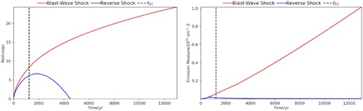
Left: selection of the output plot of radius versus time; this plot represents the size of the blast-wave shock (red) and of the reverse shock (blue) for the standard model. Right: selection of the output plot of emission measure versus time; this plot represents the behaviour of the emission measure along time.
8 DISCUSSION AND CONCLUSIONS
From the optical data we obtained the systemic velocity and derived the kinematic distance to SNR W51C. The derived distance is much shorter than other distance estimates and consequently the linear diameter is smaller than previous determinations. We also derived the velocity of the shock induced in the dense clouds immersed in the rarefied medium where the primary blast wave travels, as well as the density of the clouds.
In addition, we conducted a detailed study of SNR W51C in the Milky Way based on XMM–Newton data. We have generated X-ray images and spectra of this object and find that the SNR shows a central bright X-ray morphology due to thermal emission surrounded by a non-thermal radio-emitting shell; see Fig. 5. Therefore we confirm the classification of W51C as an MM SNR. Similar features were found in SNRs W44 (Jones, Smith & Angelini 1993), 3C 391 (Rho & Petre 1996), G272−3.2 (Harrus et al. 2001), and 0520−69.4 (Ramírez-Ballinas et al. 2020). Consequently, all of them are excluded from the group of SNRs whose centres are dominated by non-thermal emission, presumably due to a central pulsar.
The WL model was proposed to explain the mixed-morphology class of SNRs as being caused by the evaporation of dense clouds overrun by the blast wave. From the optical observations at [S ii], we estimate a cloud density ranging from 1.0–|$200 \rm ~ cm^{-3}$| whereas the electron density derived from X-ray observations, 0.1 cm−3, corresponds to the intercloud density. Assuming that the pressure of the hot gas is similar to the pressure in the clouds, we take |$n_\mathrm{cl}=3.0 ~\rm cm^{-3}$| and |$V_\mathrm{cl}=75 ~\rm km~s^{-1}$| for the cloud mean density and the induced shock velocity, respectively, so that the ram pressure of the shock, |$\sim 2.0\times 10^{-10} ~\rm dyn~cm^{-2}$|, is similar to the value of the thermal pressure derived from the X-ray emission, |$P_{x}\, \sim 2.2\times 10^{-10} ~\rm dyn~cm^{-2}$|. Thus, the hot X-ray-emitting gas acts as the piston for this blast wave. We also derive a C parameter with a value of C = 30. In Table 6 we present the values for the parameters used in the WL model. From table 3 of WL, it was possible to obtain the value of the emission-weighted temperature <T >. From this model we derived reasonable values for the parameters obtained from the observations presented in this work, as radius and velocity blast-wave shock.
Physical parameters of SNR W51C, derived from this work, used in the models from WL.
| Vs | 750 km s−1 |
| t | 13 000 yr |
| ncl | 3.0 cm−3 |
| Rcl | 1.0 pc |
| tevap | 30 000 yr |
| τ* | ∼2.3 |
| C | 30 |
| <T > | ∼4.0 × 10⁶ K |
| C/τ* | 13 |
| Vs | 750 km s−1 |
| t | 13 000 yr |
| ncl | 3.0 cm−3 |
| Rcl | 1.0 pc |
| tevap | 30 000 yr |
| τ* | ∼2.3 |
| C | 30 |
| <T > | ∼4.0 × 10⁶ K |
| C/τ* | 13 |
Running several models of Leahy & Williams (2017) based on a python code, we considered three possible cases: Sedov–Taylor, standard, and cloudy (WL models for MM SNRs) models. All of them reproduce the values derived from observations. However, the mixed morphology of SNR W51C is only reproduced by the cloudy model and consequently we adopt the values derived from that model. For the value of the emission measure, the right-hand panel of Fig. 9, we found a value of the order of the observed one.
In this work, we obtain a more typical value of the energy deposited in the ISM by the SN explosion than the ones given in previous works. This value makes unnecessary the possibility of having several SN explosions. The value for the energy that we obtain agrees with the one computed more recently by Leahy & Ranasinghe (2018). Also, the ram pressure is similar to the thermal pressure while in previous works the ram pressure was estimated to be two orders of magnitude higher than the thermal pressure
More observational studies and detailed modelling employing numerical simulations are needed to determine the origin and evolution of mixed-morphology SNRs like the one studied in this paper.
ACKNOWLEDGEMENTS
JR-I acknowledges financial support from TNM-SEP, DGAPA-PAPIIT (UNAM) grant IG100516. MR is grateful for financial support from DGAPA-PAPIIT (UNAM) IN109919 and CONACYT CY-253085 and CF-86367 grants.
DATA AVAILABILITY
The X-ray data underlying this article are available in an XMM–NewtonScience Archive search at http://nxsa.esac.esa.int/nxsa-web/#search with the name of the object SNR W51C and Obs. ID 0554690101 (ODF files). Optical data underlying this article will be shared on reasonable request to the corresponding author.
Footnotes
cigale, for CInematique de GALaxiEs, is a piece of specialized software used to analyse Fabry–Pérot interferometric data cubes. It was developed by Etienne Le Coarer at the Marseille Observatory and is optimized for the analysis of internal motions in nebulae.
iraf is distributed by the National Optical Astronomy Observatory, operated by the Association of Universities for Research in Astronomic, Inc., under cooperative agreement with the National Science Foundation.
