


ABSTRACT
The narrow-line Seyfert 1 galaxy |$\rm I\,\,Zwicky\, 1$| shows a unique and complex system of ionized gas in outflow, which consists of an ultra-fast wind and a two-component warm absorber. In the last two decades, XMM–Newton monitored the source multiple times enabling the study of the long-term variability of the various outflows. Plasma in photoionization equilibrium with the ionizing source responds and varies accordingly to any change of the ionizing luminosity. However, detailed modelling of the past Reflection Grating Spectrometer (RGS) data has shown no correlation between the plasma ionization state and the ionizing continuum, revealing a complex long-term variability of the multiphase warm absorber. Here, we present a new observation of |$\rm I\,\,Zwicky\, 1$| by XMM–Newton taken in early 2020 characterized by a lower X-ray flux state. The soft X-ray spectrum from the RGS reveals the two components of the warm absorber with log ξ ∼ −1.0 and log ξ ∼ 1.7. Comparing our results with the previous observations, the ionization state of the two absorbing gas components is continuously changing, following the same unpredictable behaviour. The new results strengthen the scenario in which the ionization state of the warm absorber is driven by the density of the gas rather than the ionizing luminosity. In particular, the presence of a radiation driven, inhomogeneous clumpy outflow may explain both the variability in ionization throughout the years and the line-locked N v system observed in the ultraviolet band. Finally, the EPIC-pn spectrum reveals an ultra-fast wind with an outflow velocity of ∼0.26c and ionization parameter of log ξ ∼ 3.8.
1 INTRODUCTION
A supermassive black hole with mass between MBH ∼ 106–1010 M⊙ and accreting material through an accretion disc is the core engine of an active galactic nucleus (AGN). Although the hearts of these powerful sources are the same, their phenomenology shows an extended variety based on several parameters such as line-of-sight angle and mass accretion rate (Giustini & Proga 2019). Around |$\sim 50\!-\!65{{\ \rm per\ cent}}$| of nearby, bright, AGN show narrow absorption lines in their ultraviolet (UV) and X-ray spectra (e.g. Costantini 2010; Kriss et al. 2012; Tombesi et al. 2013; Laha et al. 2014). The plethora of absorption edges and lines imprinted by several ions in the soft X-ray band (0.2–2 keV) are known as a warm absorber and often show higher ionization components compared to their UV counterparts (e.g. Reynolds & Fabian 1995; Costantini et al. 2007b; Mehdipour, Branduardi-Raymont & Page 2010; Behar et al. 2017).
These absorption lines, predominately from astronomically abundant metals (e.g. C, N, O, Ne, and Fe), are observed to be blueshifted with respect to the systemic redshift. This indicates that the gas is outflowing. The ionization state of the absorber is usually expressed by the ionization parameter, ξ, defined as ξ = Lion/nr2 where Lion is the ionizing luminosity, n is the density of the gas, and r is the distance from the ionizing source. In many AGN, the warm absorber is a multicomponent medium with a wide range in ionization parameter (ξ ∼ 0.1–1000 erg cm s−1), column density (NH = 1019–1023.5), and outflow velocity (vout ∼ 100–3000 km s−1) and is very rarely detected as a single component (e.g. Kaastra et al. 2002; Kaspi et al. 2002; Detmers et al. 2011; Laha et al. 2014; Silva, Uttley & Costantini 2016).
In spite of the extensive knowledge acquired through high-resolution X-ray spectroscopy with the gratings aboard Chandra and XMM–Newton, there are still pending questions regarding warm absorbers in AGN. For example, their relation with other kinds of outflows observed in AGN, such as ultra-fast outflows (UFOs; Tombesi et al. 2010; King & Pounds 2015) and obscurers (Kaastra et al. 2014), is still discussed among the scientific community. Furthermore, the spatial extent of the warm absorbers and their distance relative to the central black hole are difficult to determine. The spatial location of the outflows holds crucial information on the launching mechanism of warm absorbers and on the AGN feedback in the surrounding environment (e.g. Crenshaw & Kraemer 2012; Fabian 2012; Veilleux et al. 2020).
An approach to estimate the distance of the absorber to the central source is monitoring the response of the gas to changes in the ionizing continuum. The ionization state of the gas responds to any change of the ionizing luminosity on a time-scale that yields information regarding the density of the gas (Krolik & Kriss 1995; Nicastro et al. 1999) and its distance from the central source (through the definition of the ionization parameter). The time that an ionized gas needs to reach the photoionization equilibrium following a variation in the ionizing luminosity is known as equilibrium time-scale and it is inversely proportional to the density of the plasma. Low-density gases reach their equilibrium slowly and they can show a lag between the evolution of the ionization state and the illuminating radiation. Several attempts have been made to map the warm absorber distribution along the line of sight using long observations of both broad- (Mrk 509; Kaastra et al. 2012) and narrow-line Seyfert 1 (NGC 4051; Krongold et al. 2007). These complex studies indicate distances between 0.1 and 500 pc.
In a handful of AGN, outflows show a deviation from the expected behaviour in which their ionization state responds with a possible delay to variations in ionizing luminosity. For example, the ionization state of the warm absorber gas detected in MR 2251-178 and Mrk 335 does not correlate with the X-ray luminosity (Kaspi et al. 2004; Longinotti et al. 2013). In MR 2251-178, the absorbing material seems to respond instantly to the ionization variations only on short time-scales (∼weeks). The odd long-term variability of the warm absorber properties can be explained with a changing absorber consisting of material that enters and disappears from the line of sight on time-scales of several months. Mrk 335 shows, instead, a complex warm absorber system where only the high-ionization component correlates with the X-ray flux variability, unlike the low-ionization absorbers.
In this work, we study the uncanny behaviour of the warm absorber detected in I Zwicky 1 (hereafter |$\rm I\:Zw\, 1$|). The source is the prototype of a narrow-line Type I Seyfert galaxy.1 By virtue of its high optical nuclear luminosity and low redshift (z = 0.061169) |$\rm I\:Zw\, 1$| is also known as the closest quasar (Springob et al. 2005). It is both a bright (|$L_{\rm X,\, (0.3\!-\!10\ keV)} \sim 10^{44}\ \rm erg\ s^{-1}$|; Gallo et al. 2004) and variable X-ray source (Wilkins et al. 2017).
The soft X-ray spectrum of |$\rm I\:Zw\, 1$| reveals the presence of a two-component warm absorber that has been detected in all three previous XMM–Newton observations. The properties of these outflows and their long-term variability have already been studied by Costantini et al. (2007a) and Silva et al. (2018). Both works noticed that the ionization states of the low- and high-ionization components do not correlate with the ionizing luminosity. This behaviour is hard to explain and makes the warm absorber of |$\rm I\:Zw\, 1$| one of a kind. Based on their observations, Silva et al. (2018) proposed a phenomenological model consisting of a clumpy outflow where the two gas components are potentially part of the same outflowing cloud, only differing in density and degree of exposure to the central source.
The hard spectrum of |$\rm I\:Zw\, 1$| shows the presence of a UFO. Analysing in detail the iron K band of the archival XMM–Newton observations, Reeves & Braito (2019) reported evidence for a fast (∼c) wide-angle wind which is commonly seen in systems that accrete at close to the Eddington limit, such as |$\rm I\:Zw\, 1$| (Porquet et al. 2004). The UFO presence is detected in three out of four epochs, with an ionization parameter log ξ ∼ 4.9. In the 2005 observation, the absorption features are contaminated by a complex emission spectrum in the iron region. Adopting a radiative disc wind model, the fast outflow in |$\rm I\:Zw\, 1$| shows a mechanical power within |$5{-}15{{\ \rm per\ cent}}$| of Eddington, while its momentum rate is of the order of unity (Reeves & Braito 2019). Comparing with the upper limits placed by the IRAM observation of the CO emission on the energetics of the molecular gas (Cicone et al. 2014), Reeves & Braito (2019) concluded that the scenario of a powerful, large-scale, energy conserving wind in |$\rm I\:Zw\, 1$| can be ruled out. They suggested the presence of a low efficiency mechanism in transferring the kinetic energy of the inner wind to the large-scale molecular component.
In this work, we present the analysis of the latest high-resolution X-ray spectrum taken during the XMM–Newton observation of 2020. The recently acquired data and its reduction are presented in Section 2. We introduce the spectral energy distribution (SED) of |$\rm I\:Zw\, 1$| in Section 3. The broad-band modelling is essential to determine the ionization state of the outflows described in Section 4. The results and their implications are discussed and summarized in Sections 5 and 6, respectively.
The spectral analysis and modelling presented here are performed using the spex fitting package (Kaastra, Mewe & Nieuwenhuijzen 1996; Kaastra et al. 2020) version 3.06.01. All the spectra shown in this work are background subtracted and displayed in the observed frame. We use both the C-statistic (Cash 1979) and Bayesian data analysis (Bayes 1763) for spectral fitting and provide errors at 1σ confidence level. In our calculation, we adopted the cosmological parameters as default in spex: |$H_0=70\ \rm {km}\ \rm {s}^{-1}\ \rm {Mpc}^{-1}$|, ΩΛ = 0.70, and Ωm = 0.30. We assume proto-solar abundances of Lodders (2010) throughout this paper.
2 OBSERVATIONS AND DATA REDUCTION
|$\rm I\:Zw\, 1$| was observed by XMM–Newton (Jansen et al. 2001) for two consecutive orbits (revolution 3680 and 3681) on 2020 January 12 and January 13 as part of the study of the X-ray spectrum and variability of the source (Wilkins et al. 2021). The two observations with obsID 0851990101 and 0851990201 (hereafter, observation 101 and 201, respectively) have a total nominal exposure time of 145.1 ks (75.8 ks and 69.3 ks, respectively). The XMM–Newton data were processed using the Science Analysis System (SAS, version 20.0) and CALDB v4.9.4.
The Reflection Grating Spectrometer (RGS; den Herder et al. 2001) was used to study the absorption-line-rich soft X-ray spectrum of |$\rm I\:Zw\, 1$|. The RGS data were gathered in the Spectroscopy HER + SES mode. The data were processed using the rgsproc pipeline task; the data and the background were extracted using default selection regions. Furthermore, we filtered out time intervals with background count rates >0.2 count s−1 in CCD number 9. The background filtering led to a loss of about 14.6 ks. The total net exposure time is then 120.5 ks with an average source count rate of |$\rm 0.244\pm 0.002\ count\ s^{-1}$|. The data were used in the spectral range between 7 Å (E ∼ 1.8 keV) and 37 Å (E ∼ 0.34 keV) and they were binned using the optimized binning routine obin (Kaastra 2017) implemented in the spex fitting package. For the time-averaged spectral analysis, we merged the two data sets and combined RGS1 and RGS2 in one single OGIP file (Arnaud, George & Tennant 1992) using the rgscombine task.
For the SED modelling, we fitted spectra from XMM–Newton EPIC-pn and OM. The EPIC-pn instrument (Strüder et al. 2001) was operated in Small-Window mode with the Thin Filter. The data were processed using the epproc pipeline task. Periods of high-flaring background for EPIC-pn (exceeding 0.4 count s−1) were filtered out while applying the #XMMEA_EP filter. We extracted a single event (PATTERN= = 0), high-energy (PI>10000 && PI<12000) light curve from the event file of the entire chip to identify intervals of high-flaring background. The last 2.5 ks of the first orbit (obsid 0851990101) has been filtered out due to the contamination by particle background. The XMM–Newton EPIC-pn spectra were extracted from a circular region centred on the source with a radius of 30 arcsec. The background was extracted from a nearby source-free region of radius 30 arcsec on the same CCD as the source. The pileup was evaluated to be negligible using the task eppatplot. The single and double events were selected for the EPIC-pn (PATTERN< = 4). Instrumental response matrices were generated for the spectrum using the rmfgen and arfgen tasks. We applied the energy dependent correction by Fürst (2022) to align the EPIC-pn and NuSTAR spectral shape. In specific, we added the XRT3_XAREAEFF_0014.CCF to our calibration files and invoked it explicitly by running arfgen with the flag applyabsfluxcorr = yes. The fitted spectral range for EPIC-pn is 0.3-10 keV and for the analysis we grouped the data following the optimal binning algorithm presented by Kaastra & Bleeker (2016).
The Optical Monitor (OM; Mason et al. 2001) photometric filters were operated in the Science User Defined image/fast mode. In both observations, OM images were taken with the V, B, U, UVW1, and UVW2 filters, with an exposure time between 2.3 and 4.4 ks for each image. The OM images of |$\rm I\:Zw\, 1$| were processed with the omichain pipeline with the standard parameters. The filter count rates and errors were extracted from a region with an aperture of 12 arcsec and written into a single spectral file using the om2pha task.
|$\rm I\:Zw\, 1$| was also observed continuously by NuSTAR between 2020 January 11 and 16 (ObsID 60501030002) for a total net exposure time of 233 ks. We followed the standard procedure using nustardas v. 1.9.2 to reduce the observations. The event lists from each of the focal plane module (FPM) detectors were cleaned and calibrated using the nupipeline task. Following Wilkins et al. (2021), we extracted the source photons from a circular region, 30 arcsec in diameter, centred on the source. The smaller 30 arcsec region, suitable for sources that are faint above 10 keV, was selected over the larger 60 arcsec region to maximize the signal to background ratio in the observation of |$\rm I\:Zw\, 1$|. Source and background spectra together with their response matrices were extracted and generated using the nuproducts tool. In the spectral analysis, we fitted simultaneously the 10–50 keV energy band of the separate NuSTAR spectra obtained from the FPMA and FPMB detectors.
All the reduced files were converted from the OGIP FITS format to the spex format using the auxiliary trafo program of the spex package.
3 SPECTRAL ENERGY DISTRIBUTION
In this section, we present our modelling of the spectral components that form the observed SED of |$\rm I\:Zw\, 1$|. We jointly model the spectra of the two observations. We derive the intrinsic UV-X-ray continuum by modelling the UV reddening and X-ray absorption along our line of sight towards the nucleus of |$\rm I\:Zw\, 1$|. The final SED continuum model of the source is shown in Fig. 1.
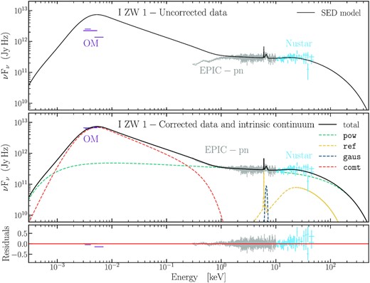
Average OM and EPIC-pn spectra of |$\rm I\:Zw\, 1$| from the XMM–Newton observation taken in 2020 together with the FPMA and FPMB spectra from the simultaneous NuSTAR observation. The data are displayed before (upper panel) and after (middle panel) corrections for the intrinsic extinction and for the Galactic reddening in the UV (Section 3.1) and in the X-rays (Section 3.2). The data correction includes the effects of absorption by the warm absorber and the UFO. The different components used in our SED modelling are overplotted. The fit residuals, (observed-model)/model, are displayed in the bottom panel.
3.1 UV continuum and reddening
To characterize the UV continuum emission, we used the U, UVW1, and UVW2 filters of OM. The B and V filters are not considered in this analysis because of the uncertainties about the host-galaxy contribution at those wavelengths. In our first approach to model the UV emission radiated by the disc, we adopted a disk blackbody component (dbb in spex) with the temperature coupled to the seed temperature of the Comptonization model (comt; Titarchuk 1994) used to characterize the soft X-ray excess (Section 3.2). The inclusion of the disc blackbody component does not improve the broad-band fit and comt alone is sufficient to get a good fit of the UV/soft X-ray band. Therefore, we decided to used only the comt model to fit the UV continuum emission. A similar modelling has been used to model the optical/UV/soft X-ray emission from NGC 5548 and NGC 7469 (Mehdipour et al. 2015, 2018).
The line-of-sight extinction affecting |$\rm I\:Zw\, 1$| is the sum of the intrinsic absorption, in the rest frame of |$\rm I\:Zw\, 1$|, and a component due to our Galaxy, in the observed frame. Assuming a Fitzpatrick (1999) reddening law with RV = 3.1, the foreground Milky Way reddening in our line of sight has a colour excess E(B − V) = 0.057 mag (Schlafly & Finkbeiner 2011). We applied an ebv component in spex to model this reddening, which incorporates the extinction curve of Cardelli, Clayton & Mathis (1989) including the update for near-UV given by O’Donnell (1994).
|$\rm I\:Zw\, 1$| exhibits a steep UV/optical continuum that suggests a large degree of intrinsic reddening (Laor et al. 1997). Using the flux measurements of the emission lines O i λ8446 and O i λ1304, Rudy et al. (2000) found an internal reddening of E(B − V) = 0.13 mag. We therefore correct the UV emission adding a second ebv component with the colour excess parameter fixed at this value.
3.2 X-ray continuum and absorption
To fit the time-averaged X-ray spectrum of |$\rm I\:Zw\, 1$|, we started with a power-law continuum (pow component in spex). The model mimics the Compton-up scattering of the disc photons in an optically thin, hot, corona. The high-energy exponential cut-off is fixed to 140 keV (Wilkins et al. 2022). A similar exponential cut-off has been applied to the power-law continuum in the low-energy band (Ecut = 13.6 eV) in order to prevent it from exceeding the maximum energy of the seed disc photons. We coupled the energy of the low cut-off with the temperature, Tseed of the seed photon of the Comptonization model. The photon index Γ of the intrinsic power law is 2.09 ± 0.01.
The soft X-ray continuum of |$\rm I\:Zw\, 1$| shows the presence of an excess above the power law (Gallo et al. 2004; Gliozzi & Williams 2020). Previous works fitted this excess using a broken power law with an energy break at 2 keV (Costantini et al. 2007b; Silva et al. 2018). The full modelling of the X-ray continuum of the 2020 observation of |$\rm I\:Zw\, 1$| has been presented in Wilkins et al. (2022). There the data showed a preference for a reflection model from an accretion disc with a radial ionization component that can well describe at the same time the soft X-ray excess, the Fe K α line and the Compton hump. Here, we aim at a simpler best fit, that models well the data while keeping a fast computational time of the photoionized code (see Section 4). We modelled the soft excess adopting the Comptonization model which fits well the emission fluxes in the U, UVW1, and UVW2 filters of OM, as shown before. In this interpretation of the soft excess, the seed disc photons are up-scattered in a warm, optically thick, corona to produce the extreme UV emission and the soft X-ray excess as its high-energy tail (e.g. Done et al. 2012; Kubota & Done 2018; Petrucci et al. 2018). In their modelling, Wilkins et al. (2022) noticed that the soft-excess can be equally well described by the emission from a warm corona that extends over the inner region of the accretion disc.
The parameters of the comt model are its normalization, seed photon temperature (Tseed), electron temperature (Te), and optical depth (τ) of the upscattering plasma. In order to avoid degeneracy between the plasma parameters of the X-ray soft excess and the UV emission, we fixed Tseed to a fiducial value of 1 eV and the optical depth to a value of 20. This limits the number of free parameters while still providing a good fit.
Subsequently, we added an X-ray reflection component (refl in spex) to take into account the reprocessing of the incident X-ray continuum, which is evident by the presence of the Fe K α line at 6.4 keV (Leighly 1999; Reeves & Turner 2000) and the Comptonization hump. The refl component computes the Compton-reflected continuum (Magdziarz & Zdziarski 1995) and the Fe K α line (Zycki, Done & Smith 1999). Similarly to the observed primary power law, the high-energy exponential cut-off of the incident power-law component has been set to 140 keV. We adopted solar metal abundances and we fixed the ionization parameter of refl to the lower limit of zero in order to produce a cold reflection component. Furthermore, we coupled the photon index Γ of the incident power law with the one of the primary power law and we fitted the reflection scale factor (s).
Previous observations of |$\rm I\:Zw\, 1$| have shown the presence of a broad ionized emission line in the iron K band centred at E = 7.0 keV (Gallo et al. 2007; Reeves & Braito 2019). Thus, we added a Gaussian profile (gaus in spex) to fit the emission from the partially ionized component. The normalization, the line energy (E0) and the full width at half-maximum of the Gaussian line have been computed.
In our SED modelling, we take into account the X-ray continuum and line absorption by the foreground diffuse interstellar medium in the Milky Way. We used the hot component in spex (de Plaa et al. 2004; Steenbrugge et al. 2005), which calculates the transmission of a plasma in collisional ionization equilibrium at a given temperature. To mimic the absorption by the intervening cold interstellar medium, we set the temperature to its minimum, kT = 0.008 eV (|$T\sim 100\,\, \rm K$|). The hydrogen column density was fixed to |$N_{\rm H}^{\rm MW} = 6.01\times 10^{20}\ \textrm {cm}^{-2}$| (Elvis, Lockman & Wilkes 1989; Willingale et al. 2013), which includes both the atomic and molecular hydrogen component.
Absorption by ionized AGN outflows significantly affects the X-ray spectral shape of |$\rm I\:Zw\, 1$| (Silva et al. 2018). In our spectral modelling, we take into account absorption by persistent outflows adopting the pion component in spex (Mehdipour, Kaastra & Kallman 2016). This model calculates the absorption spectrum from physical absorber parameters on the fly and therefore does not require any model grid preparation before data fitting. The warm-absorber models used here to fit the EPIC-pn data are based on a preliminary analysis of the RGS data set. We decided to neglect the high-ionization warm absorber component since it has a negligible impact on the spectral shape of the SED (see Section 4). The column density and the ionization parameter ξ (Krolik, McKee & Tarter 1981) of the low-ionization warm absorber and UFO were freed in order to improve the fit of the EPIC-pn data.
The best-fitting parameters of the power-law component (pow), warm Comptonization component (comt), the X-ray reflection component (refl), the Gaussian component (gaus) for the blend of H- and He-like Fe K α lines are provided in Table 1. The best fit to the data is shown in Fig. 1.
Best-value free parameters of the SED model (pow+comt+refl + gaus)*red*pion*ebvHG*ebvMW*hotMW.
| Parameter | Value | Units |
|---|---|---|
| Norm/pow | 1.95 ± 0.02 | |$\rm 10^{52}\ ph\ s^{-1}\ keV^{-1}$| |
| Γ/pow | 2.09 ± 0.01 | |
| Norm/comt | 1.25 ± 0.02 | |$\rm 10^{57}\ ph\ s^{-1}\ keV^{-1}$| |
| |$\rm t_1$|/comt | 0.12 ± 0.01 | |$\rm keV$| |
| Scal/refl | 0.43 ± 0.08 | |
| Norm/gaus | 6 ± 1 | |$\rm 10^{49}\ ph\ s^{-1}$| |
| E0/gaus | 7.07 ± 0.06 | |$\rm keV$| |
| FWHM/gaus | 0.6 ± 0.1 | |$\rm keV$| |
| F0.2 − 2 keV | 4.76 ± 0.01 | |$10^{-12}\ {\rm {erg\ cm}^{-2}\ \rm {s}^{-1}}$| |
| F2 − 10 keV | 4.73 ± 0.02 | |$10^{-12}\ {\rm {erg\ cm}^{-2}\ \rm {s}^{-1}}$| |
| Cstat/dof | 993/902 |
4 OUTFLOWS
We present here the AGN wind and its long-term variability through photoionization modelling and XMM–Newton RGS spectroscopy. For the spectral fitting of the absorption lines detected in the soft X-ray band, we used multiple pion components with elemental abundances fixed to the proto-solar values.
4.1 Time-averaged spectrum
To characterize the nuclear ionized outflows of |$\rm I\:Zw\, 1$|, we adopted the photoionization continuum presented in Section 3.2 and we analysed in detail the time-averaged RGS and EPIC-pn spectra of |$\rm I\:Zw\, 1$|. In Fig. 2, we show the residuals obtained fitting the data only with a galactic absorbed continuum model. In the energy band covered, there are several visible absorption features that are the typical signatures of intervening ionized absorbers. First, we added a pion component to account for the photoionization features impressed by the warm absorber. Given an SED the model computes both the photoionization solution and the transmitted spectrum of a plasma in photoionization equilibrium. The derived shape of the SED can indeed significantly influence the structure and thermal stability of the AGN outflows (see e.g. Chakravorty et al. 2012). The parameters of interest of the pion component are the hydrogen column density (NH), ionization parameter (usually expressed in logarithmic scale, log ξ), turbulence velocity (vturb), and outflow velocity (vout) of the ionized outflow.

Residuals of the RGS and EPIC-pn spectra (in black and blue, respectively) obtained fitting the 2020 XMM–Newton observation without any outflow component. We modified the x-scale in order to show clearly the residuals in both instruments. The dashed vertical line indicates where the scale changes. The residuals are defined as (data-model)/error.
We observed a warm absorber component with an ionization parameter log ξ = −1.0 ± 0.1 and column density |$N_{\mathrm{H}} = (9\pm 1)\times 10^{20}\rm \ cm^{-2}$|. Both outflow velocity (|$v_{\rm {out}} = -1750 \pm 100\rm \ km\ s^{-1}$|) and turbulence velocity (|$v_{\rm {turb}} = 110 \pm 30\rm \ km\ s^{-1}$|) of this low-ionization component (LIC, hereafter) are comparable with the lower ionization outflow observed in earlier data sets (Costantini et al. 2007b; Silva et al. 2018). To investigate the multiphase nature of the warm absorber, we added another pion component to our spectral model looking for the higher ionization warm absorber detected in earlier observations (e.g. Silva et al. 2018). We found an outflowing plasma with an ionization parameter of log ξ = 1.7 ± 0.2, column density |$N_{\mathrm{H}} = (1.0\pm 0.6)\times 10^{20}\rm \ cm^{-2}$| and outflow velocity |$v_{\rm out} = -2150^{+200}_{-250}\rm \ km\ s^{-1}$|. However, the statistical significance of the high-ionization component (HIC, hereafter) is low; the C improves by ΔCstat = 11 for 3 free parameters.
We also tested the presence of a UFO component. The time-averaged spectral analysis of the 2020 XMM–Newton observation reveals the presence of a UFO with hydrogen column density |$N_{\mathrm{H}} = (2_{-1}^{+3})\times 10^{22}\rm \ cm^{-2}$|, outflow velocity |$v_{\rm {out}} = -77\,100 \pm 400\rm \ km\ s^{-1}$| (∼0.26c) and ionization parameter |$\log \xi = 3.80_{-0.04}^{+0.11}$|. A UFO-like feature was already detected by (Wilkins et al. 2022). For this fast wind, the turbulence velocity was set to its default value of 100 km s−1. Adding this component to the broad model the statistic improves by ΔCstat = 45 for 3 free parameters. We did not detect any strong absorption feature in the iron K band. The transmitted spectrum of this fast outflow mainly improves the fit at lower energies, between 1 and 4 keV where multiple transitions by Si, S, and Fe are located.
We found a lower ionization parameter with respect to the previous work by Reeves & Braito (2019) which obtained a |$\log \xi = 4.91_{-0.13}^{+0.37}$|. This large discrepancy cannot be explained by only considering the discrepancy between different photoionization models and SED modelling. It might suggest instead that the ionization state of the UFO varies over year-long time-scales contrary to what has been observed in the previous XMM–Newton epochs (Reeves & Braito 2019).
When defining the relation between the different components inside spex, we ordered the ionized absorber components following the criterion that the higher ionization outflows are located closer to the central source shielding the lower ionization ones from the ionizing luminosity. Thus, each outflow component (UFO and warm absorbers) sees a different ionizing continuum. All the best-fitting parameter values of our modelling are listed in Table 2. We sorted the pion component by their significance. The best fit of the RGS and the EPIC-pn spectra are shown separately for clarity in Figs 3 and 4, respectively. For each ionized absorber, we also display the single transmittance spectral model which quantifies the respective contribution to absorption.
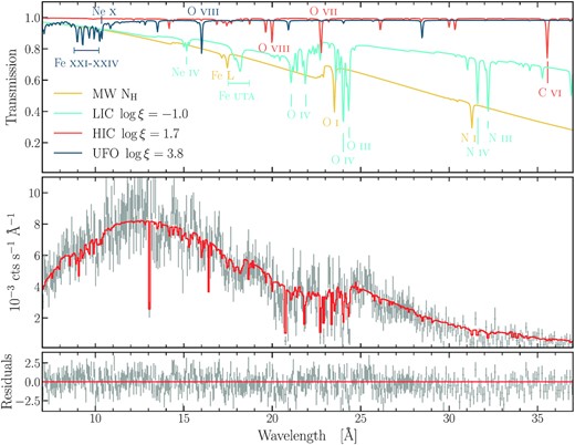
Combined RGS observations of |$\rm I\:Zw\, 1$| taken in 2020. Upper panel: transmission spectra of the detected warm absorbers (light-blue and red line), UFO (dark blue), and foreground neutral Galactic interstellar medium (yellow line). We labelled the strongest absorption features of the models. Middle panel: best fit of the RGS spectra of |$\rm I\:Zw\, 1$|. The spectrum has been binned for clarity of presentation. Lower panel: residuals of the best fit, defined as |$\rm (data-model)/error$|.

Combined PN observations of |$\rm I\:Zw\, 1$| taken in 2020. Upper panel: transmission spectra of the detected warm absorbers (light-blue and red line) and UFO (dark blue). The foreground Galactic neutral absorption is also shown (yellow line). We labelled the strongest absorption features of the models. Middle panel: best fit of the PN spectra of |$\rm I\:Zw\, 1$|. The spectrum has been binned using optimised binning (Kaastra 2017). Lower panel: residuals of the best fit, defined as |$\rm (data-model)/error$|.
Best-fitting parameters of the warm absorber components of |$\rm I\:Zw\, 1$| in the 2020 time-averaged spectrum inferred with a standard C-statistic analysis (on the left) and Bayesian framework (on the right).
| NH | log ξ | vturb | vout | C-stat/dof | NH | log ξ | vout | log Z | |
|---|---|---|---|---|---|---|---|---|---|
| |$10^{20}\ \rm cm^{-2}$| | |$\rm erg\ cm\ s^{-1}$| | |$\rm km\ s^{-1}$| | |$\rm km\ s^{-1}$| | |$10^{20}\ \rm cm^{-2}$| | |$\rm erg\ cm\ s^{-1}$| | |$\rm km\ s^{-1}$| | |||
| Single warm absorber component | |||||||||
| LIC | |$7.7_{-0.5}^{+0.8}$| | −1.0 ± 0.1 | |$110_{-25}^{+33}$| | −1750 ± 100 | 3218/2433 | 9.4 ± 0.6 | −1.2 ± 0.1 | −1750 ± 100 | −6.6 |
| Single warm absorber component + UFO | |||||||||
| LIC | 9.0 ± 0.7 | −1.0 ± 0.1 | |$90_{-20}^{+40}$| | −1750 ± 100 | 3173/2430 | 10.0 ± 0.5 | −1.2 ± 0.1 | −1750 ± 100 | 0.0 |
| UFO | |$200_{-100}^{+300}$| | 3.8 ± 0.1 | 100† | −77 100 ± 400 | 200 ± 50 | 3.8 ± 0.1 | −77 000 ± 3000 | ||
| Two warm absorber components + UFO | |||||||||
| LIC | 9 ± 1 | −1.0 ± 0.1 | 110 ± 30 | −1750 ± 100 | 3162/2427 | 9.4 ± 0.5 | −1.2 ± 0.1 | −1750 ± 100 | −0.3 |
| HIC | 1.0 ± 0.6 | 1.7 ± 0.2 | 100† | |$-2150_{-250}^{+200}$| | 0.9 ± 0.3 | 1.8 ± 0.3 | −2150 ± 350 | ||
| UFO | |$200_{-100}^{+300}$| | |$3.80_{-0.04}^{+0.11}$| | 100† | −77 100 ± 400 | 200 ± 50 | 3.8 ± 0.1 | −77 000 ± 3000 | ||
Note. †The dispersion velocity has been fixed to the default value of 100 km s−1.
In parallel to the X-ray spectral analysis based on the C-statistic, we characterized the AGN ionized outflows with Bayesian parameter inference. The Bayesian approach has the advantage of exploring the entire parameter space identifying sub-volumes that constitute the bulk of the probability. We used the MultiNest algorithm (v3.10 Feroz; Hobson & Bridges 2009; Feroz et al. 2013) and we adapted the PyMultiNest and Bayesian X-ray Analysis, BXA, packages (Buchner et al. 2014) to the spex fitting code (Rogantini et al. 2021).
To test the significance of each warm absorber component, we run the analysis twice starting with a model with one single pion component and then adding a second component. In both models, we included an additional photoionization model to characterize the UFO. In order to minimize the number of free parameters and to speed up the analysis we fixed the turbulence velocity to its default value (|$100\ \rm km \ s^{-1}$|). We assumed uninformative priors for the column density, ionization parameter, and outflow velocity of each pion model. The corner plot of the final parameter distributions is displayed in Fig. A1 for the model with three pion components.
In addition, the Bayesian framework provides a robust model comparison based on the Bayesian evidence, Z, which represents the posterior probability of the model given the data (see Buchner et al. 2014, and references therein for a detailed explanation). This method does not make any assumptions about the parameter space or the data. We computed and compared the evidence of the two models (with and without the HIC) adopting the scale of Jeffreys (1961) that excludes models with a Bayes factor of 30 (a difference of 1.5 in log Z). Both models show a comparable significance and there is not any strong evidence against the second warm absorber component. We cannot therefore exclude the presence of the HIC. The parameter values inferred with the Bayesian approach are listed on the right side of Table 2 together with the Bayesian evidence of each model.
4.2 Time resolved spectroscopy
The EPIC-pn light curve of |$\rm I\:Zw\, 1$| shown in Fig. 5 exhibits a double peak during the first observation (see Wilkins et al. 2021) likely due to the intrinsic variability of the corona. This rapid change in flux represents a good probe to test if any outflow responds to the ionizing luminosity on time-scale of hours. Thus, we performed a time-resolved spectral analysis of the |$\rm I\:Zw\, 1$| observations taken in 2020.

EPIC-pn light curve of the |$\rm I\:Zw\, 1$| observations taken 2020. We overplot the light curve extracted in different energy ranges. |$\rm {Time} = 0$| corresponds to the starting time of the first observation (MJD = 58860.94956941). The dashed vertical lines delimit the extraction sectors used for the time-resolved spectral analysis.
We split each observation into two sectors, obtaining in total 4 sectors of ∼40 ks each. Both peaks are included in the second sector (see Section 2). In order to consider variation of the ionizing luminosity in our spectral modelling of the outflow, we computed the SED for each sector following the same method presented in Section 3. We assumed that the UV flux does not change on this short time-scale. Wilkins et al. (2022) observed a variability at the 4 per cent level in the UV light curve of OM. Therefore, we simultaneously characterize the RGS and EPIC-pn spectra for each sub-epoch to study the short-term evolution of the ionized outflows of |$\rm I\:Zw\, 1$|.
To fit the spectra, we have taken advantage of the constraints we obtained from the fit of the time-averaged spectrum using the same continuum as a starting point. We kept fixed the parameters of the HIC to the values from Table 2 because of its low significance and we investigated any evolution of the column density, ionization parameter, and outflow velocity for the LIC and the UFO.
In Fig. 6, we show the results of our time-resolved spectroscopy of the 2020 observation of |$\rm I\:Zw\, 1$|. We compare the evolution of the ionization state, column density, and outflow velocity of the LIC and UFO with the |$0.3{-}10\, \rm {keV}$| light curve (top-panel).
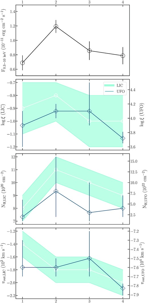
Time-resolved spectroscopy analysis. In the top panel, we show the 0.3–10 keV flux for each sector. In the second, third, and fourth panels, we plot, respectively, the evolution of the ionization parameter, column density, and outflow velocity for both the low-ionized warm absorber (shaded light blue, left y-axis) and the UFO (dark blue, right y-axis.).
The ionization parameter of the UFO (blue line in the second panel) drops between the second (log ξ = 4.1 ± 0.1) and the last sector (log ξ = 3.72 ± 0.08). Because of the large best-fitting uncertainties obtained in the other sectors it is difficult to determine if there is a correlation or a time delay between the light curve and the ionization parameter for the considered time-scales. However, we noticed an increase of significance of the UFO component in the last sector, where the uncertainty of both the column density and the ionization parameter is notably smaller. This is corroborated by the grid searches that we computed for each sector and displayed in Fig. B1 in Appendix B. The NH and ξ of the UFO in the fourth sector are better constrained and the their contour plot covers a smaller area in the parameter space. In this sector, the UFO component improves the overall fit by ΔCstat = 50.
Across the different time intervals, the outflow velocity of the UFO seems to follow an evolution similar to the ionization state whereas the column density varies within the uncertainties. The LIC instead shows a column density evolution suggesting that a larger amount of material is found along the line of sight in correspondence with the highest flux. Regarding the ionization state of the gas, the LIC does not vary within the errors whereas its outflow velocity increases between the first and second sectors.
The best-fitting parameters for each sector are listed in Table 3. Overall, the low signal-to-noise prevents an accurate time-resolved spectroscopy of the outflows. The present statistics together with the time gap between the two observations make it difficult to understand whether the outflows are in equilibrium with the ionizing radiation or if the column density and outflow velocity vary on the considered time-scales.
Time-resolved spectroscopy: best-parameters of the outflows.
| LIC | UFO | ||||||
|---|---|---|---|---|---|---|---|
| NH | log ξ | vout | NH | log ξ | vout | C-stat/dof | |
| |$10^{20}\ \rm cm^{-2}$| | |$\rm erg\ cm\ s^{-1}$| | |$\rm km\ s^{-1}$| | |$10^{22}\ \rm cm^{-2}$| | |$\rm erg\ cm\ s^{-1}$| | |$\rm km\ s^{-1}$| | ||
| Sec 1 | 8 ± 1 | −0.9 ± 0.2 | −1400 ± 200 | |$2^{+4}_{-1}$| | |$3.9^{+0.2}_{-0.3}$| | |$-76\,000^{+3000}_{-1000}$| | 849/684 |
| Sec 2 | 11 ± 1 | |$-0.8_{+0.1}^{-0.2}$| | −1800 ± 200 | |$8^{+8}_{-6}$| | 4.1 ± 0.1 | −76 000 ± 1000 | 772/689 |
| Sec 3 | 10 ± 1 | −1.0 ± 0.2 | −1800 ± 200 | |$3^{+7}_{-2}$| | |$4.1^{+0.4}_{-0.2}$| | |$-75\,000^{+3000}_{-2000}$| | 800/686 |
| Sec 4 | 9 ± 1 | −1.0 ± 0.2 | −2000 ± 200 | |$4^{+3}_{-2}$| | |$3.72^{+0.09}_{-0.07}$| | |$-78\,300^{+500}_{-800}$| | 902/684 |
5 DISCUSSION
The recent RGS data sets taken in early 2020 show the presence of a two-zone warm absorber in the soft X-ray band of |$\rm I\:Zw\, 1$|. The results, presented in the previous sections, become particularly interesting when compared with the outflow properties observed in the previous epochs. Here, we discuss the long-term variability of the warm absorbers in |$\rm I\:Zw\, 1$|, their origin and energetics. In addition, the EPIC-pn spectra of the source endorse the presence of a persistent UFO already detected in early epochs. The light curve of the present data sets provides a test bench to investigate any short-term response of the gas to the ionizing luminosity. In this section, we will discuss our attempt to carry out a detailed time-resolved spectroscopy study.
5.1 Variability of the warm absorbers
During its 23 yr long lifetime, XMM–Newton observed |$\rm I\:Zw\, 1$| multiple times. The soft X-ray spectra retrieved in earlier epochs, 2002, 2005, and 2015, all required a two-component warm absorber, consisting of a low-ionization and a high-ionization plasma that are not in pressure equilibrium (Costantini et al. 2007b; Silva et al. 2018). The 2020 data set presented here shows the same phenomenology.
In Fig. 7, we plot the variability of the hydrogen column density of the two-component warm absorber through the years. In the last observation, the HIC (in red) shows a significantly low column density, which compromises its detection significance, with respect to the previous epochs. The NH of the LIC (in blue) varies substantially among the XMM–Newton observations, dropping by at least a factor of five between 2002 and 2015 and increasing by a factor of three between 2015 and 2020. In contrast, the outflow velocity of both components has been constant over the past two decades (see Fig. 8). A similar velocity for the LIC was observed even at earlier epochs through UV spectroscopy (|$v_{\rm out} \sim 1870\rm \ km\ s^{-1}$|; Laor et al. 1997). Due to the shorter exposure time, it has not been possible to constrain the flow velocity for the HIC in the first two epochs (Costantini et al. 2007b).

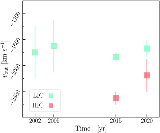
Long-term variability of the outflow velocity of the two warm absorbers. The velocities of the epoch 2002 and 2005 are taken from Costantini et al. (2007b) whereas the 2015 velocities are from Silva et al. (2018). The outflow velocity of 2002 and 2005 are not plotted here since only upper limits were obtained in these two epochs.
The ionization state of both outflowing plasmas exhibits a peculiar long-term variability. In Fig. 9, we plot the X-ray luminosity for all four epochs versus the ionization state of the two warm absorbers. The X-ray luminosity alone represents a good diagnostic for the ionizing luminosity since the ions in the X-ray band are more sensitive to high-energy photons (Netzer et al. 2003). We also display how the ionization state of the LIC and HIC relates with the UV flux observed by OM in the UVW2 filter, which is the only filter in common among all the observations. In both panels, the ionization balance of two warm absorbers manifests either a complex or a stochastic time-dependent behaviour. Possible explanations to this non-standard evolution of the outflow ionization states are given in Section 5.2.

Long-term variability of the ionization parameters as a function of the X-ray luminosity (on the left) and UV emission (on the right). Left-hand panel: We updated fig. 5 of Silva et al. (2018) adding the last observation (at the time of writing) taken in 2020. Throughout the year the ionization states of the outflowing plasma do not change accordingly with the X-ray ionizing luminosity. Right-hand panel: for comparison purpose we plot the variability of the ionization parameters as a function of UV emission observed with the UVW2 filter. We highlight the results of the present observation with the vertical yellow area whereas the results of previous epochs are indicated with the vertical grey bands.
The ionization states of the warm absorbers detected in |$\rm I\:Zw\, 1$| clearly do not vary directly following the ionizing luminosity. However, the ionization state of the two components seems to vary in the same way through the different XMM–Newton epochs. In the first three observations, we observed an apparent anticorrelation between their ionization parameters and the X-ray luminosity. In the 2020 observation, the LIC and HIC ionization parameters and the X-ray luminosity drop close to their historical minimum in qualitative agreement with a standard scenario where a plasma in photoionization equilibrium responds to the ionizing flux.
Finally, based on the model proposed by Silva et al. (2018) and summarized in the following section we can assume that the distance of the warm absorber does not change across the epochs. Thus, we can roughly estimate the absorber density variations using the definition of the ionization parameter. For this reason, it has been necessary to compute the ionizing luminosity between 1 and 1000 Ryd for each epoch.
This quantity is not available for the previous observations. For each XMM–Newton data set, we uniformly characterized the accessible OM filters and the EPIC-pn spectrum using the SED model adopted in this work. The best-fitting SED from each epoch is compared in Fig. 10. Both the shape and the normalization of the SED of |$\rm I\:Zw\, 1$| clearly vary over year-long time-scales. The densities of the LIC and HIC, shown in Fig. 11, normalized for their value observed in 2002, seem to vary consistently on time-scales of years. Starting from the density variation we can infer the changes in the warm absorber thickness, Δr, through the relation NH = f · n · Δr and assuming that the filling factor, f, remains constant over time. The right-hand panel of Fig. 11 demonstrates that the thickness of the two warm absorber components seems to follow the same evolution within each other over the epochs.

Comparison of the SED of |$\rm I\:Zw\, 1$| based on the OM and EPIC-pn data.

Left-hand panel: Variation of volume density of the warm absorbers, nH, assuming the same distance. We normalized for the initial density. Right-hand panel: Variation of the thickness, Δr of the warm absorber through the different RGS epochs. We normalized for the observation taken in 2002.
The different ionization measurements in this work and the previous literature cannot be explained by a distinct SED modelling. Costantini et al. (2007a) and Silva et al. (2016) used indeed a pure phenomenological model fitting the UV and X-ray data by means of a piecewise power law. Using the SEDs showed in Fig. 10, we reanalysed the properties of the outflows detected in the older observations. There are no significant differences between our best values and the ones from the literature. The column density and ionization parameter of LIC always vary within the uncertainties whereas we found slightly higher ξ for the HIC (between 1 and 2.5σ). The different SED modellings have a negligible effect on our results about the long-term variability of the ionized absorbers.
We have also studied the short-term variability of the warm absorbers dividing the light curve in four sectors. Due to its low-significance, we fixed the HIC parameters and investigated the short-term behaviour of the LIC. If the LIC were in photoionization equilibrium with the ionizing luminosity we would expect to see the ionization state of the LIC increasing by a factor of ∼2 (0.3 dex) between the first and second sector following the change in flux. However, the large uncertainties on the inferred ionization parameter values make it impossible to detect significantly if the gas responds or not to the ionizing luminosity. Instead, both the column density and the outflow velocity of the LIC seem to change on time-scale of hours. There is a tentative evidence that X-ray flares are accompanied by an increase of material and velocity. A similar short-term behaviour was observed by Silva et al. (2018) for the HIC during the X-ray peak present in the observation taken in 2015.
During the high-state observed in sector 2, the count rate is comparable with the count rate recorded in some segments of the 2015 observation (in particular with the segment 2 in table 3 of Silva et al. 2018). The ionization parameters of LIC in sector 2 of 2020 (|$\log \xi = -0.8_{+0.1}^{-0.2}$|) and in segment 2 of 2015 (log ξ = −0.4 ± 0.2) appear consistent within 2σ. However, both values are affected by large uncertainties that impede us from drawing any robust statement.
5.2 Origin of the warm absorber in I Zw 1
The preliminary analysis of the HST/COS data of |$\rm I\:Zw\, 1$| taken during the multiwavelength campaign of 2015 reveals the line-locking of the N v λ1239, 1243 doublet lines (Silva et al. 2018). This warm absorber observed in the UV is believed to be the counterpart of the LIC in the X-rays (Costantini et al. 2007b). The locked N v lines would provide important hints about the acceleration mechanism of the LIC. Line-locking systems are usually believed to be a signature of outflows driven by radiation forces. Lines formed in different outflow clumps can become locked at the doublet line separation due to shadowing effects in radiatively driven outflows. Under certain circumstances, clouds closer to the origin of the outflows can shield clouds further out resulting in a synchronizing of the outflow velocity (Milne 1926; Scargle 1973; Braun & Milgrom 1989). Whereas the C iv line-locking feature is largely visible in both broad absorption quasars (BALs) and non-BALs quasars, the line-locking feature from N v is often non-detected (Bowler et al. 2014; Mas-Ribas & Mauland 2019). Therefore, the outflows of |$\rm I\:Zw\, 1$| might represent a peculiar system both in the UV and in the X-rays. The UV data will be presented in detail by our team in a future paper.
To explain the non-trivial behaviour of the ionization states of the absorbers as a function of luminosity, Silva et al. (2018) proposed a phenomenological model in which different clumps, with different density, cross the observer’s line of sight at different epochs. In this configuration, the ionization state is driven by the different densities of the clouds and not by the ionizing luminosity (Dyda & Proga 2018). In this respect, a clumpy outflow can naturally explain the changes in opacity of the warm absorbers observed in the different data sets.
Silva et al. (2018) suggested that the two-phase warm absorber arises from the same clump, with the HIC facing the central source, since their ionization parameters followed the same evolution. Our results from the time-averaged analysis of the 2020 XMM–Newton campaign support the clumpy configuration suggested by Silva et al. (2018). The fact that the outflow velocity of both warm absorber components did not change indicates that we are staring at the same ejection phenomenon throughout all the epochs. The slightly higher velocity of the HIC agrees with the standard radiatively driven wind model (Proga, Stone & Drew 1998; Waters, Proga & Dannen 2021) where the less-dense, higher velocity, stream is confined at the more distant side of a denser, colder, and slower outflow. The connection between the two components would also provide a natural explanation for the similar evolution of the density and thickness of the two components over the last 20 yr (Fig. 11).
As an alternative, the odd behaviour of the warm absorber in |$\rm I\:Zw\, 1$| could be explained by a scenario in which the outflowing absorbing gas is in persistent non-equilibrium with the ionizing source. In general, for a gas in photoionization equilibrium, the plasma responds instantaneously to a variable source luminosity becoming more ionized as the flux increases and recombining when the flux of the source drops. In the presence of a low-density gas, its response to the change in luminosity may either be delayed or negligible (Nicastro et al. 1999; Kaastra et al. 2012; Silva et al. 2016). Unfortunately, the history of the ionizing luminosity before each considered epoch is not known. No RXTE, Swift, NICER monitoring has ever been planned before the XMM–Newton epochs. Therefore, it is not possible to infer the typical time delay of the warm absorbers with a time-dependent photoionization modelling (Rogantini et al., submitted).
5.3 Ultra-fast outflow detection
The coexistence of warm absorbers and UFOs has been observed along the line of sight of multiple AGN. Tombesi et al. (2013) noted that 70 per cent of the Seyfert 1 galaxies in their sample with a detected UFO also show a warm absorber. |$\rm I\:Zw\, 1$| can be added to this subset of sources since already earlier XMM–Newton/EPIC-pn observations reveal the presence of such a fast wind (Reeves & Braito 2019). In the observation of 2015, the presence of a blueshifted absorption line at 9 keV suggests the presence of an accretion disc wind with an outflow velocity of ∼0.26c and ionization parameter log ξ = 4.9. Analysing the broad and P-Cygni iron K profile of the 2002, 2005, and 2015 observations, Reeves & Braito (2019) did not observe any significant long-term variability in those data sets though wind parameters estimated in the earlier epochs are affected by large uncertainties.
In our fit, the outflow velocity of the gas is unchanged with respect to previous epochs (|$v_{\rm out} = -77\,100\pm 400\ \rm km\,s^{-1}$|; ∼0.26c), while its ionization state is significantly lower (|$\log \xi = 3.80_{-0.04}^{0.11}$|). The best-fitting value of the ionization parameter is driven by the shape and the absorption features of iron, silicon, and sulfur at lower energies (in Figs 3 and 4). In the Fe K band, we did not detect any statistically significant absorption feature at 9 keV. Instead, the best-fitting model highlights the presence of an absorption line at a lower energy of 8 keV.
Similarly to the warm absorber, the outflow velocity of the UFO does not show long-term variability. We are likely observing at the same wind which has changed its ionization state between 2015 and 2020. Between the two epochs the ionizing luminosity dropped by a factor of ∼2; thus, it cannot fully motivate the one-order of magnitude decrease observed for the ionization parameter. A clumpy system where the ionization state is density driven could explain the large variation of the ionization parameter. In the 2015 observation, Reeves & Braito (2019) found a discrepancy between the ionizing luminosity predicted by their radiative disc wind modelling and versus the observed luminosity. An inhomogeneous and clumpy wind represents one of the explanations proposed by the authors to explain the discrepancy without requiring the intrinsic X-ray luminosity to be suppressed. Finally, the probability distribution of the wind outflow velocity computed in the Bayesian data analysis shows multiple peaks (see Fig. A1). This also might suggest the presence of a system with a complex outflow velocity distribution rather than a single speed wind. The low signal-to-noise ratio prevents us from investigating it further.
A short-term variability of the ionization state of the UFO is also observed. During the X-ray flares the wind shows a higher ionization state with respect to the second data set (in particular sector 4) that comes after the flaring period. These results are suggestive that the ionization state of the UFO responds to the flaring in the X-ray emission on short time-scales. Wilkins et al. (2022) also noticed a variable highly ionized absorption line in the Fe K band for the same data sets using a Gaussian line scanning (see Pinto, Middleton & Fabian 2016). In the 2015 observation, the opacity of the wind appears to be anticorrelated with the X-ray flux on short time-scales (Reeves & Braito 2019). Here, the opacity change could either be due to a response in ionization of the wind, as we might observe in the present observation, or via modest variation of the wind column density.
5.4 Outflow energetics in I Zw 1
In contrast to other sources, |$\rm I\:Zw\, 1$| has proved to host a peculiar warm absorber system, whose geometry may differ from a classical conical structure where the AGN outflows are stratified according to ionization and distance. Therefore, directly connecting the UFO and the warm absorber as layers of the same structure (e.g. Tombesi et al. 2013) may not be appropriate for this source.
We computed the energy budget of the UFO following the same approach presented in Reeves & Braito (2019). In particular, we derived a conservative estimate of the mass outflow rate |$\dot{M} \gt 0.004 \rm \,\, \mathrm{M}_{\odot } \rm \,\, yr^{-1}$| for the smallest inner radius of the wind. Normalizing this quantity to the Eddington rate, we obtain |$\dot{M} \gt 0.006 \,\, \dot{M}_{\rm Edd}$| which is one order of magnitude lower than the mass outflow rate observed in 2015 (Reeves & Braito 2019). This also leads to a smaller value of kinetic power, |$\dot{E}_{\rm k} \gt 6\times 10^{42}\,\, \rm erg\,\, s^{-1}$| (|$\dot{E}_{\rm k} \gt 0.002 \: \dot{L}_{\rm Edd}$|) with respect to the previous epoch.
In 2010, Cicone et al. (2014) observed |$\rm I\:Zw\, 1$| with the submillimeter IRAM telescope to investigate the presence of molecular gas on kiloparsec scales. The CO observations showed no clear evidence of any large-scale molecular outflow. Subsequently, the authors determined an upper limit of |$140\: \rm \mathrm{M}_{\odot }\: yr^{-1}$| for the total molecular mass outflow rate that corresponds to an upper limit on the kinetic power of |$\dot{E}_{\rm k} \lt 10^{43} \,\, \rm erg\,\, s^{-1}$| (|$\dot{E}_{\rm k} \lt 3\times 10^{-3}\,\, L_{\rm Edd}$| in Eddington units) assuming a conservative value for the outflow velocity, |$v_{\rm out}\lt 500\,\, \rm km\,\, s^{-1}$|. This constraint on the molecular outflow luminosity is more than an order of magnitude lower than the kinetic power of the ultra-fast X-ray wind, |$\dot{E}_{\rm k} = (2\!-\!5)\times 10^{44}\ \,\, \rm erg\,\, s^{-1}$|, observed in 2015 by Reeves & Braito (2019). They concluded that at larger scales an energy-conserving molecular outflow could be ruled out suggesting, thus, a low efficiency in transferring the kinetic energy of the inner wind out to the kiloparsec molecular component.
However, the 20-fold decrease of the UFO kinetic power observed in the XMM–Newton observation of 2020 complicates the outflow scenario in |$\rm I\:Zw\, 1$|. We found that the conservative value on the kinetic luminosity of the fast X-ray wind is in agreement with the upper bound on the molecular outflow. Therefore, such strong variability of the UFO prevents us from ruling out the presence of an energy-conserving wind in |$\rm I\:Zw\, 1$|.
6 SUMMARY
In this investigation, we studied the latest XMM–Newton observation of the narrow-line Seyfert 1 galaxy |$\rm I\:Zw\, 1$| in which the X-ray flux has been found at its historical minimum. In particular, we determined the SED of the source by taking into account all the non-intrinsic UV-X-ray processes along the line of sight; characterized the AGN outflows through photoionization modelling and XMM–Newton RGS spectroscopy; studied the long- and short-term variability of the outflows; and estimated their energetics. From our extensive modelling of the spectral features through spectral fitting we conclude the following:
– The AGN outflow in |$\rm I\:Zw\, 1$| consists of a two-component warm absorber and a UFO as previously observed by Costantini et al. (2007b), Silva et al. (2018), and Reeves & Braito (2019) in earlier observations of |$\rm I\:Zw\, 1$|. The first warm absorber component exhibits a low-ionization state, log ξ = −1.0 ± 0.1, and an outflow velocity of |$v_{\rm out}=-1750\pm 100 \rm \ km \ s^{-1}$|. A higher ionization state, log ξ = 1.7 ± 0.2, and larger flow velocity, |$v_{\rm out}=-2150^{+200}_{-250} \rm \ km \ s^{-1}$| characterize the second component. This component has a lower opacity and it is statistically less significant than the LIC. The UFO shows a high-ionization state, |$\log \xi = -3.80_{-0.04}^{+0.11}$| and an outflow velocity of vout ∼ 0.26c.
– On time-scales of years, the ionization states of both LIC and HIC do not correlate with the ionizing luminosity, disagreeing with a photoionization equilibrium scenario. The column density of the LIC also varies among different epochs whereas its outflow velocity remains unchanged since its first detection in the UV (Laor et al. 1997). Similarly, the outflow velocities of the HIC and the UFO did not show any significant variation during the last two observations while the ionization state of the UFO dropped by a factor of 10.
– In order to explain the odd response of the warm absorbers to the variability of the ionizing source, the data support the scenario proposed by Silva et al. (2016) in which the observed changes in ionization are driven by the density of the gas. Clouds with different densities, hence different ionization states, belonging to a persistent inhomogeneous clumpy outflow can justify the odd long-term variability of the warm absorbers in |$\rm I\:Zw\, 1$|. The difference in their ionization state and their similar outflow velocity would suggest that the warm absorbers arise in two different regions of the same clump, with the lower ionization component located to the far-away side of it and shielded by the higher ionized absorber. The line-locked N v system observed in the UV indicates that the radiation pressure might drive the LIC whose opacity is high enough (Proga & Kallman 2004). Alternatively, we may be observing a warm absorber which is always out of ionization equilibrium with the ionizing continuum.
– We calculated the energetics of the UFO and compared them with the previous epochs. Both the outflow mass rate and the kinetic power of the wind decreased by a factor of ∼20 in 2020. This strong long-term variability of the UFO prevents us from drawing any conclusion regarding the presence of a large-scale, energy conserving wind in |$\rm I\:Zw\, 1$|.
A dedicated monitoring campaign of the ionizing luminosity followed by a long XMM–Newton observation of |$\rm I\:Zw\, 1$| would help to understand the nature of its outflows and why their ionization parameters do not correlate with the ionizing continuum. Moreover, the large effective area of future high-resolution X-ray spectrometers, such as XRISM/Resolve (Ishisaki et al. 2018), Athena/XIFU (Barret et al. 2016), and ARCUS (Smith et al. 2016) will enable a time-resolved spectroscopy analysis over short time-scales.
ACKNOWLEDGEMENTS
We thanks the anonymous referee for their valuable feedback on the original version of this manuscript. We would like to thank Erin Kara and Peter Kosec for many useful discussions. Support for this work was provided by NASA through the Smithsonian Astrophysical Observatory (SAO) contract SV3-73016 to MIT for Support of the Chandra X-Ray Center (CXC) and Science Instruments. The CXC is operated by the Smithsonian Astrophysical Observatory for and on behalf of NASA under contract NAS8-03060. DRW acknowledges support from the NASA NuSTAR and XMM–Newton Guest Observer programs under grants 80NSSC20K0041 and 80NSSC20K0838. WNB acknowledges support from NASA grant 80NSSC20K0795 and the V.M. Willaman Endowment. This research has made use of the NASA/IPAC Extragalactic Database, which is funded by the National Aeronautics and Space Administration and operated by the California Institute of Technology. Foundation. This work has made use of the SIMBAD database, operated at CDS, Strasbourg, France and it is based on observations obtained with XMM–Newton, an ESA science mission with instruments and contributions directly funded by ESA Member States and NASA.
DATA AVAILABILITY
The data set studied in this work are available in the XMM–Newton and NuSTAR public archives. The XMM–Newton observations can be granted via the XMM–Newton Science Archive http://nxsa.esac.esa.int/nxsa-web searching for obsIDs 0851990101 and 0851990201. The NuSTAR data set can be accessed using the NASA HEASARC Data Archive webpage (https://heasarc.gsfc.nasa.gov/docs/archive.html via obsID 60501030002). The X-ray spectra were analysed using the fitting program spex (https://doi.org/10.5281/zenodo.4384188) and the Bayesian inference tool MultiNest (https://github.com/JohannesBuchner/MultiNest).
Footnotes
Narrow-line Type I Seyfert galaxies are classified by their optical properties. These sources show (1) Balmer lines of H only slightly broader than the forbidden lines with a full width at half-maximum less than |$2000\,\, \rm km \,\, s^{-1}$| (Goodrich 1989); (2) strong Fe ii emission lines; and (3) [O iii ] 5007 Å to H β ratio less than 3 (Osterbrock & Pogge 1985). In X-rays, NLS1 displays a strong soft excess (see e.g. Boller, Brandt & Fink 1996) and significant variability (see Gallo 2018 for a review of NLS1 X-ray properties).
REFERENCES
APPENDIX A: BAYESIAN DATA ANALYSIS
To fully explore the complex parameter space of the different outflows, we used a Bayesian data analysis. The nested sampling algorithm MultiNest has been used to infer the parameters of the photoionization models. In Fig. A1, we display the distributions obtained using three photoionization models that confirm the presence of the two-component warm absorber and the UFO. We used uninformative priors and we fixed the turbulence velocity to the default value of |$100\ \rm km\ s^{-1}$|.

1D and 2D marginal posterior distributions of the outflow parameters. In order from top to bottom (and from left to right), the ionization parameter, column density, and outflow velocity of the LIC, HIC, and UFO. In the 2D histograms, the contours indicate the 1σ, 2σ, 3σ, 4σ confidence intervals.
APPENDIX B: TIME-RESOLVED ANALYSIS OF THE UFO
The significance of the detection of the UFO in the average spectrum of the present XMM–Newton observation is relative low. In time-resolved analysis, the search for the best values of the UFO parameters and their uncertainties is complex. Therefore, we performed a 2D grid search for the column density and ionization parameter of the UFO in each sector. In this way, we can also check if there is a complicated correlation between the two parameters. We considered the interval |$(10^{-3}{-}0.1)\ \rm cm^{-2}$| for the column density and 3–5 for log ξ. In Fig. B1, we show the plot contour for each sector.

Search grid of the UFO NH and log ξ performed for each sector of the time-resolved analysis. The contours correspond to 68.3 per cent, 90 per cent, 95.4 per cent, 99 per cent, and 99.99 per cent confidence levels.
