


ABSTRACT
The relative roles of mergers and star formation in regulating galaxy growth are still a matter of intense debate. We here present our decode, a new Discrete statistical sEmi-empiriCal mODEl specifically designed to predict rapidly and efficiently, in a full cosmological context, galaxy assembly, and merger histories for any given input stellar mass–halo mass (SMHM) relation. decode generates object-by-object dark matter merger trees (hence discrete) from accurate subhalo mass and infall redshift probability functions (hence statistical) for all subhaloes, including those residing within other subhaloes, with virtually no resolution limits on mass or volume. Merger trees are then converted into galaxy assembly histories via an input, redshift-dependent SMHM relation, which is highly sensitive to the significant systematics in the galaxy stellar mass function and on its evolution with cosmic time. decode can accurately reproduce the predicted mean galaxy merger rates and assembly histories of hydrodynamic simulations and semi-analytical models, when adopting in input their SMHM relations. In this work, we use decode to prove that only SMHM relations implied by stellar mass functions characterized by large abundances of massive galaxies and significant redshift evolution, at least at |$M_\star \gtrsim 10^{11} \, \mathrm{M}_\odot$|, can simultaneously reproduce the local abundances of satellite galaxies, the galaxy (major merger) pairs since z ∼ 3, and the growth of Brightest Cluster Galaxies. The same models can also reproduce the local fraction of elliptical galaxies, on the assumption that these are strictly formed by major mergers, but not the full bulge-to-disc ratio distributions, which require additional processes.
1 INTRODUCTION
The field of galaxy formation and evolution is still far from settled, with several open and still hotly debated issues. For example, it is still unclear what are the relative amounts of stellar mass that galaxies grow ‘in situ’, via star formation, and acquire ‘ex situ’ from, e.g. mergers with other galaxies (e.g. Guo & White 2008; Oser et al. 2010; Cattaneo et al. 2011; Lackner et al. 2012; Lee & Yi 2013; Pillepich et al. 2014; Rodriguez-Gomez et al. 2016; Qu et al. 2017; Clauwens et al. 2018; Pillepich et al. 2018b; Monachesi et al. 2019; Davison et al. 2020). In a Lambda cold dark matter (ΛCDM) Universe, galaxies are in fact believed to live at the centre of dark matter (DM) haloes, which grow their mass via mergers with other DM haloes along with smooth mass accretion from their environments (e.g. Murali et al. 2002; Conselice & Arnold 2009; Genel et al. 2010; L’Huillier, Combes & Semelin 2012). Each merger between two DM haloes could in principle trigger a merger between their central galaxies and, therefore, galaxy mergers should indeed be frequent in a DM-dominated Universe. However, cosmological models suggest that in many instances the dynamical friction time-scale, i.e. the time that two galaxies take to merge, is longer than the age of the Universe, resulting in the smaller galaxy orbiting as an unmerged satellite of the most massive central galaxy (e.g. Khochfar & Burkert 2006; Fakhouri, Ma & Boylan-Kolchin 2010; McCavana et al. 2012). A prominent case is the orphan satellite galaxies, whose DM subhaloes can no longer be resolved in the simulations, but they continue orbiting the central galaxy. It is thus clear that to impose more stringent constraints on the role of mergers in shaping galaxies in a ΛCDM Universe, it is first of all essential to correctly predict the merger histories of the host DM haloes. After this, the following vital step is to identify the correct mapping between galaxies and host DM haloes to translate DM merger trees into a galaxy assembly history, a task far from trivial (e.g. Hopkins et al. 2010a; Grylls et al. 2019, 2020a).
It has been noted that widely distinct merger histories could lead to similar morphologies and kinematic properties in the remnant galaxies (Bournaud, Jog & Combes 2007). Moreover, different hierarchical models often predict strongly divergent balances between the stellar mass formed in situ during the early epoch, highly star-forming and dust-enshrouded phase, and the fraction of stellar mass acquired ex situ via mergers. For example, the SAM presented in González et al. (2011) suggests that only a few per cent of the final stellar mass is formed in a typical massive galaxy during its initial burst, while at the other extreme, several groups suggest that most of the stellar mass was acquired in a moderate-to-strong burst of star formation at high redshifts (e.g. Granato et al. 2004; Chiosi, Merlin & Piovan 2012; Merlin et al. 2012; Lapi et al. 2018).
Semi-empirical models (SEMs) have been introduced in the last decades as a powerful, complementary tool to probe galaxy evolution (see e.g. Conroy & Wechsler 2009; Hopkins et al. 2009b; Cattaneo et al. 2011; Zavala et al. 2012; Shankar et al. 2014; Rodríguez-Puebla et al. 2017; Moster, Naab & White 2018; Behroozi et al. 2019; Grylls et al. 2019; Drakos et al. 2022). By design, SEMs avoid the modelling of galaxy growth and assembly within DM haloes from first principles, unlike more traditional modelling approaches. In their simplest form, SEMs adopt abundance matching techniques (e.g. Kravtsov et al. 2004; Vale & Ostriker 2004; Yang et al. 2004; Shankar et al. 2006; Behroozi, Conroy & Wechsler 2010; Moster et al. 2010), based on the matching between the cumulative number densities of the measured stellar mass functions (SMF) and the host DM halo mass functions (HMF), to generate a monotonic stellar mass–halo mass (SMHM) relation through which they statistically assign galaxies to host DM haloes at different redshifts. Starting from this mapping, SEMs can then focus on specific questions, such as the merger rates of galaxies implied by a specific SMHM relation, or the role played by mergers in forming bulges in galaxies (e.g. Behroozi et al. 2010; Moster et al. 2010; Hopkins et al. 2010b; Moster, Naab & White 2013; Grylls et al. 2019). SEMs are based on minimal input assumptions and associated parameters, allowing for a high degree of transparency in the results whilst avoiding degeneracies.
Additional assumptions can be gradually included in the modelling, e.g. varying the major merger mass ratio threshold for forming ellipticals (as further discussed below), but always allowing for extreme flexibility and transparency.
In the STatistical sEmi-Empirical modeL (steel; Grylls et al. 2019, 2020a, hereafter referred to as G19 and G20, respectively) showed how a mean SMHM relation can convert mean DM halo assembly histories into galaxy merger histories, characterized by a total mean accretion track and cumulative mass accreted by merging satellites. From these quantities, galaxy star formation histories can then be computed subtracting from the total galaxy growth the contribution via mergers. The resulting star formation histories can then be compared with independent observational data. The number of surviving satellites can also be compared with relevant data at different redshifts and host halo masses. By including an empirically motivated linear relation between galaxy size and host halo size (Kravtsov 2013; Stringer et al. 2014; Zanisi et al. 2020, 2021a, b) were able to reproduce the strong size evolution of massive galaxies and their size functions up to redshift z = 0. Marsden et al. (2021) (see also Ricarte & Natarajan 2018) have then extended these SEMs by including empirical estimates of the evolution of the stellar mass profile of galaxies (e.g. Shankar et al. 2018 and references therein) to predict the full velocity dispersion profiles of central galaxies via detailed Jeans modelling. SEMs are thus a powerful tool to explore mean trends in the assembly, structural, dynamical, and star formation histories of galaxies. Grylls, Shankar & Conselice (2020b) have, however, recently highlighted (see also O’Leary et al. 2021) that even relatively moderate differences in the ‘mapping’ between galaxy stellar mass and host halo mass, i.e. in the input SMHM relations, can generate significantly distinct galaxy pairs and ultimately galaxy merger rates (along with their associated star formation histories). In a SEM framework, differences in the SMHM relation are mostly induced by systematics in the input galaxy SMFs (e.g. G20), but the loophole identified by G20 can in fact be extended to all theoretical models predicting different SMFs and thus SMHM relations. This strong dependence of the merger rates on the underlying SMHM relation severely limits the effectiveness of the comparison between data on merger rates and hierarchical models developed largely independently of the fitted data used to measure the merger rates (or pair fractions). For example, the answer to the (still open) question whether galaxy major mergers with a mass ratio above, say, 1/4, can generate the right abundances of ellipticals at different epochs (see e.g. Hopkins et al. 2009b, 2010b; Shankar et al. 2013; Grylls et al. 2020a), will strongly depend on which SMHM relation is employed in the hierarchical model at hand (either semi-empirical or not), as we will further prove in this work.
The aim of the present work is twofold. (1) We first present our new Discrete statistical sEmi-empiriCal mODEl (decode) specifically designed to efficiently and rapidly predict the merger histories, star formation histories, and satellite abundances of galaxies of any stellar mass at any redshift z < 3, for a given set of input SMF. decode, as detailed in Section 3, further improves on its predecessor steel by replacing statistical distributions with catalogues of distinct objects, similarly to an N-body simulation, and by a more accurate treatment of the subhaloes. Nevertheless, it still retains the flexibility and higher computational performance of steel, severely reducing (and in some cases completely eliminating) the limitations imposed by resolution problems in mass and volume, which can heavily impact the modelling of galaxies in a full cosmological setting (see e.g. discussion in van den Bosch et al. 2014). (2) We then use decode to study how different renditions of the measured SMF at different epochs impacts the number of galaxy mergers, the formation of ellipticals, and the mean bulge fraction of galaxies in the local Universe. We will show that major mergers may be sufficient to account for all local ellipticals, but additional processes such as disc instabilities and disc regrowth mechanisms must be invoked to simultaneously explain the mean bulge-to-total distributions of local galaxies.
This paper is organized as follows. In Section 2, we describe the data set we use in our work. In Section 3, we introduce our model decode, provide an overview on its numerical implementation, and test the performance of our model against available observational data sets, SAMs, and hydrodynamic simulations. In Section 4, we present our model’s predictions for the satellite abundances, merger histories, morphology, and bulge-to-total (B/T) ratios of central galaxies, as well as the mean growth history of brightest cluster galaxies (BCGs). Finally, in Sections 5 and 6 we discuss our results and draw our conclusions. In this paper, we adopt the ΛCDM cosmological model with parameters from Planck Collaboration VI (2018) best-fitting values, i.e. (Ωm, ΩΛ, Ωb, h, nS, σ8) = (0.31, 0.69, 0.049, 0.68, 0.97, 0.81), and use throughout a Chabrier (Chabrier 2003) stellar initial mass function.
2 DATA
In this work, we make heavy use of both numerical/theoretical and observational data sets. We use the former mostly for validation tests of decode, while the latter are used both as inputs for decode, as well as outputs to test decode’s predictions. More specifically, we make use of: (1) the Millennium simulation to test the accuracy of the abundances in the surviving/unmerged subhaloes in decode; (2) the TNG100 simulation, to compare the performance of decode to a hydrodynamic simulation in terms of galaxy properties (in this work mostly fraction of ellipticals and B/T mass ratios); (3) the galics SAM, to compare how decode compares to a full ab initio analytical model of galaxy formation; (4) SDSS and MaNGA to compare decode’s predictions on satellite abundances, fraction of ellipticals, and B/T ratios with large data sets of local galaxies. Below we provide relevant details on each of these comparison data sets. In Appendix C, we discuss how decode can faithfully reproduce the galaxy assembly histories of other cosmological models when it receives in input their mean SMHM relations. We will also compare with another cosmological SEM (EMERGE; see Moster et al. 2018).
2.1 The Millennium simulation
We use the Millennium DM-only simulation (Springel et al. 2005) scaled to the Planck cosmology (Planck Collaboration XIII 2016) employing the method of Angulo & White (2010) and Angulo & Hilbert (2015). All DM haloes are identified using a Friends-Of-Friends (FOF) algorithm (Davis et al. 1985). Furthermore, all DM subhaloes are detected using the subfind algorithm (Springel et al. 2001), based on which each FOF halo has one central subhalo, and the rest of the subhaloes are labelled as satellite subhaloes. The subfind algorithm considers a minimum number of particles nmin = 20 for identifying subhaloes. We consider the infall time of each satellite subhalo as the time when it last changes its type from central to satellite. This information is taken from the publicly available L-Galaxies semi-analytical model (Ayromlou et al. 2021)1 that runs on top of the Millennium simulation.
We note that although the halo virial mass M200 is reported as the mass within the halo virial radius R200, the FOF halo could extend beyond this scale. Therefore, satellite subhaloes of an FOF halo can exist beyond the R200 as well. Nevertheless, this does not constitute a limitation in the comparison of the subhalo mass function (SHMF) with decode since we base our subhaloes generation on the unevolved total SHMF from Jiang & van den Bosch (2014, 2016), which has already been shown to be in good agreement with the one from the Millennium simulation as presented in Li & Mo (2009). Furthermore, recently Green, van den Bosch & Jiang (2021) presented a more accurate SHMF computed with an updated version of their model SatGen, where they are able to follow subhalo orbits and effects of numerical disruption. The SHMF that we use slightly differs with the one from Green et al. (2021) by a factor of ∼0.1 dex only at Mh,sub/Mh,par ≲ 10−3, where their contribution to the galaxy mergers is completely negligible. Nevertheless, we checked that the unevolved total subhalo distribution given by the updated Green et al. (2021) version of SatGen is statistically unchanged with respect to that presented in Jiang & van den Bosch (2016). This is also guaranteed by the fact that the unevolved SHMF is a manifestation of the progenitor mass function used in the extended-Press–Schechter formalism, which depends only on the cosmological parameters.
2.2 The TNG simulation
We make use of the public data release2 from the TNG100 hydrodynamical simulation of the IllustrisTNG project (Nelson et al. 2019). The IllustrisTNG simulation (Marinacci et al. 2018; Naiman et al. 2018; Nelson et al. 2018; Pillepich et al. 2018b; Springel et al. 2018) is a set of cosmological hydrodynamical simulations performed using the code arepo (Springel 2010). Employing subgrid physics, TNG implements astrophysical processes relevant to galaxy evolution, such as the cooling of the hot gas, star formation, the evolution of stars, supernova feedback, supermassive black hole formation (seeding), and AGN feedback (see Pillepich et al. 2018a; Weinberger et al. 2017, for full model description). The TNG model has been presented in three different cosmological boxes so far (|$l_{\rm box}\sim 50, 100, 300 \, {\rm Mpc}$|). Here, we take the 100-Mpc box (TNG100) for our analysis because this is the simulation box used to calibrate the TNG model against observations. Therefore, TNG100 outputs the most reliable results among the other TNG simulations.
The galaxy morphologies are calculated as in Genel et al. (2015) and Marinacci, Pakmor & Springel (2014). The kinematic decomposition of galaxies is based on the distribution of the circular parameter of individual stellar particles, which is defined as |$\rm \epsilon = \mathit{J}_z/\mathit{J}(\mathit{E})$| (Du et al. 2019). Here, |$\rm \mathit{J}_z$| corresponds to the specific angular momentum in the symmetric axis of the galaxy and |$\rm \mathit{J}(\mathit{E})$| the maximum specific angular momentum possible at the specific binding energy (E) of the stellar particle. The bulge component of each galaxy comprises the stellar particles with the ϵ < 0 and a fraction of stellar particles with a positive circular parameter that mirrors around zero. The mass of the bulge is twice the mass of the stellar particles, with a circular parameter ϵ < 0. The elliptical galaxies are defined as the galaxies with bulge-to-total stellar mass ratio B/T > 0.7.
2.3 GALICS
We make use of the data computed via galics 2.2 (Koutsouridou & Cattaneo 2022). galics 2.2 is the latest version of the galics (Galaxies In Cosmological Simulations) SAM of galaxy formation (Hatton et al. 2003; Cattaneo et al. 2006, 2017, 2020). The main differences between the galics 2.2 version used for this article and the latest published version galics 2.1 (Cattaneo et al. 2020) are the presence of feedback from active galactic nuclei (AGNs) in galicS 2.2 (galics 2.1 did not include AGN feedback) and the model for morphological transformations in galaxy mergers (in galics 2.1, major mergers destroyed the disc component completely; galics 2.2 adopts a more realistic model based on the numerical results of Kannan et al. 2015). Since Cattaneo et al. (2020), there have also been small improvements in the modelling of supernova feedback and disc instabilities.
The mass ratio of the mergers is defined as μ = M2/M1, where M1 and M2 are the total (baryonic and DM) matter within the half-mass radii of the primary and secondary galaxies, respectively. We base our assumptions for the mergers on Kannan et al. (2015) which can be summarized as follows:
a fraction μ of the stars in the disc of the primary galaxy is transferred to the central bulge;
another fraction 0.2μ of the same stars is scattered into the DM halo, which acquires a stellar component in galics;
a fraction μ(1 − fgas-disc) of the gas in the disc of the primary galaxy is transferred to the central cusp, where fgas-disc is the gas fraction on the primary galaxy’s disc;
even if the gas that remains in the disc undergoes a starburst in the case of major merger μ > 0.25, we assume that this gas has the same star formation time-scale as that in the central cusp (that is |$t_{\rm SF} = M_{\rm gas}/{\rm SFR} = 0.2 \, {\rm Gyr}$|), see also Powell et al. (2013) who showed that most major mergers exhibit extended SF in their early stages;
the stars and the gas in the bar of the primary galaxy are transferred to the bulge and cusp of the merger remnant, respectively (Bournaud & Combes 2002; Berentzen et al. 2007);
a fraction μ of all the stars of the secondary galaxy ends up in the bulge of the merger remnant, while the rest is added to the disc;
all the gas of the secondary galaxy ends up in the central cusp.
2.4 Sloan Digital Sky Survey and MaNGA
Our reference data from SDSS is the Data Release 7 (DR7; Abazajian et al. 2009) as presented in Meert, Vikram & Bernardi (2015, 2016), which has a median redshift of z ∼ 0.1. Stellar masses are computed using the best-fitting Sérsic-Exponential or Sérsic photometry of r-band observations, and by adopting the mass-to-light ratios by Mendel et al. (2014). Furthermore, we adopt the truncation of the light profile as prescribed in Fischer, Bernardi & Meert (2017). The Meert et al. catalogues are matched with the Yang et al. (2007, 2012) group catalogues, which allow us to identify central and satellite galaxies and provide an estimate of the group halo mass. Neural-network based morphologies from Domínguez Sánchez et al. (2018) are adopted in the following.
The first observable against which we test our model is the stellar mass function of satellites, which is computed using standard Vmax weighting. We further test the model against the fraction of elliptical galaxies, fellipticals as a function of stellar mass. The Domínguez Sánchez et al. (2018) catalogue provides estimates of T-Types, as well as the probability for early type Galaxies (i.e. T Type ≤ 0) of being S0, PS0. We compute fellipticals by considering only early type Galaxies for which PS0 falls below a certain threshold. We have accurately tested that the dependence of the ellipticals fraction on such threshold is extremely mild, showing variation within |$10{{\ \rm per\ cent}}$| even for PS0 ≲ 0.3. In this work, we adopt PS0 < 0.5 according to the results from Domínguez Sánchez et al. (2018). We estimate the error bars on the satellite stellar mass functions and on fellipticals using the Poisson statistics.
Later in this work we will be interested in bulge-to-total ratios (B/T) of galaxies. Determining B/T values from observed surface brightness profiles is slightly involved, since not all objects are well fit by two-component (SerExp) profiles. While a careful analysis of B/T values for all SDSS galaxies is not yet available, reliable values of B/T have recently been provided by Bernardi et al. (in preparation) for the objects in the MaNGA survey (Bundy et al. 2015; Drory et al. 2015; Law et al. 2015). MaNGA is a component of the Sloan Digital Sky Survey IV (Gunn et al. 2006; Smee et al. 2013; Blanton et al. 2017; hereafter SDSS IV) and uses integral field units (IFUs) to measure spectra across nearby galaxies. The MaNGA final data release (DR17; Abdurro’uf et al. 2021) includes observations of about 10 000 galaxies: the DR17 MaNGA Morphology Deep Learning Value Added catalogue (DR17-MMDL-VAC) provides morphological classifications and the DR17 MaNGA PyMorph photometric Value Added Catalogue (DR17-MPP-VAC) provides Sérsic (Ser) and Sérsic + Exponential (SerExp) fits to the 2D surface brightness profiles of these objects, along with a detailed flagging system for using the fits (see Domínguez Sánchez et al. 2022 for details). Bernardi et al. (in preparation) describe how to combine the photometric and flagging information to determine reliable B/T values for these objects, and how the B/T correlate with morphology. Because the MaNGA selection function is complicated, and because the MaNGA sample is much smaller than the SDSS, we use the SDSS to determine the shape of the stellar mass function and how fellipticals varies with stellar mass, but MaNGA to determine how B/T correlates with stellar mass.
3 THE DECODE IMPLEMENTATION
In this Section, we present our state-of-the-art discrete semi-empirical model, decode. decode is designed as a flexible, fast, and accurate tool to predict the average merger and star formation histories of central galaxies at any given epoch without the need of resorting to a full SAM, hydrodynamical simulation, or even a complex, multiparameter cosmological SEM. In this work, we will mostly focus on the mean mass assembly and merger histories of central galaxies, along with their satellite abundances. We will leave the study of star formation histories to a separate study.
The main steps of decode can be summarized as follows:
generation of the central DM halo population (Section 3.1);
generation of the DM subhalo population (Section 3.2);
populating haloes with galaxies (Section 3.5).
Fig. 1 depicts our general framework to generate the population of DM haloes and subhaloes which we further detail in the sections below. In brief, our methodology relies on generating large catalogues of parent haloes extracted from the HMF and endowed with a mean halo growth history as derived from N-body numerical simulations and analytical models (e.g. van den Bosch, Tormen & Giocoli 2005). Subhaloes are subsequently extracted from the unevolved SHMFs, also based on accurate studies performed on N-body simulations (e.g. Jiang & van den Bosch 2016). In its implementation of the evolutionary tracks for central galaxies, decode is similar in concept to its predecessor statistical semi-empirical model steel (G19), although it crucially differs from it in its implementation, beyond the performance itself. decode in fact avoids continuous statistical weights of central and satellite galaxies, but it directly works on discrete objects, similarly to an N-body simulation, making it easier to handle object-by-object variations, but still preserving steel’s extreme flexibility and broad independence on volume and/or mass resolution limitations.

Scheme of the backbone of decode for the dark matter side as described in Section 3. Panel A: functions used to generate the parent haloes catalogue (represented by the histogram in mass bins). The HMF is used as probability density distribution to generate the masses of the dark matter haloes, and a mean accretion history is assigned to each of them through an analytical fit. This contributes to build a set of main progenitors discretely, each of them characterized by a mean accretion history. The histogram in the top right panel represents a stochastic realization of the HMF. Panel B: statistical functions used to create the dark matter subhaloes. For each parent halo, we compute the SHMF for all subhaloes as well as for each order, and use it as probability density distribution for generating the subhalo population. The order of the subhaloes in the merger tree is assigned using the SHMFs distinguished by order (coloured dashed–dotted lines), and in this work we limit our attention up to the second order. Finally, the redshift of infall is assigned to subhaloes via fitted analytical equations, depending on their order and mass (see left-hand panel of Fig. 3 for the distinction for different orders and masses). In this way, the merging structure of each halo is known, i.e. the infalling subhaloes’ order, mass and time at infall.
In addition, as detailed below, decode distinguishes between satellites and satellites of satellites, a key feature that was absent in steel. decode’s main objective is to still predict mean galaxy growth histories, as in G19’s statistical model steel, but instead of using statistical weights, it relies on the generation of stochastic samples of haloes and galaxies that, on average, grow in mass as predicted by steel, as further detailed and demonstrated in Appendix A. By working with discrete sources, decode avoids the need to assign weights to each evolutionary step, which is a far from trivial task when propagated through different layers of complexities in the galaxy modelling. We also note that, although we adopt a Planck cosmology throughout, as specified in Section 1, our results are insensitive to the exact choice of input cosmological parameters within reasonable ranges. This independence on cosmological parameters is mostly induced by the heavy use of the SHMF, which has been shown several times in the literature to be of very similar shape in different simulations (e.g. Jiang & van den Bosch 2016; Green et al. 2021). We will further reiterate on this point in Section 3.6.
3.1 Generating the population of parent haloes
Our first step consists in generating a large catalogue of parent DM haloes extracted from the HMF. In this work, we adopt the definition and parametrization of the HMF according to Tinker et al. (2008), which accounts only for central haloes.3 We extract haloes and their masses in our catalogue from the cumulative HMF multiplied by an input cosmological volume. We choose here to use a reference box of 250 Mpc on a side, which allows throughout to balance speed with accuracy, although we stress that decode is flexible enough to generate even larger volumes with ease. This method is extremely rapid and allows to simulate even large samples of massive cluster-sized haloes.
The average mass accretion history of each central halo is then computed using the methodology described in van den Bosch et al. (2014). Instead of computing the growth of each single halo, we predefine a fine halo grid in mass of 0.1 dex width and assign the same mean history to all the DM haloes contributing to the same cell in the grid. This initial step provides the average growth history of the ‘main progenitor’ (when compared to a traditional merger tree).
3.2 Generating the population of subhaloes of different orders
The average number of subhaloes of a given mass that falls on to the parent halo at any given time is given by the SHMF. Here, we adopt the definition of unevolved SHMF distinguished by ‘order’ of accretion in the merger tree (Jiang & van den Bosch 2014, 2016), with first-order subhaloes being the ones falling directly on to the main branch, second-order subhaloes the ones already satellites in first-order subhaloes at the time of accretion on to the main branch, and so on (panel B in Fig. 1).
The same methodology applied to parent haloes is used to calculate the number and mass of all the subhaloes that have ever fallen on to each given parent halo, by making use of the cumulative total unevolved SHMF. Once the number and mass of the subhaloes are known, the order of the subhaloes are assigned by considering the SHMF distinguished by order, for which we use the recipe from Jiang & van den Bosch (2016) for the first-order SHMF and equation (17) of Jiang & van den Bosch (2014) for higher orders. The probability that a given subhalo of a given mass is of first or higher order, is then simply given by the relative ratio between first/higher order SHMF and the total SHMF computed in the chosen bin of (sub)halo mass.
We stress that decode is a statistical SEM, where the mock catalogues of DM haloes are stochastic realizations of the input HMF and SHMF, taken from analytical fits to N-body simulation. The only free parameter in our model is the scatter in stellar mass at given halo mass, which is included in the abundance matching relation in equation (8), and it only contributes to the shape of the mean SMHM relation, as we will further detail in Section 3.5.
3.3 Infall redshifts
The procedure described above generates a stochastic merger tree of subhaloes for a given mean parent halo mass accretion track Mh,par(z). In other words, decode produces a stochastic distribution of subhaloes merging on a mean halo. As quantitatively proven and discussed in Appendix A, when averaged over a large population of subhaloes, this approach is equivalent to an average one in which discrete subhaloes are replaced by statistical weights given by the SHMF, as carried out in steel. We stress that the main advantage of building halo assembly histories via discrete sources resides in the extreme flexibility of working with discrete objects and not with statistical weights, especially when transitioning to galaxies and the modelling of their evolutionary properties.
3.4 Merging time-scales and surviving subhaloes
To test the validity of the methodology described in the previous paragraph, we analyse the population of the surviving subhaloes at present day via the unevolved surviving SHMF. For the latter we adopt the definition of Jiang & van den Bosch (2016), which is the number density of the surviving subhaloes still present today as a function of their mass at the time of first accretion. We again assume that subhaloes of third order or higher are not statistically significant to the surviving population (Jiang & van den Bosch 2014).
The next step is to assign merging time-scales to all subhaloes of different ranking, which we implement in decode in the following way. For any parent halo of mass MP0, with a first-order subhalo of mass MS1 and a second-order subhalo of mass MS2:
we first calculate the merging time-scale of the first-order subhalo which depends on the ratio MP0/MS1;
depending on the first accretion epoch and the merging time-scale, we consider and implement in decode the three following possibilities: (1) the first-order subhalo has survived today and we assume at this step that its higher order subhaloes inside still exist; (2) the first-order subhalo has not survived and it releases all its higher order subhaloes to the parent6 (Jiang & van den Bosch 2016); (3) the higher order subhaloes have been tidally disrupted before their first-order subhalo has merged;
we assign the merging time-scale to the second-order subhalo which depends on the ratio MS1/MS2;
finally, to the second-order subhaloes that are released from a first-order to the parent we assign a new merging time-scale using the ratio MP0/MS2,7 when released to the parent halo P0.
In Section 3.6, we will compare decode’s predicted abundances of local unmerged subhaloes, described in terms of the surviving SHMF, with the analytical model of Jiang & van den Bosch (2016) and with the resolved SHMF of the Millennium simulation, showing very good agreement when adopting a fudge factor of fdyn ∼ 0.64. We stress already here that simply adopting fdyn ∼ 1 does not alter any of our main results.
3.5 Building the mapping between galaxy stellar mass and host dark matter halo mass
Throughout we assume that satellites at infall follow the same SMHM relation of centrals at that epoch. We note that if we were to relax this assumption by allowing for a somewhat different SMHM relation for satellites, our main results would be unaltered in the stellar mass range of interest here |$M_* \gtrsim 10^{10} \, \mathrm{M}_\odot$|, in line with the findings of other SEMs that suggest similar distributions of centrals and satellites at the high-mass end (see e.g. Rodríguez-Puebla, Drory & Avila-Reese 2012; Dvornik et al. 2020; Contreras, Angulo & Zennaro 2021; Engler et al. 2021). Furthermore, we consider only ‘frozen’ models in this work (i.e. the mass of the satellite is assumed to be constant after the infall). As also shown by G19, allowing for some star formation and stellar stripping in the satellites after infall, following standard recipes in the literature, does not alter any of our conclusions on the abundances of satellites, at least for galaxies of stellar mass above |$10^{10} \, \mathrm{M}_\odot$|. We will study the full impact of stellar stripping and latent star formation in satellites in a separate work. We point out that galaxies are assigned to DM haloes via the mean SMHM relation, derived via equation (8), because decode at this level of development is mostly sensitive to the mean galaxy growth and mean merger histories. Therefore, in this paper we show only the mean predictions for the satellite abundances, ellipticals, and B/T ratios.
3.6 Validating the dark sector
Before presenting the power and flexibility of decode in efficiently probing crucial aspects of galaxy evolution, such as merger pairs and bulge formation, we test the accuracy of decode in matching the number densities and zinf distributions of unevolved and unmerged subhaloes of first and second order as predicted by N-body simulations and SAMs. We first note that the unevolved total SHMF fitted by Jiang & van den Bosch (2016) from the MultiDark simulation (Klypin, Trujillo-Gomez & Primack 2011), is well consistent, we verified, with the total unevolved SHMF extracted from the Millennium simulation, at least above the resolution limit of the latter. This is quite significant as it further proves the universality of the SHMF with respect to the underlying cosmological model and also other aspects of the simulations, such as the halo finder algorithm.
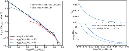
Left-hand panel: Comparison between the surviving unevolved subhalo mass function for two different parent halo masses at redshift z = 0. The coloured dashed lines are the results from decode, the solid lines are the results extracted from the Millennium simulation (as described in Section 2) and the solid black line the analytical form taken from Jiang & van den Bosch (2016). Right upper panel: fudge factor as function of the mass ratio according to equation (9). Right lower panel: merging time-scale from McCavana et al. (2012) (solid line) compared with that computed by applying the fudge factor correction (dashed–dotted line).
In order to be used as a flexible tool to model, e.g. galaxy merger rates, it is essential for decode to not only generate the correct abundances of subhaloes of different orders, but also to reproduce the correct probability distributions of their infall redshifts zinf. The left-hand panel of Fig. 3 shows the predicted zinf PDFs predicted by decode (histograms) for different subhalo masses and order, as labelled. As described in Section 3.3, these PDFs have been calculated by generating full merger trees for each parent halo and subhalo. Such a procedure is of course not practical and time-consuming. For this reason, we fit analytical functions to the PDFs of all second- and third-order subhaloes of different masses of interest here, and we report the best-fitting parameters for equation (3) in Table 1. We recall that the PDFs for first-order subhaloes are instead directly computed by the change of the SHMF along the parent halo mean mass accretion track (Section 3.4). The right-hand panel of Fig. 3 compares the number densities of the infall redshifts of first- and second-order subhaloes accreting on to a parent haloes of mass between |$10^{14}$| and |$10^{14.1} \, \mathrm{M}_\odot$| as predicted by decode (dashed lines) and the Millennium simulation (solid lines). The agreement is good, further validating the accuracy of our modelling.
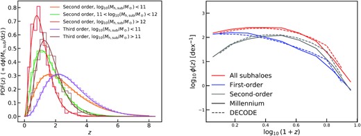
Left-hand panel: analytical (normalized) probability distributions of the infall redshifts adopted in this work to generate the mock catalogues. The results are organized for different subhalo orders and mass ranges. The histograms show the results from the merger tree and the curves show the best fits. Right-hand panel: comparison between number densities of the infall redshifts from our model decode (dashed lines) and from Millennium simulation (solid lines) for parent haloes of mass selected between |$10^{14}$| and |$10^{14.1} \, \mathrm{M}_\odot$|. Results are shown for subhaloes of all orders (red lines), first order (blue lines), and second order (grey lines). Similar results are found for other parent halo masses.
Best-fitting parameters of the infall redshift distribution parametrization from equation (3), for different subhalo orders and mass intervals.
| Subhalo order | Mass range | A | α | β | γ | δ |
|---|---|---|---|---|---|---|
| Second | 10 < log10(Mh,sub/M⊙) < 11 | |$10.06_{-3.86}^{+3.51}$| | |$1.07_{-0.14}^{+0.16}$| | |$13.78_{-5.78}^{+3.51}$| | |$1.86_{-7.80}^{+9.25}$| | |$1.77_{-0.37}^{+0.44}$| |
| Second | 11 < log10(Mh,sub/M⊙) < 12 | |$24.93_{-10.31}^{+6.24}$| | |$1.77_{-0.18}^{+0.22}$| | |$8.87_{-3.64}^{+3.39}$| | |$0.42_{-6.71}^{+6.22}$| | |$1.94_{-0.35}^{+0.43}$| |
| Second | log10(Mh,sub/M⊙) > 12 | |$24.81_{-9.19}^{+5.64}$| | |$2.67_{-0.21}^{+0.26}$| | |$2.31_{-0.87}^{+0.88}$| | |$-2.60_{-4.08}^{+2.52}$| | |$1.86_{-0.34}^{+0.45}$| |
| Third | 10 < log10(Mh,sub/M⊙) < 11 | |$8.37_{-3.36}^{+2.76}$| | |$1.50_{-0.18}^{+0.21}$| | |$13.50_{-5.79}^{+3.74}$| | |$3.00_{-8.75}^{+10.33}$| | |$3.29_{-0.51}^{+0.53}$| |
| Third | log10(Mh,sub/M⊙) > 11 | |$23.71_{-12.63}^{+7.73}$| | |$2.54_{-0.31}^{+0.31}$| | |$3.41_{-1.70}^{+1.57}$| | |$-3.56_{-4.65}^{+4.59}$| | |$3.12_{-0.49}^{+0.70}$| |
4 RESULTS
As introduced in the previous Sections, decode is a flexible statistical SEM that can predict, for a given input SMHM relation, the implied star formation and merger histories of central galaxies. It is in concept similar to its predecessor, steel, but it has relevant new features, including the separation in subhalo accretion order and a more refined treatment of infall time-scales.
In this work we will mostly focus on the ability of decode to rapidly predict the mean merger histories of central galaxies of different stellar mass for different input SMHM relations. In a separate work, we will extend decode to predict star formation histories and the amount of intracluster light generated from the stellar stripping of infalling satellites.
G20 identified a major role played by the SMHM relation in shaping the merger history of a central galaxy, especially in the case of more massive galaxies. In brief, if the high-mass end of the SMHM is flatter, it will imply that a halo increasing with mass via mergers will correspond to progressively lower growth in the stellar mass of its central galaxy. In the extreme condition of a perfectly flat SMHM relation, any increase in halo mass would not be followed by any increase in stellar mass, i.e. the (especially major) merger rate of those type of central galaxies will be drastically reduced.
In this Section, we further expand on G20 taking into account the different SMHM relations as derived from abundance matching using the latest data on the SMF at low and high redshifts (Section 4.1). We will then discuss the implied merger rates (Section 4.2), number densities of ‘unmerged galaxies’, i.e. satellites, in the local Universe for different SMHM relations (Section 4.3), the implied fraction of ellipticals originating from major mergers (Section 4.4), and the distribution of B/T stellar mass ratios of galaxies in the local Universe induced by major mergers and some models of disc instabilities (Section 4.5). We will also present the prediction of the growth histories of BCGs in Section 4.6. We will show that, as expected, the aforementioned quantities are highly dependent on the input SMHM relation in a hierarchical DM-dominated framework of galaxy evolution.
4.1 Stellar mass–halo mass models
As anticipated above, and further discussed in detail by many groups (e.g. Wang & Jing 2010; Guo et al. 2011; Moster et al. 2010, 2013), the SMHM relation is strongly dependent on the shape and evolution of the measured SMF. Unfortunately, the latter is far from known with sufficient accuracy, not even in the local Universe. Bernardi et al. (2013, 2016, 2017), for example, showed that the SMFs in SDSS and CMASS at z = 0.1 and z = 0.5, respectively, are highly dependent on the light profile chosen to fit the photometry. When the same methodology is consistently applied to infer stellar masses, no apparent evolution is detected in the high-mass end of the SMF up to at least z = 0.5–0.8 (see also Shankar et al. 2014), whilst significant evolution at all masses is inferred when comparing Bernardi et al. (2017) and, e.g. Davidzon et al. (2017), who derived stellar masses from SED fitting. Additional systematic differences in SMFs have been claimed by, e.g. Leja et al. (2020), who support larger stellar masses at fixed SFR. The substantial systematic uncertainties in measured SMFs naturally propagate into the shape, scatter, and evolution of the SMHM relation. In what follows, we present four models for the SMHM relation derived from direct abundance matching, as detailed in Section 3.5, with different observed SMFs. Our aim is to estimate to what extent observationally informed systematic differences in the input SMHM relation impact the implied galaxy merger rates and bulge fractions, a task that is particularly suited to address with decode. The four SMHM models considered in this work can be summarized as follows:
Model 1:
Bernardi et al. (2017) SMF, assumed to be constant up to z ≈ 1.5. This is of course an extreme assumption but worth exploring as it is still unclear whether apparent evolution in the SMF at z > 0 may be, at least in part, driven by non-ideal/inconsistent estimates of galaxy stellar masses, as mentioned above. Indeed, Kawinwanichakij et al. (2020) recently suggested that there is no measurable evolution in the SMF up to at least z = 1.5.
Tinker et al. (2008) HMF.
0.15 dex constant scatter in stellar mass at fixed halo mass.
Model 2:
Tomczak et al. (2014) SMF at z > 0 and Bernardi et al. (2017) at z = 0. This model is also somewhat extreme because, as detailed above, the z > 0 SMF estimates may be affected by systematic measurement errors and/or incomplete. Nevertheless Models 2 and 1 should bracket the range of possible evolutionary patterns of the SMF, at least based on the present data and on the assumption of a constant IMF.
Tinker et al. (2008) HMF.
0.15 dex constant scatter in stellar mass at fixed halo mass.
Model 3:
- equivalent to Model 1 but assuming a linearly increasing scatter with redshift up to z = 2 as follows:(10)$$\begin{eqnarray} \left\lbrace \begin{array}{l}\sigma _{\log M_*} = 0.15 + 0.1 z \,\,\,\,\,\, {\rm for} \,\, z\lt 2\\ \sigma _{\log M_*} = 0.25 \,\,\,\,\,\,\,\,\,\,\,\,\,\,\,\,\,\,\,\,\,\,\,\,\,\, {\rm for} \,\, z \ge 2 \end{array} \right. \end{eqnarray}$$
Model 4:
equivalent to Model 2 but with the same z-dependent scatter as Model 3.
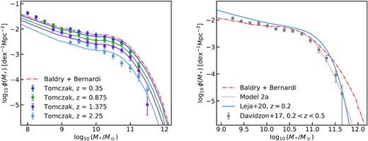
Stellar mass functions used for the abundance matching of the SMHM for the different models described in Section 4.1. In both panels, the red dashed–dotted line represents the combination of the SMF from Baldry et al. (2012) and Bernardi et al. (2017) at z = 0.1. In the left-hand panel, the dots with error bars represent the observational data from Tomczak et al. (2014) and the coloured solid lines the redshift-dependent normalization correction (equation 12) applied to the Baldry + Bernardi SMF to be consistent with the Tomczak + 14 data at z > 0. In the right-hand panel, the dots with error bars show the data from Davidzon et al. (2017), while the blue solid line and red dotted line show the SMF from Leja et al. (2020) and the correction (as described in Section 4.1) to the Baldry + Bernardi SMF for being consistent with the Davidzon + 17 data, respectively.
Given the SMFs at any given epoch z < 4 and for each Model, it is now necessary to specify the host halo mass functions to then apply the abundance matching routine given in equation 8. We choose the Tinker et al. (2008) HMF, which provides the abundances of host parent haloes (we note that switching to other forms of the HMF would yield very similar results throughout). As the SMFs at z > 0 contain both central and satellite galaxies (though the latter become progressively negligible in number densities at earlier epochs), we need to correct the Tinker et al. (2008) HMF by the abundances of surviving satellites at any epoch of interest, as specified in Section 3.5.
The SMHM relations, derived from our abundance matching algorithm for each Model, are shown in Fig. 5 in the redshift range 0 < z < 3. Models 1 and 3 are characterized by a high-mass slope dlog10(M*/M⊙)/dlog10(Mh/M⊙) (between |$M_{\rm h} = 10^{13}$| and |$M_{\rm h} = 10^{14} \, \mathrm{M}_\odot$|) of 0.550, and a low-mass one (between |$M_{\rm h} = 10^{11}$| and |$M_{\rm h} = 10^{11.5} \, \mathrm{M}_\odot$|) of 1.30, both with a normalization of 10.509 at |$M_{\rm h} = 10^{12} \, \mathrm{M}_\odot$|, at z = 1. Models 2 and 4 instead have a high-mass slope of 0.588 and 0.508, a low mass slope of 1.15, and a normalization of 10.138 and 10.163, respectively. As shown in Fig. 5, our Model 2 at z = 0 is very close to both Moster et al. (2018) and Behroozi et al. (2019), at least at high stellar masses. The main difference between Model 2a and the others is the significantly flatter slope of 0.414 at the high-mass end. We will show below that such apparently small differences in the shape of the SMHM relations, especially the differences in the slopes at the high-mass end of the SMHM relations, are sufficiently large to generate significant systematic differences in, e.g. the major merger rates and implied elliptical fractions of up to a factor of 2–4 in some stellar mass bins. We notice that by keeping the SMF constant in time (Models 1 and 3) induces a weak evolution at low masses and a more pronounced one at larger masses. On the other hand, the models characterized by an evolving SMF (Models 2 and 4), generate an SMHM relation with evident redshift evolution at low stellar masses and a weak one at higher stellar masses (see also Shankar et al. 2006; Moster et al. 2018, G20).
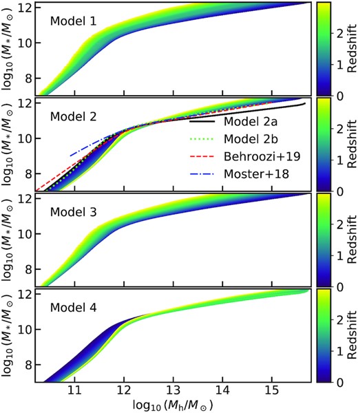
Stellar mass–halo mass relations computed via abundance matching. The four panels show the relations for the four models described in Section 4.1, respectively, for the range of redshift denoted by the colour code. In the second panel, we show also Models 2a and 2b, along with two SMHM relations from other works in the literature (Moster et al. 2018; Behroozi et al. 2019) for comparison (black solid, green dotted, red dashed, and blue dashed–dotted lines, respectively).
4.2 Merger rates
The input SMHM relation has a direct impact on the merger rate of each galaxy that decode produces (e.g. Stewart et al. 2009b; Hopkins et al. 2010b; Grylls et al. 2020b; O’Leary et al. 2021), which in turn influences the implied satellite abundances, fraction of ellipticals, and B/T ratios. In this Section, we focus on galaxy merger rates and other predictions will be discussed in the following Sections.
First of all, we checked that our halo–halo merger rates are consistent with the halo–halo merger rates derived by Fakhouri et al. (2010) from the Millennium simulation at z ≳ 0.35. We note that our fits drop slightly faster than those of Fakhouri et al. (2010) at z < 0.35, as also previously noted by G20, which we checked is mostly induced by our adopted halo mass mean accretion histories from van den Bosch et al. (2014) which are somewhat steeper than those presented in Fakhouri et al. (2010) at these redshifts. Fig. 6 shows the cumulative number of total and major mergers from decode (upper and lower panels, respectively) below z < 4 predicted from decode, expected in a hierarchical ΛCDM Universe, as a function of parent halo mass. We found that the number of mergers, with both first- and second-order subhaloes, is roughly constant with parent halo mass (see also Shankar et al. 2014). However, such an invariance in halo mass is broken when mapping DM halo mergers to galaxy mergers via the double power-law shaped SMHM relation. We show this result in Fig. 7, where we plot the average number of major mergers, along with its 1σ uncertainty, as a function of the (final) galaxy stellar mass. The red lines represent the contribution of mergers from first-order satellites and the blue lines the contribution of mergers from second order. The plot clearly shows that, for all the four SMHM models, the contribution from the second-order satellites is in good approximation relatively negligible, at least for massive central galaxies. On the other hand, the number of mergers from the first-order satellites increases significantly when the central galaxy mass increases.
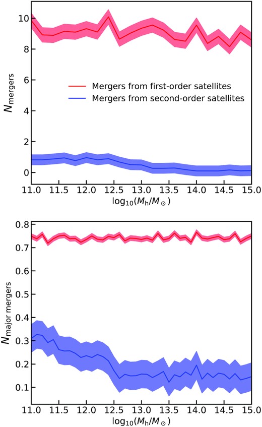
Upper panel: number of dark matter mergers from the contribution of first- and second-order subhaloes as function of the final parent halo mass at redshift z = 0. The solid lines represent the mean value, while the shaded areas show the 1σ uncertainty. Lower panel: same as upper panel, but for major mergers, for which we assume a mass ratio Mh,sub/Mh,par > 0.25.
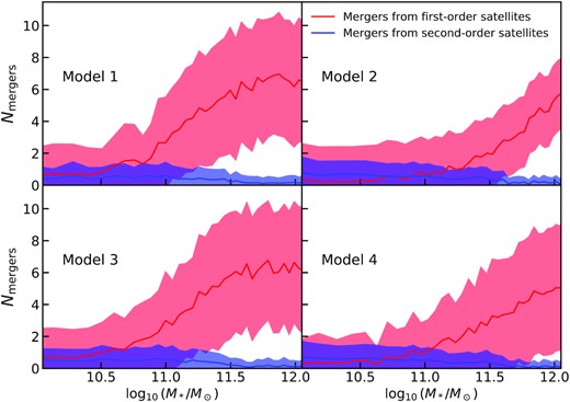
Number of galaxy major mergers from first- and second-order satellites, with mass ratio M*,sat/M*,cen > 0.25, as a function of the central galaxy mass. The solid lines represent the mean value, while the shaded areas show the 1σ uncertainty. Results are shown for the four different models described in Section 4.1, as labelled.
The sharp increase of major mergers with galaxy stellar mass and the fact that major mergers for massive galaxies outnumbers the major mergers of the parent haloes can be both explained from the shape of the SMHM relation. Indeed, while the total number of mergers is the same for the DM halo and the host galaxy (and it is independent of the halo or stellar mass), the classification as major or minor merger depends on the mass ratio between halo or stellar mass (Mh,1/Mh,2 > 0.25 is the major merger threshold for halo mergers and M⋆,1/M⋆,2 > 0.25 for galaxy mergers). Since the SMHM relation sets |$M_\mathrm{h}\propto M_\star ^\alpha$|, the halo mass ratio is related to the stellar mass ratio as Mh,1/Mh,2 = (M⋆,1/M⋆,2)α. If the SMHM relation was linear (α = 1) the halo mass ratio would be equal to the stellar mass ratio and, consequently, a halo major merger would correspond to a galaxy major merger. On the other hand, a steep power-law relation with α > 1 would decrease the stellar mass ratio with respect to the halo mass ratio, while a flat power law with α < 1 would increase it. As a consequence, the number of galaxy major mergers is reduced for a steep power law, while it is enhanced for a flat one. In other words it is less (more) likely to find similar mass galaxies for similar mass haloes for a steep (flat) SMHM. Since the SMHM relation in all the four considered models is a broken power law with a steep faint end and a flat bright end, the number of galaxy major mergers tends to naturally increase towards higher stellar masses. However, the level of increase is different for the four models since even small variations in the SMHM relation produce strong effects in the merger rates. For example, Model 2 with a high-mass slope of 0.558 predicts less than half of the mergers at |$M_* \sim 1-3 \times 10^{11} \, \mathrm{M}_\odot$| compared to Model 1 and Model 3 with a high-mass slope of 0.550. On the other hand, Model 4, despite having the lowest high-mass end slope at z = 0, produces slightly more mergers than Model 2 but less than Models 1 and 3, a trend that can be explained by the lower slope in the SMHM relation at higher redshifts in Model 4 than in Model 2, being e.g. 0.498 and 0.551 the average slope up to z = 1.5, respectively. For more massive galaxies, Models 1 and 3 predict on average a higher number of major mergers compared to Models 2 and 4. This effect is also directly reflected in the fraction of ellipticals and B/T ratios, as we will see in the following Sections. We also note that, although the normalization of the SMHM does not directly impact the number of major mergers, it has an important role in determining the total merger history, which in turns will impact the star formation history, as we will discuss in future work. Furthermore, the amount of scatter in the SMHM relation instead seems to play a relatively less significant role in controlling the fraction of major mergers when assuming a constant SMF.
Furthermore, we show in the upper panel of Fig. 8 the major merger pair fraction as predicted by decode for Models 1, 2, and 2a. We compare our results with the data from UKIDSS UDS, VIDEO/CFHT-LS, UltraVISTA/COSMOS, and GAMA surveys, presented in Mundy et al. (2017). The pair fraction in decode is calculated as the number of infalling satellites with stellar mass ratio above 1/4 living within 5 and 30 kpc from the centre of the central galaxy. We assume that the distance of the satellite galaxies scales proportionally to its dynamical friction time-scale (Guo et al. 2011). We make use of the projected 2D distances computed following the recipe in Mundy et al. (2017) and Simons et al. (2019), assigning stochastically a polar angle in spherical coordinates and projecting the 3D distances on to the z-axis. Analogously to what inferred for the number of major mergers, Model 1 tends to produce more pair fractions with μ > 1/4 than Model 2. The available data on pairs is still sparse, and still subject to systematics in the determination of the stellar masses, but overall Model 2 tends to be more aligned with the data, at least at z ≥ 0.5. On the other hand, Models 1 and 2a, characterized by a flatter slope in the SMHM relation at the high-mass end, predict a higher pair fraction with respect to the data and to Model 2. This prediction is in line with the fact that a flatter SMHM relation produces a higher number of major mergers, as discussed above.
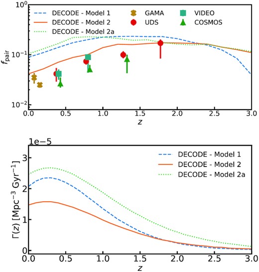
Upper panel: major merger pair fraction, with mass ratio μ ≳ 0.25, for galaxies at |$M_* \gtrsim 10^{11} \, \mathrm{M}_\odot$| as predicted by decode for Models 1, 2, and 2a (blue dashed, orange solid, and green dotted lines, respectively). The points with error bars show the observational data of UDS, VIDEO, COSMOS, and GAMA surveys, as presented in Mundy et al. (2017). Lower panel: major merger rates as a function of redshift, as predicted by decode’s Models 1, 2, and 2a.
Finally, in the lower panel of Fig. 8 we show a prediction of the major merger rates from decode’s Models 1, 2, and 2a. As we can see, the flatter the SMHM relation (Models 1 and 2a) the higher the rate of implied major mergers, in line with what shown in the upper panel. On the other hand, Model 2, characterized by a steeper SMHM high-mass end, predicts a much lower major merger rate, at least at lower redshifts. We do not show the comparison with observational data or any other model because the merging time-scales that we use (McCavana et al. 2012) are different to those adopted in other theoretical and observational works.
In the next Sections we will show and discuss how the different shapes and evolution of the input SMHM relation play a crucial role in determining the satellite abundances, fraction of ellipticals, and B/T ratios.
4.3 Predicting the abundances of satellite galaxies
Having defined the mapping between galaxy stellar mass and host DM halo mass, we can start to predict galaxy observables that can be used to validate decode and the input SMHM relation. As a very first test, we compute the number density of surviving satellite galaxies in the local Universe and compare it with SDSS data. Satellites can be effectively considered as the other side of the same coin with respect to mergers. In fact, surviving satellites in a hierarchical DM-dominated Universe, can be interpreted as ‘failed mergers’, i.e. all those infalling satellite galaxies that have not yet had the time to merge with their central galaxies at the time of observation. Therefore satellites, just like mergers, represent a pivotal test of hierarchical models and of the input SMHM relation. Although the total SMF is an input in decode, the satellite SMF is an actual prediction of the model, as it depends both on the satellite evolution after infall and on the rate of galaxy mergers, which in turn depend on the high-z SMHM relation and on the dynamical friction time-scales.
Fig. 9 shows the results of the SMF for all galaxies (centrals + satellites) and only satellites (red and blue lines, respectively). The different types of line distinguish the four SMHM models, and the blue and red dots with error bars are, respectively, the satellite9 and total galaxy SMF as measured in SDSS using, for consistency with our Models, the data from Bernardi et al. (2017). As one can see from the red lines, the total SMF is well reproduced by decode, as expected by construction via the abundance matching relation given in equation (8). For all SMHM models reported in Fig. 5, we assume a ‘frozen’ scenario in which satellite galaxies are assumed to retain the same stellar mass after infall with no further growth via star formation or loss via, e.g. stellar stripping. G19 showed that the frozen model was able to reproduce the bulk of the observed satellite population in their SEM steel. We do find a similar result with decode in Fig. 9, despite using a significantly more accurate distributions of satellites of first and second order and dynamical friction time-scales. We will explore in separate work the impact of star formation and stellar stripping on the satellite population and star formation histories. We anticipate here that including standard recipes for stellar stripping as given by, e.g. Cattaneo et al. (2011), and for star formation after infall following the analytic recipes by G20 (and references therein), we obtain very similar results to those shown in Fig. 9. Fig. 9 shows that only Model 2, the one characterized by an evolving SMF and constant scatter, better lines up with the observational data of satellites, especially at stellar masses |$M_* \gtrsim 3 \times 10^{10} \, \mathrm{M}_\odot$|. We will see below that Model 2 also performs better against other observational constraints.
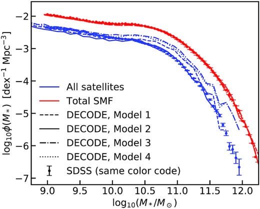
Total and satellite galaxies stellar mass function predicted by decode compared to the data from SDSS. The solid, dashed, dashed–dotted, and dotted lines show the prediction for Models 1, 2, 3, and 4, described in Section 4.1, respectively. The dots and error bars represent the data from SDSS.
4.4 Morphology of central galaxies
In this section, we apply decode to study another key aspect of galaxy evolution: the role of mergers in shaping galaxies, and in particular in generating elliptical type galaxies. Many works have in fact suggested a close link between the number of major mergers and the number of ellipticals (e.g. Bournaud et al. 2007; Hopkins et al. 2009a, 2010a; Shankar et al. 2013; Fontanot et al. 2015). Major mergers (for which we assume f = M*,sat/M*,cen ≳ 0.25) may be capable of destroying pre-existing galactic discs and form stellar spheroids, as suggested by hydrodynamical simulations and analytical models (see e.g. Baugh 2006; Malbon et al. 2007; Bower et al. 2010; Tacchella et al. 2019; Lagos et al. 2022). However, as discussed by G20 and above, as the number of major mergers is strongly dependent on the shape of the input SMHM relation, we expect the fraction of ellipticals to be similarly impacted by the choice of SMHM relation. We will investigate this possibility in this Section.
For each SMHM model, we follow the merger history of galaxies in the mock from redshift z = 4, and we label each galaxy that has undergone a major merger as an ‘elliptical’, and then compute the fraction of ellipticals at different redshifts. We show the results in Fig. 10. Panels A, B, and C show the fraction of ellipticals predicted by decode using the four Models of SMHM described in Section 4.1 for redshifts z = 0.1, 1, and 2, respectively, along with the predictions from the TNG simulation and from the semi-analytical model galics, as well as with the SDSS data (see Section 2.4), only shown in the panels at z = 0.1. We note that, as discussed in Section 2, galics and TNG define elliptical galaxies in a somewhat different way than a simple cut in μ, but we still include their predictions in Fig. 10 for completeness.
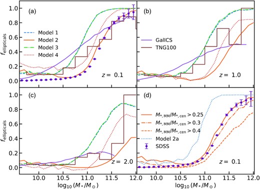
Fraction of elliptical galaxies as a function of the galaxy stellar mass as predicted by decode. Panels A, B, and C show the predictions for the four models described in Section 4.1 at redshifts z = 0.1, 1, and 2, respectively. Panel D shows the predictions for Model 2 at redshift z = 0.1, along with the impact of assuming different mass ratio for the major mergers (denoted as MM in the legend), as well as the prediction for Model 2a. The data from the SDSS survey, galics semi-analytical model and the TNG100 hydrodynamical simulation are included, as labelled, for comparison.
It is immediately clear from Fig. 10 that Model 2 is the only one among our four chosen SEMs that can faithfully reproduce the SDSS data at z = 0.1, on the assumption that ellipticals are strictly formed from major mergers above a mass ratio of μ > 0.25, the standard limit adopted in state-of-the-art SAMs (e.g. Guo et al. 2011; Fontanot et al. 2015; Lacey et al. 2016). Model 4, which only differs from Model 2 on the assumed scatter around the SMHM relation, is moderately close, but still higher than the data for the same cut in merger ratio μ > 0.25, further proving that even a modest variation in the scatter of the SMHM relation can significantly impact galactic outputs. In particular, an increase of the scatter at fixed slope at high stellar masses tends to increase the number of major mergers. On the other hand, Models 1 and 3 produce a significantly higher fraction of ellipticals. The main reason why models including evolution in the SMF predict less elliptical galaxies than models with constant SMF is a direct consequence of the number of mergers that they predict, as discussed in Section 4.2. Fig. 10 also shows that the TNG100 simulation provides a decent match to the SDSS at z = 0.1, especially at galaxy masses |$M_* \gt 2 \times 10^{11} \, \mathrm{M}_\odot$|, although we should caution that some internal self-inconsistencies naturally arise when comparing with the TNG100 outputs with these data as the TNG100 simulation does not exactly reproduce the same SMF of Bernardi et al. (2017) (see e.g. Pillepich et al. 2018b), on which the elliptical fractions are based, and thus has an SMHM relation that slightly differs from the one in Model 2. The SAM galics10 also well matches the SDSS elliptical fractions at high stellar masses, but it overproduces them at lower stellar masses. Lastly, we show in panel D of Fig. 10 the fraction of ellipticals predicted by Model 2a. This model, characterized by a flatter high-mass end slope, produces a much larger number of mergers, as expected from the discussion in Section 4.2, and thus it increases the implied fraction of ellipticals at all stellar masses.
In conclusion, the question whether major mergers are the triggers for the formation of local ellipticals, is strongly dependent on the SMHM relation in input or generated by the model in use, and, at fixed SMHM relation, on the exact threshold chosen for being classified as a major merger, as shown in panel D.
Finally, we show for completeness the fraction of lenticular-type galaxies as a function of stellar mass in Fig. 11 predicted from decode for Model 2, compared with the observational data from SDSS. Several works have suggested that lenticular galaxies might be created by mergers as well (e.g. Christlein & Zabludoff 2004; Laurikainen, Salo & Buta 2005; Blanton & Moustakas 2009). Here, we label the lenticulars as the galaxies that have had at least one merger with mass ratio 0.05 < μ < 0.25, whilst above μ = 0.25 they would end up as ellipticals. This simple merger recipe is capable of reproducing the data for stellar masses |$M_* \gtrsim 10^{11} \, \, \mathrm{M}_\odot$|, but it fails at lower stellar masses, suggesting that additional processes may be at work in forming less massive lenticulars, such as disc instabilities and/or disc regrowth.
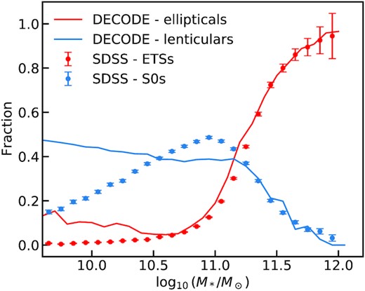
Fraction of lenticular and elliptical galaxies as predicted by decode for Model 2 compared with the data from theSDSS Survey, as labelled.
4.5 Bulge-to-total ratios
In the previous sections, we showed that the shape of the SMHM relation drives the number and thus the rate of mergers galaxies undergo through cosmic time (at fixed dynamical friction time-scale). Only specific SMHM relations, such as the one defined in Model 2, which is characterized by a larger number density of massive galaxies and a significant evolution in normalization at z > 0.5 − 1, are able to simultaneously reproduce the number of local satellites and the number of local ellipticals, on the assumptions that the latter are formed out of mergers between galaxies with a mass ratio M*,1/M*,2 > 0.25. We now move a step forward in our modelling and test how well our Models 1 and 2 reproduce the B/T ratios of local galaxies, as measured in MaNGA (see Section 2).
To perform a meaningful and instructive comparison between models and data, we make use of two simple but theoretically well-motivated toy models for the formation of bulges in hierarchical models:
In Model BT1, we assume that when a major merger occurs, with M*,1/M*,2 > 0.25, the descendant galaxy is strictly an elliptical with B/T = 1. This is a common assumption made in semi-analytical models of galaxy evolution (e.g. Cole et al. 2000; Hatton et al. 2003; Bower et al. 2006; De Lucia & Blaizot 2007; Guo et al. 2011; Croton et al. 2016; Lacey et al. 2016; Cattaneo et al. 2017). We then assume that in minor mergers the mass of the satellite can be accreted either on to the bulge or on to the disc component.
In Model BT2, we instead assume that the remnant galaxy has a surviving disc with B/T = 0.5. In other words, we assume that the disc is not entirely disrupted in a major merger, irrespective of the gas fraction in the progenitor galaxies, but in fact a significant fraction of it survives and/or is rapidly reaccreted (e.g. Hopkins et al. 2009b; Puech et al. 2012). We then explore the impact on the final B/T of assuming the satellite mass in minor mergers to be added systematically to the disc or to the bulge component. We note that, in what follows, we consider the B/T at fixed galactic stellar mass averaged over all central galaxies that enter that bin in stellar mass.
The top panels of Fig. 12 report our results for the merger Models BT1 and BT2, for the SMHM relation in Model 1 (left-hand panel) and Model 2 (right-hand panel), shown with cyan- and orange-shaded areas, respectively, where the upper and lower bounds mark the limiting cases where all the stellar mass of the minor merger is transferred to the bulge and to the disc, respectively, and the dashed lines represent the mean of the two cases. We compare our predictions with data on the mean B/T as a function of galaxy stellar mass from MaNGA (black dots with error bars), as detailed in Section 2.4. The fact that the shaded areas in SMHM Model 2 are slightly broader at high stellar masses than those in Model 1 is an artefact of the number of mergers predicted by these Models, as shown in Figs 6 and 7. In particular, at fixed number of DM mergers, Model 2 predicts less major mergers, i.e. more minor mergers than Model 1. This leads to a higher bulge/disc mass in the cases where all the mass from minor mergers goes to the bulge/disc, leading, therefore, to a larger bound.
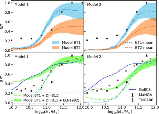
Mean bulge-to-total ratios for the two different toy models described in Section 4.5 and SMHM relationships of Models 1 and 2. The blue and orange shaded areas in the upper panels show the results for Models BT1 and BT2 (for Models 1 and 2, respectively), while the green areas in the lower panels show the results for Model BT1 but by including disc instabilities of Efstathiou et al. (1982) (equation 15). The dashed tick green lines show the B/T ratios for Model BT1 by including only Bournaud et al. (2011) disc instabilities. The shaded areas are constrained by the two limit cases, where all the mass from minor mergers goes into the bulge and disc, respectively, and the thin dashed lines show the mean. The black error bars represent the 1σ bound from the MaNGA survey. Finally, the blue solid line shows the prediction from galics semi-analytical model and the brown triangles with error bars the results from the TNG simulation. The uncertainties for the MaNGA survey and the TNG simulation are estimated using the standard deviation on the median.
The MaNGA data clearly indicate that all local galaxies have a B/T ratio that is confined within 0.2–1, with a mean value slightly rising with increasing stellar mass, from ∼0.2 reaching an average value of B/T ∼ 1 only in the most massive galaxies with |$M_* \gtrsim 10^{11} \, \mathrm{M}_\odot$|. Models that, like our BT1, assume a strict B/T = 1 during major mergers, can better reproduce the data at high stellar masses, especially when assuming that all the minor mergers contribute to the bulge component. On the other hand, models that, like BT2, assume that a significant fraction of the disc survives and/or is rapidly reaccreted after the merger, fall short in matching the data at high stellar masses, suggesting that these kinds of model are not extremely suitable to describe the average B/T ratios, at least at high stellar masses.
Irrespectively of what we assume for the B/T in major (or even minor) mergers, both our BT1 and BT2 Models drastically fail in reproducing the observed B/T in galaxies with |$M_* \lesssim 2 \times 10^{11} \, \mathrm{M}_\odot$| (top panels of Fig. 12). An additional component/process should be included in decode to reproduce the data. Here, again we can witness the usefulness of a semi-empirical approach that, as discussed in the Section 1, can include additional layers of complexities wherever necessary, as guided by the data, in a transparent and efficient way. The bottom panels of Fig. 12 show the prediction of Model BT1 by including disc instabilities as discussed above. We do not show Model BT2 as it fails to model the B/T ratios even with the addition of disc instabilities. The main effect of including disc instabilities in our Model BT1 is that it tends to increase the bulge masses at lower, but not at higher, galaxy stellar masses, where the condition in equation (15) is more easily met mainly because lower mass galaxies retain their disc morphologies for a longer time. In particular, we find that, irrespective of the exact input SMHM relation, to broadly match the data we need to assume that a fraction of the disc mass is transferred to the bulge at each disc instability event, in line with some previous cosmological models (e.g. Bower et al. 2006). In the bottom panels of Fig. 12, we show both the cases where clumpy accretion (following Bournaud et al. 2011) and ‘classical’ disc instabilities (Efstathiou et al. 1982) are implemented. We find that Model BT1,12 the one without disc regrowth, with SMHM Model 2 broadly matches the SDSS local average B/T ratios when some level of disc instabilities is included in the model, while it fails to match the data at low masses with SMHM Model 1. In particular, disc instabilities implemented following Bournaud et al. (2011) appear not to be sufficient to provide enough boost to the average B/T at the low-mass end to match the data, even if the baryonic inflow rate in equation (14) is doubled. On the other hand, disc instabilities as in Efstathiou et al. (1982) allow to broadly reproduce the observational data of SDSS, when the factor ϵ in equation (15) is roughly 0.5. Intriguingly, one could argue that strong disc instabilities, and not necessarily major mergers, are responsible for forming most stellar bulges, even at the highest stellar masses. In fact, the strength of a disc instability in forming a bulge closely depends on the D/T ratio, the more disc mass there is, the more potential there is for the bulge to grow in mass after a disc instability. We however checked that even on the assumption of ineffective major mergers preserving a B/T ∼ 0.2, the disc instabilities would still fall short in boosting the B/T up to unity at high stellar masses.
In the bottom panels of Fig. 12, for completeness, we compare our predictions with the outputs from the TNG100 simulation and the galics SAM (brown triangles with error bars and blue solid line, respectively). Interestingly, both TNG100 and galics predict large mean B/T ≳ 0.9 at high stellar masses in reasonable agreement with our predictions and the data. In addition, they also include bulge formation via disc instabilities (see e.g. Tacchella et al. 2019; Cattaneo et al. 2020), predicting indeed B/T > 0.2 at low masses in line with the data, though the mean B/T predicted by galics tends to be larger than the one measured in MaNGA towards lower stellar masses (we provide in Appendix D a detailed comparison between the B/T ratio found in MaNGA and those from other samples/studies). Our Model 1 is roughly consistent with the predictions of galics at all masses but not with the observational data and the TNG simulation at low masses, while Model 2 behaves in nearly the opposite fashion, highlighting once again the dependence of galactic properties, this time the mean B/T ratios, on the input SMHM relation.
Finally, in Fig. 13 we show the mean mass growth of bulges and discs for four galaxy masses at z = 0 for Model BT1 with and without disc instabilities, as labelled. We note that, when disc instabilities are not included, at low stellar masses (e.g. |$M_*(z=0) \sim 10^{10.5} \, \mathrm{M}_\odot$|) the disc dominates the overall mass growth of the galaxies and the bulge component is almost negligible, unless disc instabilities are included (long-dashed orange lines). Moving towards higher stellar masses, the bulge begins to be gradually more dominant, as a direct consequence of the increasing number of mergers, and adding disc instabilities does alter this trend noticeably.
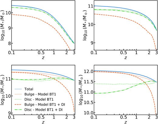
Average growth of total, bulge and disc stellar mass for four different galaxy mass bins at z = 0. The solid blue lines show the total stellar mass growth. The thin dashed and dashed–dotted lines show the mass growth of the bulges and discs, respectively, for Model BT1, while the thick lines show the mass growths for Model BT1 including disc instabilities.
4.6 Brightest cluster galaxies history
As a final application of decode, we study the stellar mass growth history of BCGs, which are massive elliptical galaxies that constitutes an additional source of information for understanding the evolution of galaxies and large-scale structure. Several studies have addressed already this issue, both from observations (e.g. Whiley et al. 2008; Collins et al. 2009; Stott et al. 2010; Lidman et al. 2012; Bellstedt et al. 2016; Lin et al. 2017; Zhang et al. 2017) and numerical works, such as SAMs (e.g. De Lucia & Blaizot 2007; Contini et al. 2014), SEMs (Shankar et al. 2015), and hydrodynamic simulations (e.g. Pillepich et al. 2018b; Ragone-Figueroa et al. 2018). Here, we show the predictions of decode for the stellar mass assembly of BCGs and how these compare to the results from other works.
The results are shown in Fig. 14. The red dashed and solid lines show the total stellar mass fractional growth of BCGs, selected in haloes with present-day mass |$M_{\rm h} (z=0) \gt 8 \times 10^{14} \, \mathrm{M}_\odot$|, predicted by decode with Models 1 and 2, along with their 1σ uncertainties (shaded areas). The data are compared with the COSMOS data (Cooke et al. 2019), results from the hydrodynamic simulations of Ragone-Figueroa et al. (2018) and SAM of Contini et al. (2014) (as labelled in the figure), selected in the same mass region. According to Model 1 BCGs have already formed most of their mass at redshifts z > 1.5, because of the assumed constant SMF up to that redshift which maps the DM halo mass accretion history into a higher average stellar mass growth. On the other hand, assuming Model 2 BCGs have only formed roughly |$50 {{\ \rm per\ cent}}$| of their mass by z = 1.5 and have grown the remaining mass at later epochs.
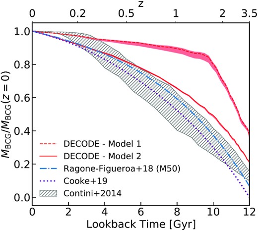
Fractional stellar mass growth of BCGs predicted by decode for Models 1 and 2 as a function of lookback time with their 1σ bounds (red lines and shaded areas). The blue dashed–dotted line corresponds to the fit M50 selected BCGs according to equation (2) in Ragone-Figueroa et al. (2018). The purple dotted line shows the observed median growth from COSMOS as presented in Cooke et al. (2019). The grey dashed area includes the evolutionary histories of the models in the Contini et al. (2014) semi-analytical model.
The BCG stellar masses in Ragone-Figueroa et al. (2018) are computed with the mass within the spherical radius of 50 kpc (M50). Our Model 2 is in relatively good agreement on the mass formation history of BCGs with M50 selected galaxies, predicting a factor of ∼1.5 in the mass increase between z = 1 and z = 0 against the factor 1.4 of Ragone-Figueroa et al. (2018).
Fig. 14 shows that models characterized by a SMHM relation with a significantly evolving underlying SMF as in Model 2, are once again better tuned to reproduce the current data, this time data on BCGs, in line with predictions from hydrodynamic simulations and SAMs. We note that in all our Models satellites are frozen. Increasing their masses via residual star formation after infall would possibly steepen the evolution for both Models, possibly slightly improving the match with the data for Model 1.
5 DISCUSSION
The discrete statistical and semi-empirical model, decode, presented in this work constitutes an invaluable complementary tool to the existing cosmological models for modelling galaxy evolution. These models, either analytical or numerical, are affected by significant volume/mass resolution limitations and/or a large amount of input assumptions and parameters. Also other existing works on SEMs, such as Behroozi et al. (2019) and Moster et al. (2018), based on abundance matching between galaxy–halo properties, still need large computational resources to run. Instead our model, based on statistical input distributions, allows to rapidly simulate a large volume box and investigate the mean properties of galaxies without relying on ab initio analytical models or simulations.
In the last decade several SEMs have been developed. We mention here some examples and discuss how decode differs from and complements them. Moster et al. (2018) showed an empirical relation between the mass growth of DM haloes and the galaxy star formation rate, from which they retrieve the mergers history and other properties. Moster et al. (2013) and Behroozi et al. (2019) proposed SEMs where they populate DM haloes via SMHM relations with galaxies in vast catalogues. These models connect galaxy to DM halo properties via several analytical relations, which could involve a non-negligible number of free parameters. Our present model, instead, although more restricted in scope as it only focuses on mean galaxy assembly histories, essentially relies on only one input parameter, the scatter in the SMHM relation. From this single parameter and abundance matching, decode can then generate robust predictions on mean galaxy growth histories, merger rates, satellite abundances, and star formation histories, thus providing a flexible and transparent tool to probe galaxy evolution in a full cosmological context. G19 recently developed an SEM where they apply abundance matching to statistical distributions of DM haloes and galaxies, which is limited by the non-discreteness since it is based on statistical weights over continuous probability densities. Our model instead applies the SMHM relation from abundance matching directly to the mock universe generated stochastically by making a realization of the distributions themselves.
The fact that decode starts from the SMF to compute the SMHM relation, makes decode a powerful tool to set more stringent constraints on the SMF. As discussed in Section 4.1, the galaxy SMF is far from being well known, especially at high redshifts, and many works suggested different (and sometimes contrasting) results, in terms of shape and/or evolution in time (e.g. Bernardi et al. 2013, 2016, 2017; Tomczak et al. 2014; Davidzon et al. 2017; Huang et al. 2018; Kawinwanichakij et al. 2020; Leja et al. 2020). Our current tests show a preference for SMFs characterized by a larger number of massive galaxies and a significant evolution in time. These SMFs generate SMHM relations that, in turn, produce a sufficient number of mergers to match the local fraction of ellipticals, satellite abundances, and BCG growth. Our study thus highlights the strong dependence of galaxy stellar mass assembly histories on the input SMHM relation. Stewart et al. (2009b) and Hopkins et al. (2010b) also found that galaxy merger rates depend on the input SMHM relation. Their results, along with ours, imply that, for a fixed DM merger tree, the major merger rates and other quantities strongly depend on the mapping between stellar mass and halo mass, which in turns depends on the systematics, shape and evolution of the SMF. Following their path, a fraction of |$~ 40{{\ \rm per\ cent}}$| of mass-loss during mergers can alter significantly the merger rates and, therefore, also the fraction of elliptical galaxies and B/T ratios, up to more than a factor of 2, which would allow also flatter SMHM relations to perform well.
In this work, we also found evidence for the need of disc instabilities to boost the formation of bulges at lower stellar masses. This result is in line with the general notion of fast and slow rotators (e.g. Bernardi et al. 2019; Domínguez Sánchez et al. 2020), which suggest that the former dominates at |$M_* \lesssim 10^{11.5} \, \mathrm{M}_\odot$| and the latter at |$M_* \gtrsim 10^{11.5} \, \mathrm{M}_\odot$|, or also with the distinction between pseudo- and classical bulges (see discussions in Gadotti 2009; Fisher & Drory 2010; Shankar et al. 2012, 2013, and references therein). Similar findings are retrieved in SAMs. Guo et al. (2011) found that at stellar masses |$M_* \gtrsim 10^{11} \, \mathrm{M}_\odot$| mostly all galaxies have a B/T > 0.7, and mostly B/T < 0.7 below the same stellar mass threshold, in line with the results of this work. Similar conclusions are derived from galics SAM and the TNG100 simulation (Fig. 12), as well as from other works in the literature (e.g. Fontanot et al. 2015; Kannan et al. 2015; Rodriguez-Gomez et al. 2015; Tacchella et al. 2019). Shankar et al. (2014) found that if strong disc instabilities are included in the models, then these could also contribute to a stronger dependence of the mean galaxy size on environment (halo mass), which is in line with our results that point to relatively mild disc instabilities.
6 CONCLUSIONS
In this paper we have presented decode, the Discrete statistical sEmi-empiriCal mODEl, built to accurately simulate mean DM halo and galaxy growth and merger histories, for any input SMHM relation. decode generates discrete populations of DM haloes and assigns an average mass accretion history to each of them via an input mass function. It subsequently generates their merger trees via an input subhalo distribution function, and assigns to each subhalo the infall redshift and dynamical friction time-scale using statistical density functions that we fit and accurately test against the Millennium simulation. We then populate the (sub)haloes with central/satellite galaxies via diverse and observationally motivated SMHM relations, computed via numerical abundance matching techniques which are very sensitive to the shape of the input SMF. Thanks to its statistical nature, decode is flexible, rapid, and not affected by limitation in volume or mass resolution. In this work, we provide useful analytical recipes for the infall redshift distributions of subhaloes of first to third order (Section 2.1), along with the correction to the halo mass function for unmerged and unstripped subhaloes (Appendix B).
We apply decode to predict the galaxy–galaxy merger rates, satellite abundances (which can be considered as unmerged satellites), and BCG growth. We also explore how merging pairs can impact on the fraction of ellipticals and mean B/T ratios of local galaxies, by assuming that the former are formed in major mergers, and the latter are shaped by both major/minor mergers and disc instabilities.
Our main results on the galaxy evolution probed via decode can be summarized as follows:
decode can generate accurate galaxy stellar mass assembly and merger histories starting from an input SMHM relation with only one input parameter, the scatter around the SMHM relation. decode can reproduce the average galaxy growth histories of hydrodynamic simulations and SAMs when inputting their SMHM relations.
Via decode, we showed how sensitive many galaxy observables are on the input SMHM relation, and thus on the input SMF, in particular galaxy merger rates, satellite abundances, and BCG growths.
A SMHM relation implied by an SMF characterized by a larger number of massive galaxies and a normalization significantly decreasing at high redshift, is more suitable to reproduce the correct abundances of satellite galaxies in the local Universe and the stellar mass growth of BCGs at z < 1, as well as the combined major merger pair fractions as inferred from GAMA, UDS, VIDEO, and COSMOS.
Our reference SMHM relation is also able to reproduce the fraction of local elliptical galaxies on the assumption that these are formed from major mergers with μ > 0.25, as often assumed in cosmological SAMs. In other words, the validity of the μ > 0.25 threshold is strongly dependent on the input SMHM relation.
The same SMHM relation is also able to reproduce the mean B/T ratio of local MaNGA galaxies, with a contribution from disc instabilities at stellar masses below |$M_* \lesssim 10^{11} \, \mathrm{M}_\odot$|.
In conclusion, decode is a valuable, complementary tool for probing galaxy evolution and the relevant physical processes involved therein. It can indeed rapidly probe galaxy merger rates, satellites abundances, morphologies, star formation histories for any given input SMHM relation and with minimal input parameters. decode will also constitute a very precious instrument for generating robust galaxy mock catalogues for the upcoming large-scale extragalactic surveys such as Euclid (e.g. Scaramella et al. 2021; Euclid Collaboration 2019, 2022) and LSST (e.g. Bridge et al. 2009; Covey et al. 2010; Ptak & LSST Galaxies Collaboration 2011; Gawiser et al. 2013; Riccio et al. 2021).
ACKNOWLEDGEMENTS
We warmly thank Philip J. Grylls for reading the manuscript, and for useful discussion and comments. We thank the referee for a careful reading of the manuscript and for useful inputs. We also thank Sergio Contreras for useful discussions. This work received funding from the European Union’s Horizon 2020 research and innovation programme under the Marie Skłodowska-Curie grant agreement No. 860744. HF acknowledges partial support from the ‘Torno Subito’ programme. MA acknowledges funding from the Deutsche Forschungsgemeinschaft (DFG) through an Emmy Noether Research Group (grant number NE 2441/1-1). YRG acknowledges the support of the ‘Juan de la Cierva Incorporation’ fellowship (IC2019-041131-I).
DATA AVAILABILITY
The data underlying this article will be shared on reasonable request to the corresponding author. decode is available for download at https://github.com/haofu94/DECODE.
Footnotes
We make use of the lss.mass_function module in the pythoncolossus package (Diemer 2018).
We explore and provide results for the distribution of infall redshifts up to the third order for completeness. However, for the purposes of this paper discussed in Section 4 we limit our investigation to the second-order subhaloes. We have tested that orders higher than the second have negligible contribution to the amount of mergers.
In reality, for each single parent halo, a generic subhalo of the ith order must have fallen at a redshift higher than the infall redshift of the (i − 1)th subhalo. We therefore set the infall redshift of the (i − 1)th order subhalo as a lower bound for the ith order subhalo redshift.
We investigate also different ways of treating the evolution of subhaloes after the time of infall. In particular, we explored two additional possibilities: (1) every higher order subhaloes merge together with their host first-order subhalo, (2) higher order subhaloes have a dynamical friction longer than the age of the Universe and never merge. In both cases, there is not any appreciable difference in terms of satellite abundances and mergers.
Here, MS2 is the evolved mass of the second-order subhalo S2, that following a mass evolution according to equation (4)
We test that equation (8) provides accurate results for |$\sigma _{\log M_*} \lesssim 0.3$|.
Centrals and satellites classification is from Yang et al. (2007).
We remind the reader that elliptical galaxies in galics are identified as those galaxies with B/T > 0.7.
We note that the growth of stellar bulges via clumpy accretion can be further increased by lowering the fgas threshold, though it tends to still be moderate, reaching a value of up to B/T ∼ 0.2 at low stellar masses, |$M_\star \lesssim 3 \times 10^5 \, \mathrm{M}_\odot$|.
We note that the narrower shaded areas of the Model with disc instabilities are a direct consequence of the transfer of mass from the disc to the bulge and tends to shrink into a single line in the case where disc instabilities take place at any time-step since the formation epoch of the galaxy, which explains also why the bounds are even thinner at low masses where the condition of equation (15) is more easily satisfied.
REFERENCES
APPENDIX A: TESTING THE SELF-CONSISTENCY OF DECODE
We develop a variant of our model, which we refer to as weighted method, to check the self-consistency of our approach in decode (referred to as discrete method) in reproducing the average properties of dark matter haloes and galaxy evolution. In the main body of the paper, we make use of the discrete method only. We describe in this section the details of the weighted method. We reiterate here that the weighted method is more difficult to generalize to all model variants, for example when multiple galaxy properties are included in the evolution, which makes the discrete method more flexible.
First of all, we focus our attention on the mergers history of DM haloes. To compute the latter, in the weighted method we employ the recipe from section 3.1.3 of G19, where we interpret the difference of the SHMF between redshifts z and z + dz as the weight (or probability) of the infalling subhaloes in each mass bin. In other words the weight, at given redshift step and mass bin, is the fractional average number of subhaloes of that mass which cross the virial radius of the parent halo at that redshift. The comparison between the weighted and discrete methods for one parent halo mass bin is shown in the upper panel of Fig. A1, where the total mass assembly history of van den Bosch et al. (2014) is also shown for completeness. Despite the fact that in the discrete method we perform our analysis on the assumption of identical mean accretion for all haloes competing to the same bin of host halo mass at z = 0, the resulting mean contribution from subhalo mergers in the discrete method appears to be in very good agreement with the one computed from the weighted method, further supporting the validity of our discrete approach.
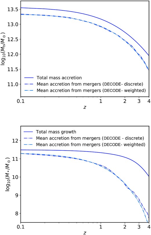
Upper panel: total halo mass accretion history (solid line) along with the comparison between the mergers history of from the discrete and weighted methods (dashed lines). Lower panel: same as upper panel but for galaxy stellar mass.
Similarly to the host dark matter haloes, the bottom panel of Fig. A1 compares the merger contributions to the central galaxy growth computed via the discrete and weighted methods, as labelled, showing again very good agreement between the two methods. We note that this agreement is, as expected, independent of the choice of the input SMHM relation or dynamical friction time-scales, as long as the same parameters are adopted in both methods. We specify once again that, as already noted by G20, each merger tree generated in the discretedecode can show sometimes a merger history that goes beyond the total stellar mass growth of the galaxy, which might seem not physical. This is a direct consequence of the fact that each merger tree in decode is a stochastic realization of the mass functions and probability distributions used as input. However, we test that in the SMHM models that we adopt in this work, the average merger history always lives below the total mass growth and is also fully consistent with what the weighted method predicts, as already shown in Fig. A1. We show in the left-hand panel of Fig. A2 the merger history for our fiducial Model 2 for a galaxy mass bin of |$\sim 10^{11.5} \, \mathrm{M}_\odot$|, where we see that all the single merger histories lie below the total mean mass assembly of the galaxy. On the other hand, in the right-hand panel we show the same results but for Model 2a, where we can clearly see the impact of a lower high-mass end in the SMF leading to a much higher number of mergers, and in many cases not physical as it goes beyond the total growth. The effect of generating an unphysical merger history that, on average, is larger than the total mean stellar mass growth, could be, at least in part, be alleviated by including strong stellar stripping (see e.g. Cattaneo et al. 2011; Smith et al. 2016) and/or stellar mass loss in mergers (e.g. Moster et al. 2018). We will further explore these interesting variants to the model in future work, in combination with the amount of associated star formation our stellar mass accretion tracks predict.
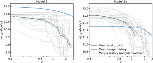
Merger histories of a sample of galaxies with stellar mass at z = 0 of |$\sim 10^{11.5} \, \mathrm{M}_\odot$|, for Models 2 and 2a, as labelled by the panels. The solid blue and grey lines how the average total stellar mass growth and merger history, respectively. The dashed grey lines show the average merger history from the weighted model.
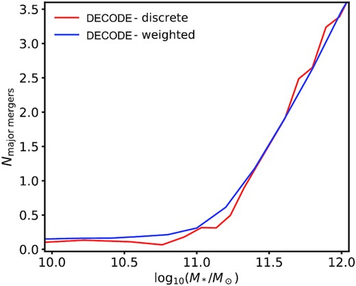
Number of major mergers predicted by the discrete version of decode compared to that computed with the weighted method.
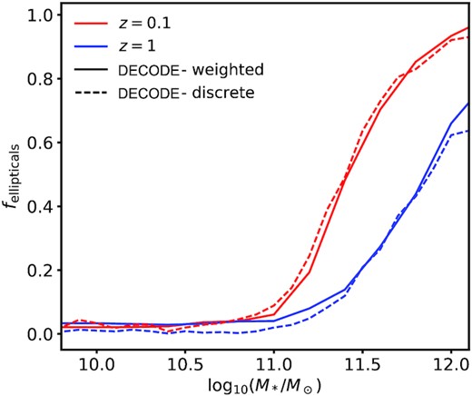
Fraction of ellipticals predicted by the discrete version of decode compared to those computed with the weighted method, for redshifts 0.1 and 1.
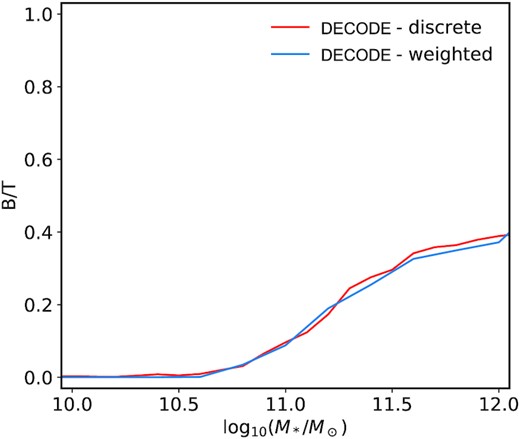
Bulge-to-total ratio predicted by the discrete version of decode compared to that computed with the weighted method for Model BT2.
APPENDIX B: CORRECTION TO THE HALO MASS FUNCTION
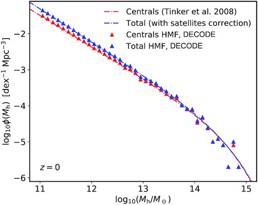
Halo mass function for parent dark matter haloes of Tinker et al. (2008) (red dashed–dotted line) and the total HMF obtained by applying the correction with satellites (blue dashed–dotted line), compared to the mass functions calculated from decode (triangles).
APPENDIX C: HALO AND STELLAR MASS GROWTHS
As already described in Section 3.1, we assign the parent halo with a mean mass assembly history. For the details of how we numerically calculate the latter, we readdress the interested reader to the work of van den Bosch et al. (2014). We show the mean DM accretion for four different values of stellar mass bin (as labelled in the legends) in the left-hand panels of Figs C1 and C2, where we compare with the data from the TNG simulation and EMERGE, respectively. This is a cross-check that the predictions of the TNG simulation and EMERGE are consistent with the mean assembly history that we are employing.
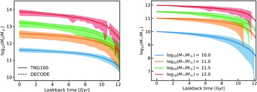
Left-hand panel: halo mass assembly history from the TNG100-1 simulation, for four stellar mass bins at z = 0. Solid lines and shaded areas show the mean and 1σ error from the simulation, and the dashed lines show the accretion history from (van den Bosch et al. 2014) that we adopt in this work. Right-hand panel: total stellar mass growth for the same four mass bins. The dashed lines show the mean galaxy growth computed using the SMHM relation of TNG as input in decode, while the solid lines show the results extracted directly from the TNG data base.
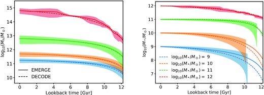
Same as Fig. C1 but for EMERGE.
Similar considerations are valid for the total mean galaxy stellar mass growths. We show in the right-hand panels of Figs C1 and C2 the results predicted by our model decode using as input the SMHM computed from the two simulations, and we compare with the data from the simulations themselves. The stellar mass growth histories for the four masses shown comes out to be consistent within |$\sim 1 \, {\rm dex}$| with TNG and EMERGE.
APPENDIX D: BULGE-TO-TOTAL RATIOS MODELLING
We show in Fig. D1 a comparison of the B/T ratios from different observational data sets. In particular, we compare the MaNGA data (black error bars), described in Section 2.4 and used as a reference for the models in this work, with the SDSS data from Mendel et al. (2014) who selected a subsample of the Simard et al. (2011) catalogue. We also show the B/T ratio of SDSS that we have computed directly from the Simard et al. (2011) catalogue (grey error bars), as well as the predictions of Models 2 from this work (green-dotted and blue-dashed lines). Interestingly, our results for SDSS are not consistent with those from Mendel et al. (2014). Nevertheless, our results discussed in the main text are still valid, irrespective of the exact data set chosen for computing mean B/T ratios. All the three observational B/T ratios show in fact that models based only on mergers, such as our BT1 and BT2 described in Section 4.5, are not sufficient to reproduce the measure B/T ratios, at least at low masses. On the other hand, models that include also disc instabilities perform much better in reproducing the observational data. In summary, all observational B/T data suggest that at low masses some level of disc instabilities is still expected in addition to mergers in order to well describe the evolution of galactic bulges.
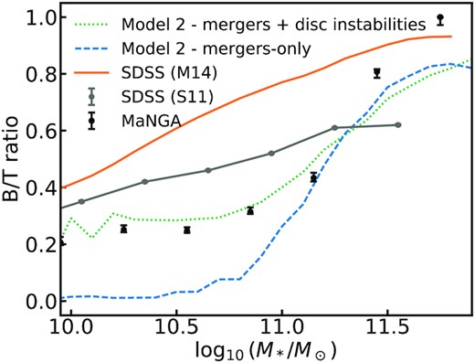
Bulge-to-total ratios as a function of stellar mass from this work compared to different observational samples. The green dotted and blue dashed lines show the Model 2 predictions for the mergers + disc instabilities and mergers-only toy models, respectively. The orange line shows the mean B/T of SDSS using the sample of Mendel et al. (2014), as shown in Devergne et al. (2020). The grey error bars show the SDSS B/T computed using the Simard et al. (2011) catalogue and the black error bars the MaNGA data.
APPENDIX E: SUBHALO ABUNDANCE MATCHING
For completeness, we compare our SMHM relations computed from direct abundance matching between the SMF and the HMF, with the SMHM relation derived from the stellar mass-peak velocity (SMPV) relation (e.g. Guo & White 2014; Chaves-Montero et al. 2016; Contreras et al. 2021; Favole et al. 2022). To this purpose, we first compute the SMPV relation using equation (8), where we input the SMFs of Models 1 and 2, as described in Section 4.1, and we replace the HMF with the peak velocity function. We extract the peak velocity function from the MultiDark simulation (Klypin et al. 2016) at different redshift snapshots. Once the SMPV relation is computed, we calculate the implied SMHM relation and its dispersion at fixed halo mass by using the halo masses competing to each Vpeak in the simulation.
We show the resulting SMHM relation in Figs E1 and E2 at different redshifts (solid blue lines and blue regions), compared with the SMHM relations from decode’s Models 1 and 2, respectively. We see that the relations obtained via the SMPV relation match very well with the SMHM relations from Models 1 and 2. This agreement, on one hand, provides a further validation of our unstripped, surviving subhalo abundance matching technique presented in Section 3.5 and, on the other hand, further highlights that the systematics in the shape and/or redshift evolution of the observed SMF have a strong impact on the resulting mapping between stellar mass and halo mass.
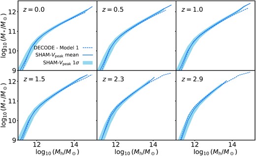
SMHM relation computed via the SHAM technique using the DM Vpeak data from the MultiDark compared to decode at different redshifts. The dashed lines show Model 1 SMHM relation from decode, at different redshifts, as described in Section 4.1. The solid lines and shaded areas show the SMHM relation computed via SHAM with the velocity function using the Model 1 SMF as input and the 1σ dispersion.

Same as Fig. E1 but for Model 2.
