


ABSTRACT
We present new continuum and molecular line data from the ALMA Three-millimeter Observations of Massive Star-forming regions (ATOMS) survey for the two protoclusters, G12.42+0.50 and G19.88−0.53. The 3 mm continuum maps reveal seven cores in each of the two globally contracting protoclusters. These cores satisfy the radius–mass relation and the surface mass density criteria for high-mass star formation. Similar to their natal clumps, the virial analysis of the cores suggests that they are undergoing gravitational collapse (|$\rm \alpha _{vir} \lt \lt 2$|). The clump to core scale fragmentation is investigated and the derived core masses and separations are found to be consistent with thermal Jeans fragmentation. We detect large-scale filamentary structures with velocity gradients and multiple outflows in both regions. Dendrogram analysis of the H13CO+ map identifies several branch and leaf structures with sizes ∼ 0.1 and 0.03 pc, respectively. The supersonic gas motion displayed by the branch structures is in agreement with the Larson power law indicating that the gas kinematics at this spatial scale is driven by turbulence. The transition to transonic/subsonic gas motion is seen to occur at spatial scales of ∼0.1 pc indicating the dissipation of turbulence. In agreement with this, the leaf structures reveal gas motions that deviate from the slope of Larson’s law. From the large-scale converging filaments to the collapsing cores, the gas dynamics in G12.42+0.50 and G19.88−0.53 show scale-dependent dominance of turbulence and gravity and the combination of these two driving mechanisms needs to be invoked to explain massive star formation in the protoclusters.
1 INTRODUCTION
Massive stars (|$M_{\star } \gtrsim 8\, \rm M_{\odot }$|) dictate the dynamical and chemical evolution of the surrounding interstellar medium (ISM) and the galaxy through their mechanical, radiative, and chemical feedback. However, despite the tremendous theoretical, computational, and observational advances in the last decade (Krumholz 2012; Tan et al. 2014; Motte et al. 2018, and references therein), the formation mechanism of high-mass stars, in particular the processes involved in the initial stages, are still not clearly understood. The major issue lies in building a comprehensive multiwavelength data base of this elusive early phase of high-mass stars. Rarity, short evolutionary time-scales, formation in clusters, large distances, and high extinction in embedded environment are the factors that pose observational challenges. In recent years, high-sensitivity and high-resolution observations have rendered several statistical and individual case studies possible with facilities like SMA (e.g. Zhang et al. 2009; Wang et al. 2011; Zhang & Wang 2011; Zhang et al. 2014; Lu et al. 2015; Sanhueza et al. 2017; Pillai et al. 2019; Li et al. 2019b), ALMA (e.g. Sanhueza et al. 2019; Svoboda et al. 2019; Liu et al. 2020a; Barnes et al. 2021; Beltrán et al. 2021; Olguin et al. 2021; Liu et al. 2021, 2022a, b), and CARMA (e.g. Pillai et al. 2011; Sanhueza et al. 2013). Additionally, several surveys like SEDIGISM (Schuller et al. 2017; Yu et al. 2019; Schuller et al. 2021; Yang et al. 2022; Colombo et al. 2022), GLOSTAR (Brunthaler et al. 2021; Nguyen et al. 2021) are also aimed towards addressing various aspects of the formation mechanism and early evolutionary phases of high-mass stars.
In this paper, we present new ALMA data on the massive protoclusters, G12.42+0.50 and G19.88−0.53 (hereafter G12.42 and G19.88, respectively), observed as a part of the ATOMS survey (ALMA Three-millimeter Observations of Massive Star-forming regions survey) (Liu et al. 2020a). This survey provides ALMA Band 3 observations for both continuum and molecular line emission for 146 active star-forming regions (Faúndez et al. 2004) with majority being potential high-mass star-forming regions. The survey is primarily aimed at revealing the spatial distribution of the probed dense gas tracers and deciphering the role of stellar feedback and filaments in the formation of high-mass stars. In the first paper of the ATOMS series, Liu et al. (2020a) present the survey giving details of the configuration used for the continuum and spectral line observations. The authors have also highlighted the major goals of the survey.
G12.42 and G19.88 have been studied by Issac et al. (2019, hereafter Issac19) and Issac et al. (2020, hereafter Issac20), respectively. Both these sources are classified as ‘extended green objects’ (EGOs) by Cyganowski et al. (2008). These are a class of objects believed to be associated with outflows from massive young stellar objects (MYSOs). Issac19 and Issac20 have also provided a brief overview of recent literature on EGOs. G12.42, located at a distance of 2.4 kpc, is catalogued as a ‘possible’ outflow candidate (Cyganowski et al. 2008). Using the Giant Metrewave Radio Telescope (GMRT) radio continuum observations at 610 and 1390 MHz, Issac19 suggest the co-existence of an UC H ii region and an ionized jet that are likely powered by the MYSO, IRAS 18079-1756. The ionized jet inference is strongly supported by near-infrared (NIR) spectroscopic observations presented by these authors where the detection of the shock-excited lines of |$\rm H_2$| and [Fe ii] are reported. Additionally, these authors show that the observed radio emission is located at the centroid position of the detected wide-angle bipolar CO outflow which also supports the radio thermal jet scenario (Anglada 1996; Rodriguez 1997). The other protocluster, G19.88, located at a distance of 3.31 kpc, is catalogued as a ‘likely’ outflow candidate and associated with IRAS 18264-1152 (Cyganowski et al. 2008). Issac20 present GMRT observations at the frequencies mentioned above. Their study reveals the presence of an ionized jet which is deciphered to be associated with a massive, dense, and hot ALMA 2.7 mm core powering a bipolar CO outflow. In combination with the ALMA Band 3 and 7 continuum and line emission data, G19.88 is understood to be an active protocluster with high-mass star-forming cores in various evolutionary phases. Liu et al. (2021) (the third paper in the ATOMS series) catalogued the high mass star-forming cores associated with G12.42 as ‘unknown cores,’ as they do not enshroud hyper/ultra compact H ii regions and the spectra lack evidence of complex organic molecules (COM) (e.g. CH3OCHO, CH3CHO, CH3OH, C2H5CN). Whereas, G19.88 is listed as ‘pure w-cHMC,’ which contains high-mass cores with relatively low levels of COM richness and not associated with hyper/ultra compact H ii regions. The details of the two protoclusters are compiled in Table 1. In this paper, we use the data from the ATOMS survey to conduct a detailed study of the detected 3 mm cores and focus on a multispectral line study to understand the kinematics and gas dynamics of the regions associated with G12.42 and G19.88 from clump to core scale. The paper is organized as follows. Section 2 discusses the ALMA observations carried out as a part of the ATOMS survey and the complementary archival data used in this study. Results obtained from the continuum and molecular line analysis are presented in Section 3. Sections 4 and 5 address the gravitational stability and fragmentation scenario of the clumps. Section 6 delves into detailed analysis and discussion of multiscale gas kinematics that includes the large-scale filamentary structures, small-scale density structures, and the cores. The interplay between gravity and turbulence in driving star formation in the two protoclusters is explored in Section 7. Section 8 summarizes the results and subsequent interpretation of this study.
Basic information of the protoclusters.
| Source | Coordinatesa | Distance | |$\rm V_{LSR}$| | |
|---|---|---|---|---|
| RA(J2000) | DEC(J2000) | (kpc) | (|$\rm km\, s^{-1}$|) | |
| G12.42+0.50 | 18:10:50.6 | −17.55.47.2 | 2.4b | 18.3c |
| G19.88−0.53 | 18:29:14.3 | −11.50.27.0 | 3.3d | 44.0e |
| Source | Coordinatesa | Distance | |$\rm V_{LSR}$| | |
|---|---|---|---|---|
| RA(J2000) | DEC(J2000) | (kpc) | (|$\rm km\, s^{-1}$|) | |
| G12.42+0.50 | 18:10:50.6 | −17.55.47.2 | 2.4b | 18.3c |
| G19.88−0.53 | 18:29:14.3 | −11.50.27.0 | 3.3d | 44.0e |
2 OBSERVATIONS AND ARCHIVAL DATA
2.1 ALMA observations
ALMA data from the ATOMS survey (Project ID: 2019.1.00685; PI:Tie Liu) are used for studying the G12.42 and G19.88 complexes. The 12-m array observations of both complexes were conducted on -2019 November 1. The ACA observations of the same were conducted on the 2019 November 2 and 3, with two executions. On-source integration times on each source for 12-m array and ACA array are ∼3 and 8 min, respectively. Calibration of the 12-m array data and ACA data were done separately using the Common Astronomy Software Applications (casa) package version 5.6 (McMullin et al. 2007). Subsequent to this, the visibility data were also combined and imaged in casa to recover the very extended emission that is missed in the 12-m array observations. All images used in our analysis are primary beam corrected. The high-resolution 3 mm (∼99.93 GHz) continuum map, with beam size of 1.75 arcsec × 1.3 arcsec and rms noise of 0.2 |$\rm mJy\, beam^{-1}$|, is constructed using data from line-free spectral channels. In addition to the continuum data, in the ATOMS survey eight spectral windows (SPWs) were configured to sample eleven major molecular lines that include dense gas tracers (e.g. J = 1−0 of HCO+, HCN, and their isotopes), hot core tracers (e.g. CH3OH, HC3N), shock tracers (e.g. SiO, SO), and ionized gas tracers (|$\rm H_{40\alpha }$|). The species name, transitions, rest frequencies, and basic parameters (e.g. critical density and upper level energy) of these molecular lines are summarized in table 2 of Liu et al. (2020a). Details (angular resolution, linear resolution, maximum recoverable scale (MRS), and the rms level) of the ATOMS data used in this study are compiled in Table 2. More details can be found in table 1 of Liu et al. (2020a). Continuum maps and the velocity integrated intensity maps of all the molecules observed in ATOMS survey are shown in Figs 1 and 2.
![Continuum (3 mm) and moment zero maps of all the molecular transitions observed towards G12.42+0.50 in the ATOMS survey are shown. The continuum map is generated from the high-resolution 12-m data only while the line maps are from the 7-m + 12-m combined data. The maps are integrated over the velocity range [−32, 58] $\rm km\, s^{-1}$ which is approximately $\rm V_{LSR} \pm 50\, \rm km\, s^{-1}$ and incorporates all emission features. This enables easy comparison between various molecular lines with the same integrated velocity range. The colour bar indicates the flux scale in $\rm Jy\, beam^{-1}\, km\, s^{-1}$ for moment zero maps and $\rm Jy\, beam^{-1}$ for the continuum map. The beam size is indicated at the bottom left in each panel. The red ellipses represent the identified cores (see Section 3.1).](https://oup.silverchair-cdn.com/oup/backfile/Content_public/Journal/mnras/516/2/10.1093_mnras_stac2353/1/m_stac2353fig1.jpeg?Expires=1750467463&Signature=GjWjibXq83rAOvHQQ-tSyABuFHmGjDo3~ScLR8m7XfMjknfW7bD23c0nKnfnCrIrSMajPhuPSZVLr1T5LBOADrnJ4VyArArOKhJ8qvxtkT1~b6A9fOyIvPPrF66D1ZkPGrQ3Cnc0avkm3YsSbQ8o1QMBe06rgiHGvPISUy8XEvlX~Scf5TA3UfzL9oQZazgmuGRIotdNsT6Ke7TWOU23v6XTe6QciPHwA2BjpFWiruZCiE7WzXOclpO2lMQEthpZSmGdF5zKVDsInkW9f~1hSMNRtB-9tAvh-Zuf6hbUBba3~raxbT4~eg3ieqxThYBlW4XldYgNwYmWp7~zUlotCQ__&Key-Pair-Id=APKAIE5G5CRDK6RD3PGA)
Continuum (3 mm) and moment zero maps of all the molecular transitions observed towards G12.42+0.50 in the ATOMS survey are shown. The continuum map is generated from the high-resolution 12-m data only while the line maps are from the 7-m + 12-m combined data. The maps are integrated over the velocity range [−32, 58] |$\rm km\, s^{-1}$| which is approximately |$\rm V_{LSR} \pm 50\, \rm km\, s^{-1}$| and incorporates all emission features. This enables easy comparison between various molecular lines with the same integrated velocity range. The colour bar indicates the flux scale in |$\rm Jy\, beam^{-1}\, km\, s^{-1}$| for moment zero maps and |$\rm Jy\, beam^{-1}$| for the continuum map. The beam size is indicated at the bottom left in each panel. The red ellipses represent the identified cores (see Section 3.1).
Details of ALMA data.
| Continuum data (12-m array): | ||
| Source | G12.42+0.50 | G19.88−0.53 |
| Angular resolution | 1.75 arcsec × 1.3 arcsec | 0.46 arcsec × 0.28 arcsec |
| Linear resolution (pc × pc) | 0.020 × 0.015 | 0.007 × 0.004 |
| rms noise (|$\rm mJy\, beam^{-1}$|) | 0.2 | 0.12 |
| Maximum recoverable scale (MRS) | 18.3 arcsec | 5.2 arcsec |
| Line Data (12-m + 7-m arrays): | ||
| Transition | |$\rm H^{13}CO^+$| (1–0)/ | |$\rm HCO^+$| (1–0) |
| SiO (2–1) | ||
| Angular resolution | 2.5 arcsec × 2.0 arcsec | 2.4 arcsec × 1.9 arcsec |
| Linear resolution (pc × pc) | 0.029 × 0.023a | 0.028 × 0.022a |
| 0.040 × 0.032b | 0.038 × 0.030b | |
| Velocity resolution (|$\rm km\, s^{-1}$|) | 0.2 | 0.1 |
| rms noise (|$\rm mJy\, beam^{-1}$|) | 8 | 12 |
| Maximum recoverable scale (MRS) | 76.2 arcsec | 76.2 arcsec |
Note: a and b are the linear resolutions corresponding to G12.42+0.50 and G19.88−0.53, respectively.
2.2 Archival ALMA continuum data
Continuum emission towards G19.88 complex at 2.7 mm (∼ 111.0 GHz) was retrieved from the ALMA archives (Project ID: 2017.1.00377.S; PI:S. Leurini). Observations were conducted in the session 2017–2018. These high-resolution ALMA observations were obtained with the 12-m array in the FDM Spectral Mode. The minimum baselines, maximum baselines, and MRS in this observation are 15.07 m, 2386.1 m, and 5.2 arcsec, respectively. The 2.7 mm continuum map, with beam size of 0.46 arcsec × 0.28 arcsec and rms noise of 0.12 |$\rm mJy\, beam^{-1}$|, is used to identify and study the cores associated with G19.88. Details of the ALMA archival data used in this study are listed in Table 2.
2.3 Spitzer archival data
To investigate the morphology of the mid-infrared (MIR) emission in regions associated with G12.42+0.50 and G19.888−0.53, we obtained MIR images from the archives of the Galactic Legacy Infrared Midplane Survey Extraordinaire (GLIMPSE) survey of the Spitzer Space Telescope. The Infrared Array Camera (IRAC) mounted on the Spitzer Space Telescope is capable of simultaneous broad-band imaging at 3.6, 4.5, 5.8, and 8.0 |$\, \mu$|m (Fazio et al. 2004). We retrieved images having an angular resolution of ≲2 arcsec with a pixel size of ∼0.6 arcsec in three IRAC bands (3.6, 4.5, and 8.0 |$\, \mu$|m) (Benjamin et al. 2003).
2.4 JCMT archival data
The molecular line data for |$\rm {}^{13}CO$| (3–2) transition were obtained from the archives of James Clerk Maxwell Telescope (JCMT) to investigate the filamentary morphology of the star-forming region associated with G12.42. The velocity structure of filaments using JCMT |$\rm {}^{12}CO$| (3–2) transition presented in Issac19 was utilized to investigate the gas kinematics. Heterodyne Array Receiver Program (HARP) mounted on the 15 m JCMT telescope comprises of 16 detectors laid out on a 4 × 4 grid, with an on-sky beam separation of 30 arcsec. The molecular line observation for |$\rm {}^{13}CO$| (3–2) was carried out using HARP at a rest frequency of ∼330.6 GHz. The beam size of JCMT at 345 GHz is 14 arcsec (Buckle et al. 2009). |$\rm {}^{13}CO$| (3–2) and |$\rm {}^{12}CO$| (3–2) data have a channel width of 0.055 and 0.42|$\, \rm km\, s^{-1}$|, with an rms level per channel of 1.9 and 1.0 K, respectively.
3 RESULTS
3.1 Continuum emission
We use the observed 3 mm continuum emission maps to identify and study compact cores in the regions associated with the protoclusters under study. The derived properties of these cores enable us to understand their nature and formation. The lower left-hand panel of Figs 1 and 2 present the 3 mm continuum map for the entire field of view of the ATOMS survey. An enlarged view of the extended continuum emission morphology and the identified cores in G12.42 and G19.88 are shown in Fig. 3.
![Same as Fig. 1, but for the protocluster G19.88−0.53. The maps are integrated over the velocity range [−21, 109] $\rm km\, s^{-1}$ which is approximately $\rm V_{LSR} \pm 65\, \rm km\, s^{-1}$.](https://oup.silverchair-cdn.com/oup/backfile/Content_public/Journal/mnras/516/2/10.1093_mnras_stac2353/1/m_stac2353fig2.jpeg?Expires=1750467463&Signature=vbo6fngtZyphr8jKx0wfE~8eaglTTcstN9o2O13d6MbvKX4QmTMN73bCU1oSPKwMsBn6xsF2v4qDt4CNCcmoFAGBA1ex5ssw~fp4UZ9tfRDyo-FIrnEJ7aJPWk-diBW7i8EAZOiY7mEYGry0SeR1jTii1U6qK-M5tfOESWHWuiyHYOhxld9RULf10S810yDRFO3mSaEAB77Ab3G22PUJB73l0JuK40Im43mD26wtOD-UcDZqAbw-WvY0t0amR-ed6zxGVT1Ue~MEDCpKEc6-O38jtYAe0EkHtM4CKTlD5xrROUpd0wRcN1xgL-yevIOiidJEx-prOPG-ETIEcLMM-g__&Key-Pair-Id=APKAIE5G5CRDK6RD3PGA)
Same as Fig. 1, but for the protocluster G19.88−0.53. The maps are integrated over the velocity range [−21, 109] |$\rm km\, s^{-1}$| which is approximately |$\rm V_{LSR} \pm 65\, \rm km\, s^{-1}$|.
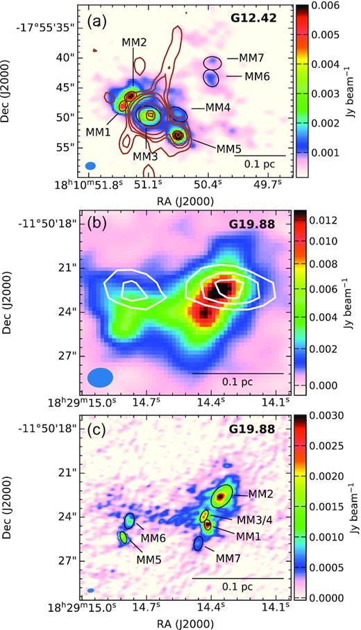
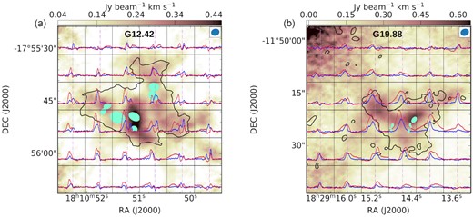
(a) 3 mm continuum map of the region associated with G12.42+0.50 obtained using 12-m array data from ATOMS is shown in colour scale. Core apertures acquired using casa-imfit are shown in black ellipses. The overlaid contours showing the radio emission at 1390 MHz (beam size is 3.0 arcsec × 2.4 arcsec) with contour levels at 3, 6, 9, 18, 63, 150, and 172 times σ (σ ∼ 29.7 |$\rm \mu Jy\, beam^{-1}$|) are from Issac19. (b) Same as figure (a) but for G19.88−0.53. The overlaid contours showing the radio emission at 1390 MHz (beam size is 4.3 arcsec × 2.7 arcsec) with contour levels at 3, 4, 5, and 6 times σ (σ ∼ 45 |$\rm \mu Jy\, beam^{-1}$|) are from Issac20. (c) The colour scale shows the 2.7 mm continuum emission of the region associated with G19.88−0.53 obtained using 12-m array data from the ALMA archive. The black ellipses represent the core apertures acquired using casa-imfit. The beam of the continuum maps are indicated at the bottom left in each figure.
3.1.1 Core identification
Cores in both complexes have been identified in ATOMS III paper (Liu et al. 2021). These authors have also derived the physical parameters. In addition to this, compact cores in G12.42 (SMA; 1.1 mm) and G19.88 (ALMA; 2.7 mm) have been analysed in Issac19 and Issac20, respectively. Liu et al. (2021) have detected the most prominent cores (four in G12.42 and two in G19.88) in these protoclusters. Issac19 have identified three SMA cores in G12.42 and Issac20 have detected six ALMA cores in G19.88. Based on these results and a careful visual inspection of the ATOMS continuum map, we are prompted to revisit the core identification before proceeding for further analysis. The 3 mm continuum emission towards G12.42 and G19.88 observed with the 12-m array are shown in Figs 3(a) and (b). For core detection in G19.88, we use available higher resolution data at 2.7 mm from the ALMA archives. This is the same data set used in Issac20 and the map is shown in Fig. 3(c).
Following the approach introduced in Li et al. (2020a) and outlined in Liu et al. (2020a, 2021, 2022a), cores are extracted by utilizing the astrodendro1 package and the casa imfit task. The dendrogram technique (Rosolowsky et al. 2008) decomposes the emission into a hierarchy of substructures, providing a good representation of the topography of the star-forming region. Dense structures (leaves in the terminology of the algorithm) which are not further divisible into smaller structures are considered as potential candidates to become star-forming cores. To identify the leaves, the following parameters are used: (i) |$min\_value = 3 \sigma$|, which is the minimum threshold to be considered in the data set and σ is the rms noise; (ii) |$min\_delta = \sigma$|, the default value in the algorithm which determines how significant a leaf has to be in order to be considered an independent entity; (iii) |$min\_npix = N$| pixels, which is the minimum number of pixels needed for a leaf. To ensure cores are resolvable, N is chosen to be equivalent to the synthesized beam area in units of pixel. The algorithm returns several parameters (i.e. position of the centre, major and minor axis sizes, position angle) of the identified cores.
Next, the casa imfit task is used with the dendrogram parameter outputs as the corresponding initial estimates of the fit parameters. During the fitting process none of the parameters are fixed. A bounding box is used, the size of which is defined based on the retrieved aperture of the leaves in the dendrogram analysis. We have not considered background subtraction as large-scale extended emission, which can be regarded as the background component, is already filtered-out in the interferometric data. The derived physical parameters, which includes the peak position, deconvolved major and minor sizes (FWHMmaj, FWHMmin), position angle (PA), peak intensity (Fpeak), and integrated flux density (Fint) are listed in Tables 3 and 4 for G12.42 and G19.88, respectively. In order to avoid inclusion of spurious cores in our analysis, we retain only those satisfying, Fpeak > 5σ. Further, we also reject cores with poorly fitted shapes by visual inspection of the continuum map overlaid with the identified leaf structures. These usually appear either as filamentary structures or diffuse emission features with an aspect ratio of more than three, between the length of the major and minor axis. The identified cores are overlaid in Figs 3(a) and (c).
Parameters of detected cores in protocluster G12.42+0.50, using data from 12-m array at 3 mm.
| Core | Peak position | Deconvolved size | PA | Fint | Fpeak | Reff | Rcore | |$M^{\rm a}_{\rm core}$| | Σ | ||
|---|---|---|---|---|---|---|---|---|---|---|---|
| RA(J2000) | DEC(J2000) | Major (arcsec) | Minor (arcsec) | deg | |$\rm mJy$| | |$\rm mJy\, beam^{-1}$| | (arcsec) | 10−2 pc | (|$\rm M_\odot$|) | g cm−2 | |
| MM1 | 18:10:51.39 | −17.55.48.04 | 1.84 | 1.31 | 156 | 10.9 | 5.2 | 0.8 | 0.9 | 24.0 | 19.5 |
| MM2 | 18:10:51.31 | −17.55.46.37 | 2.13 | 1.50 | 116 | 14.9 | 6.3 | 0.9 | 1.0 | 32.9 | 20.2 |
| MM3 | 18:10:51.10 | −17.55.49.60 | 4.31 | 3.21 | 72 | 22.2 | 3.2 | 1.9 | 2.2 | 48.9 | 6.9 |
| MM4 | 18:10:50.75 | −17.55.49.40 | 3.4 | 2.17 | 61 | 6.8 | 1.6 | 1.4 | 1.6 | 15.0 | 4.0 |
| MM5 | 18:10:50.75 | −17.55.52.89 | 1.79 | 1.48 | 69 | 14.9 | 7.0 | 0.8 | 1.0 | 32.8 | 23.9 |
| MM6 | 18:10:50.58 | −17.55.54.50 | 2.96 | 2.39 | 30 | 4.6 | 1.1 | 1.3 | 1.6 | 10.1 | 2.8 |
| MM7 | 18:10:50.36 | −17.55.43.37 | 2.97 | 2.22 | 86 | 3.7 | 0.9 | 1.3 | 1.5 | 8.1 | 2.4 |
Note: a Temperature of 25 K is considered to calculate the mass of all the cores.
Parameters of detected cores in the protocluster G19.88−0.53, using 2.7 mm data.
| Core | Peak position | Deconvolved size | PA | Fint | Fpeak | Reff | Rcore | Mcore | Ta | Σ | ||
|---|---|---|---|---|---|---|---|---|---|---|---|---|
| RA(J2000) | DEC(J2000) | Major (arcsec) | Minor (arcsec) | deg | |$\rm mJy$| | |$\rm mJy\, beam^{-1}$| | (arcsec) | 10−2 pc | |$\rm M_\odot$| | K | g cm−2 | |
| MM1 | 18:29:14.41 | −11.50.24.52 | 0.70 | 0.45 | 8 | 11.3 | 3.0 | 0.3 | 0.5 | 9.3 | 82.7 | 35.7 |
| MM2 | 18:29:14.35 | −11.50.22.58 | 1.81 | 1.16 | 140 | 39.0 | 2.2 | 0.7 | 1.1 | 22.7 | 115.9 | 13.1 |
| MM3c | 18:29:14.43 | −11.50.24.10 | 0.91 | 0.44 | 155 | 10.5 | 2.3 | 0.3 | 0.5 | 8.7 | 82.7 | 26.1 |
| MM4c | 18:29:14.43 | −11.50.23.93 | 0.91 | 0.44 | 155 | 10.5 | 2.3 | 0.3 | 0.5 | 8.7 | 82.7 | 26.1 |
| MM5 | 18:29:14.80 | −11.50.25.37 | 0.84 | 0.41 | 18 | 6.3 | 1.5 | 0.3 | 0.5 | 9.4 | 47.2 | 32.8 |
| MM6 | 18:29:14.78 | −11.50.24.26 | 1.09 | 0.65 | 167 | 6.80 | 1.0 | 0.4 | 0.7 | 10.1 | 47.2 | 17.0 |
| MM7 | 18:29:14.46 | −11.50.25.78 | 0.96 | 0.59 | 167 | 4.0 | 0.7 | 0.4 | 0.6 | 3.3 | 82.7 | 5.8 |
Note: a Temperature corresponding to each core is taken from Issac20, c MM3 and MM4 are unresolved in the map, hence the quoted parameters refer to the combined region enclosing both the cores.
For G12.42, we identify seven cores, MM1–MM7. It is to be noted that in case of this source, cores MM1 and MM2 which are named SMA1 and SMA2 in Issac19, are manually fitted using casa imfit since the dendrogram algorithm resolved it into a single leaf though two distinct cores are seen visually. For G19.88, we also identify seven cores, MM1–MM7. In their analysis, Issac20, had visually identified six cores and used the casa imfit task to determine the parameters. For the common cores, the overall core extraction carried out in this work agrees well with Issac19, Issac20, and Liu et al. (2021).
To address the concern of ‘missing flux’ in high-resolution interferometric observations, we compare the retrieved deconvolved sizes of the compact cores with that of the MRS of the two data sets used. Considering the 12-m data used for core identification in G12.42, the deconvolved sizes of the cores lie in the range, 1.6–3.7 arcsec, which is much smaller (≲ 20 per cent) than the MRS of ∼18 arcsec. Further, comparing the retrieved fluxes from the 12-m and the combined data, Liu et al. (2021, 2022a) discuss that the uncertainties on the estimated flux due to ‘missing flux’ is not significant. In case of G19.88, we have used the higher resolution archival ALMA data to detect the cores where the MRS quoted is ∼5 arcsec and the retrieved sizes lie in the range, 0.6–1.5 arcsec which are again smaller than the MRS. Nevertheless, for the largest core (MM2), we compare the flux retrieved with that from the 12-m ATOMS data and found them to be equal. This indicates that the estimated parameters of the compact cores in G12.42 and G19.88 are not significantly affected and only the diffuse, larger scale emission between clumps could have been filtered out.
The 3 mm continuum emission can have contributions from both thermal dust emission and free–free emission from ionized gas. Based on the lack of |$\rm H_{40\alpha }$| radio recombination line emission observed in the ATOMS survey, Liu et al. (2021) classified these prominent cores in G12.42 and G19.88 as ones without association with HC or UC H ii regions. However, weak centimetre radio emission, interpreted as possible thermal jets, has been detected in cores MM3 and MM5 in G12.42 (Issac19) and core MM2 in G19.88 (Issac20). The radio emission is shown as contours in Figs 3(a) and (b). Free–free emission from radio jets become optically thin for frequencies greater than the turnover frequency and the spectral index becomes −0.1 (Anglada, Rodríguez & Carrasco-González 2018). Without the information of the turnover frequency either from observed radio spectral energy distribution or from theoretical modelling of the jet emission for the three cores discussed above, it is difficult to estimate the contribution of free–free emission at 3 mm. For a crude estimate, we assume the highest frequency data available (5 GHz for G12.42 and 23 GHz for G19.88) as the turnover frequency and extrapolate the measured fluxes to 3 mm (100 GHz) assuming an optically thin spectral index of −0.1. This is reasonably consistent with Anglada et al. (2018) who have adopted a lower limit of 10 GHz for the turnover frequency to estimate the physical parameters of the radio emission from ionized jets.
For G12.42, 5 GHz continuum flux density is taken from Issac19 and for G19.88, 23 GHz flux density is taken from Zapata et al. (2006). Extrapolating gives 20 per cent and 5 per cent contribution from ionized gas emission to the 3 mm flux estimate of cores MM3 and MM5, respectively, of G12.42 and 2 per cent contribution to the 2.7 mm flux estimate for core MM2 of G19.88. For core MM3 of G12.42, the contribution from free–free emission may result in the mass (see the next section) being overestimated by a factor of 1.3.
In summary, free–free emission does not significantly affect the continuum flux-derived parameter estimates (e.g. mass, and density) of the cores studied here.
3.1.2 Physical properties of detected cores
3.2 Molecular line emission from combined ALMA 12-m array and ACA data
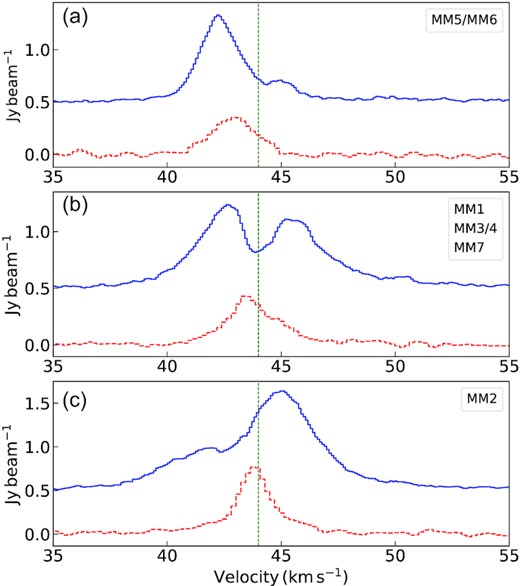
Detailed kinematic information is key to understanding the gas dynamics in the star-forming clouds which enables us to probe the star-formation scenario therein. The velocity integrated intensity (moment zero) maps of the molecular transitions observed for these sources in the ATOMS survey, are shown in Figs 1 and 2 illustrating the spatial distribution of these species in the two star-forming regions. Multipeak features are seen in most molecular transitions. There is no |$\rm H_{\alpha }$| emission detected. For G12.42, |$\rm H^{13}CO^{+}$| map reveals interesting filamentary morphology. This transition is a good tracer of filamentary clouds which is illustrated in the detection of a complex network of narrow filamentary structures toward a massive infrared dark cloud, NGC 6334S (Li et al. 2022). In both star-forming complexes (G12.42 and G19.88), maps of the outflow/shock tracers (SiO, SO, and CS) reveal elongated and collimated structures. To investigate the global and the core kinematics of G12.42 and G19.88, we have used the spectral line data of H13CO+, HCO+, and SiO transitions. In Figs 4 and 5, we present the clump-averaged spectra, extracted over the region enclosed within the 3σ level of the continuum emission for G12.42 and G19.88. The systemic velocity of 18.3 |$\rm km\, s^{-1}$| (Yu & Wang 2015) and 44.0 |$\rm km\, s^{-1}$| (Beuther et al. 2002b; Qiu et al. 2007) for G12.42 and G19.88, respectively, are shown as green dashed vertical lines in the plots. As seen in Fig. 4(a), the line profiles of HCO+ (1–0) and H13CO+ (1–0) display double peaked, blue-skewed profiles being more prominent in the optically thick transition of HCO+ (1–0). The dip in the line profile for H13CO+ (1–0) is at the systemic velocity (Fig. 4a), while that for HCO+ (1–0) is redward of it. Extended line wings, seen prominently here in HCO+, are the signature of outflows. The SiO spectra are shown in Fig. 5(a) where the spectrum fits to a combination of a broad and a narrow Gaussian components. The nature of this profile will be further discussed in Section 6.3.
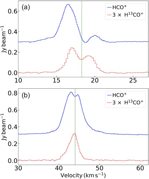
Clump-averaged spectra of the molecular lines (H13CO+, HCO+) detected towards G12.42+0.50 and G19.88-0.53 using combined 12-m + 7-m data are shown in panel (a) and (b), respectively. The spectra are averaged over a region enclosed by the 3σ contour continuum emission for G12.42 and G19.88, respectively. HCO+ spectra shown in blue (solid) are vertically offset by 0.3 |$\rm Jy\, beam^{-1}$| and H13CO+ spectra shown in red (dashed) are scaled-up by a factor of 3 in both the panels. The vertical dashed line in each panel marks the LSR velocity of 18.3 and 44.0 |$\, \rm km\, s^{-1}$| for G12.42 and G19.88, respectively.
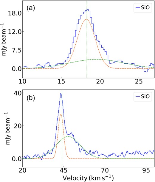
Clump-averaged spectra of SiO (2–1) detected towards G12.42+0.50 and G19.88-0.53 using combined 12-m + 7-m data are shown in panels (a) and (b), respectively. The spectra are averaged over a region enclosed by the 3σ contour continuum emission for G12.42 and G19.88, respectively. The spectra are boxcar smoothed by four channels resulting in a velocity resolution of 0.84|$\, \rm km\, s^{-1}$|. The orange and green dashed lines indicate the decomposed components of SiO (2–1) line. The vertical dashed line in each panel marks the LSR velocity of 18.3 and 44.0 |$\, \rm km\, s^{-1}$| for G12.42 and G19.88, respectively.
For G19.88, the relatively optically thin H13CO+ (1–0) spectrum shows a single peak profile with the peak consistent with the LSR velocity, whereas the HCO+ spectrum of G19.88 is double-peaked and marginally blue-skewed with the dip at the systemic velocity where the single component |$\rm H^{13}CO^{+}$| line peaks (refer Fig. 4b). Outflow wings are seen in both HCO+ and |$\rm H^{13}CO^{+}$| transitions. The SiO spectrum (Fig. 5b) also displays the double-Gaussian profile as discussed above.
To probe the gas kinematics at the core level, we extract the |$\rm HCO^+$| and |$\rm H^{13}CO^+$| spectra over circular areas of diameter ∼2.5 arcsec (typical beam size of the molecular line data) that adequately covers the detected core apertures in both complexes. For G12.42, H13CO+ and HCO+ spectra extracted over an area enclosing MM1, MM2, MM3, MM4, MM5, MM6, and MM7 are shown in Figs 6(a)–(g), respectively. The H13CO+ spectra covering cores MM1, MM2, and MM3 display single peaked profiles, whereas the HCO+ profiles are blue-skewed, double-peaked with the dip consistent with the peak of H13CO+ (1-0) emission. Prominent blue line wings are discernible in the HCO+ line profiles of MM1 and MM2. For MM3, the blue component is relatively broader, and the outflow wing is marginally visible. Spectra for the other cores show complex, double-peaked profiles. For the cores MM6 and MM7, the two observed components of HCO+ and H13CO+ do not peak at the same velocity. The peak of H13CO+ lies in between and close to the dip seen in the HCO+ spectra. This could be a possible infall signature. Given the beam size (∼2.5 arcsec) of the molecular line data, it is difficult to extract the spectra over individual cores in G19.88 as the regions would overlap. Hence, for this protocluster, we extract H13CO+ and HCO+ spectra over apertures covering MM5-MM6, MM1-MM3-MM4, and MM2 which are shown in Figs 7(a), (b), and (c), respectively. In the spectra covering cores MM5 and MM6, the HCO+ line profile seem to be a blue-skewed, double-profile though the red component is not very prominent. The H13CO+ spectrum shows single profile with a bump on the red side. The possibility of this being another component cannot be ruled out. The spectrum for the region covering MM1-MM3-MM4-MM7 shows a blue-skewed, double-peaked HCO+ line with a single peaked H13CO+ profile, the peak of which coincides with the dip seen in the other and matches with the systemic velocity. The line profiles for MM2 are single peaked. All regions show strong signatures of outflow wings, being most pronounced for MM2. Higher resolution molecular line data are essential to probe the kinematics of the individual cores in G19.88.
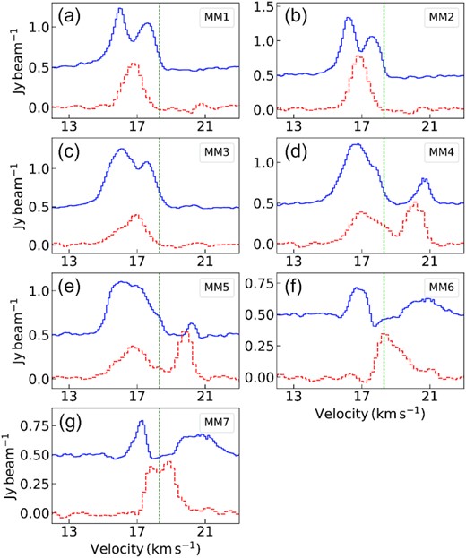
HCO+ and H13CO+ spectra taken towards the cores associated with G12.42+0.50 are shown in blue (solid) and red (dashed) in each panel, respectively using combined 12-m + 7-m data. HCO+ spectra are vertically offset by 0.5 |$\rm Jy\, beam^{-1}$| and H13CO+ spectra are scaled-up by a factor of 3 in all the panels. The vertical dashed lines mark the LSR velocity VLSR = 18.3 |$\, \rm km\, s^{-1}$|. Plots (a)–(g) present the core-averaged spectra covering (a) MM1, (b) MM2, (c) MM3, (d) MM4, (e) MM5, (f) MM6, and (g) MM7, respectively.
HCO+ and H13CO+ spectra taken towards the cores associated with G19.88–0.53 are shown in blue (solid) and red (dashed) in each panel, respectively using combined 12-m + 7-m data. HCO+ spectra are vertically offset by 0.5 |$\rm Jy\, beam^{-1}$| and H13CO+ spectra are scaled-up by a factor of 3 in all the panels. The vertical dashed lines mark the LSR velocity VLSR = 44.0|$\, \rm km\, s^{-1}$|. Plots (a)–(c) present the spectra averaged over cores (a) MM5 and MM6, (b) MM1, MM3/MM4, and MM7 (c) MM2, respectively.
4 GRAVITATIONAL STABILITY AND GLOBAL COLLAPSE SCENARIO
3 mm clump parameters.
| Clump | Line width (ΔV) | Radius (r) | Mcl-3mm | Mvir | αvir |
|---|---|---|---|---|---|
| |$\rm km\, s^{-1}$| | (pc) | (|$\rm M_{\odot }$|) | (|$\rm M_{\odot }$|) | ||
| G12.42 | 1.8 | 0.3 | 478 | 126 | 0.3 |
| G19.88 | 3.0 | 0.4 | 1078 | 475 | 0.4 |
| Clump | Line width (ΔV) | Radius (r) | Mcl-3mm | Mvir | αvir |
|---|---|---|---|---|---|
| |$\rm km\, s^{-1}$| | (pc) | (|$\rm M_{\odot }$|) | (|$\rm M_{\odot }$|) | ||
| G12.42 | 1.8 | 0.3 | 478 | 126 | 0.3 |
| G19.88 | 3.0 | 0.4 | 1078 | 475 | 0.4 |
The virial parameter enables us to understand the stability of the protostellar clumps. Clumps are gravitationally bound and unstable to collapse if they are supercritical with αvir << αcr, αcr being a critical virial parameter. If we consider non-magnetized clumps then αcr ∼ 2 whereas, αcr << 2 is possible in the presence of strong magnetic support. For both the protostellar clumps we estimate αvir ∼ 0.3–0.4. The actual values could be still lower since the presence of infall/outflow in these regions would result in broadened line profiles thus leading to overestimation of the parameter. Such low values of the virial parameter are generally observed towards high-mass star-forming clumps (e.g. Pillai et al. 2011; Kauffmann et al. 2013; Contreras et al. 2016; Tang et al. 2019). For G12.42 and G19.88, these estimated low values indicate that these clumps are supercritical and are undergoing strong gravitational collapse if no other supporting mechanism (e.g. magnetic field) exists. Magnetic field effects, if present, have not been considered in the estimation of αvir as no magnetic field study is available for these protoclusters in literature. Magnetic field plays an important role and if there exists additional magnetic support then including the Alfvén velocity term would give a larger value for αvir (see equation 9 of Tang et al. 2019).
Several studies have used optically thick molecular line transitions to decipher global gas dynamics in star-forming clumps (e.g. Klaassen et al. 2012; He et al. 2015). HCO+ is an excellent dense gas tracer that is commonly used to reveal global infall signatures. This constitutes a double-peaked, blue asymmetrical line profile with a self-absorption dip at the systemic velocity. To rule out multiple components along the line of sight, for a bona fide infall candidate, the relatively less optically thick isotopologue, H13CO+, is also required to be single peaked coinciding with the above self-absorption dip. G12.42 has been identified as an infall candidate by He et al. (2015) based on the line profiles as discussed above. This inference was also confirmed by Issac19. Both these studies are based on single dish MALT90 molecular line data. Issac19 used the optically thin H13CO+(1–0) and the optically thick HCO+(1–0) lines to trace infall. Using similar approach and another transition (|$\rm \mathit{ J} = 4 - 3$|) of the same pair of lines, no infall is inferred for the G19.88 clump (Klaassen, Testi & Beuther 2012). This is consistent with the conclusion arrived at by another study conducted by Jin et al. (2016) using the HCN and HNC molecular line transitions. Both these results are again based on single dish observations.
We revisit the infall analysis with high-resolution ATOMS-ALMA observation using HCO+(1–0) and H13CO+(1–0) lines. Figs 4(a) and (b) show these line transitions for G12.42 and G19.88, respectively. Considering G12.42, the HCO+(1–0) spectrum shows a double-peaked, blue-skewed profile consistent with the MALT90 spectrum. However, the optically thin emission of H13CO+(1–0) also displays a double peak implying two line-of-sight velocity components. To investigate further, we construct a grid map that is shown in Fig. 8. Each grid has an area of 8 arcsec × 8 arcsec and HCO+ (red) and H13CO+ (blue) spectra averaged over each grid area are shown. The moment 0 map of H13CO+ is shown in colour scale. Both the lines show double peaked profiles in most of the grids though as previously seen, several individual cores display infall signature. Although the virial analysis suggests global collapse, it seems highly unlikely that the blue-skewed clump-averaged profile of HCO+ from single-dish data indicates infall. It is possible that the poor signal-to-noise ratio (∼2) of the MALT90 H13CO+ spectrum hindered the identification of two peaks. Similar results using the ATOMS survey data have been discussed in Zhou et al. (2021) for the filamentary complex in G286.21+0.17, previously known to be an infall candidate from single dish data. These authors have invoked the presence of two subclumps (in relative motion) to explain the observed line profiles. Rotation of the clump, if present, would manifest as blue asymmetric line profiles on one side of the rotation axis and red asymmetry on the other side. In our case, the grid map shows no such signature and hence rotation could be ruled out.
(a) The colour scale shows the moment 0 map of H13CO+ for G12.42+0.50. The 3σ contours of the 3 mm emission (combined data) is shown in black. The HCO+ spectrum shown in red and the H13CO+ spectrum shown in blue are overlaid. The grid size is |$\rm 8 arcsec \times 8 arcsec$| (|$\rm 0.09~pc \times 0.09~pc$| at the distance to the source). The velocity range in each grid is (10|$\, \rm km\, s^{-1}$|, 25|$\, \rm km\, s^{-1}$|). (b) Same as (a) but for G19.88–0.53. The velocity range in each grid is (38|$\, \rm km\, s^{-1}$|, 50|$\, \rm km\, s^{-1}$|). The grid size is |$\rm 8 arcsec \times 8 arcsec$| (|$\rm 0.13~pc \times 0.13~pc$| at the distance to the source). In both the panels the dashed vertical lines indicate the LSR velocity, H13CO+ spectra are scaled-up by a factor of 3 in all the grids, and filled ellipses represent the identified cores towards the star-forming regions. Beam sizes are indicated at the top right in each figure.
Summarizing the above analysis, we conclude that both clumps associated with G12.42 and G19.88 are gravitationally bound and likely to be undergoing an overall collapse. The clump-averaged, double-peaked, blue-skewed HCO+(1–0) line profile for G12.42 is shown to be not an infall signature but arising due to two velocity components. Several individual cores in the protocluster, however, show distinct infall profiles. The velocity components seen could be a complex combination of large-scale inflow and outflow present in this star-forming complex which will be discussed in a later section. In comparison, for the protocluster, G19.88, clear infall signature can be inferred from the clump-averaged spectra and towards the central cores in the grid map. Furthermore, in the framework of the global hierarchical collapse (GHC) theory of massive star formation, the absence of the typical infall signature in the line profiles does not preclude collapse (Vázquez-Semadeni et al. 2019). The accepted infall signature of blue-skewed, double peaked line profiles assume roughly spherical collapse, whereas under the GHC scenario collapse flows are not isotropic and mostly sets in as longitudinal flows along the filaments. The presence of filaments at various spatial scales in both protoclusters (refer Section 6) suggest the likelihood of longitudinal flows and collapse along the filaments and hence could possibly explain the absence of the characteristic infall line profile in G12.42.
5 FRAGMENTATION
Understanding cloud and clump scale fragmentation is important for deciphering the initial conditions of star formation. The evidence of fragmentation in both protoclusters under study is revealed from the ALMA continuum maps. Thus it is pertinent to investigate the driving mechanism of fragmentation in these regions and to understand whether core formation is governed by the Jeans-type fragmentation process described in Kippenhahn & Weigert (1990).
To understand the driving mechanism of clump to core fragmentation in these two protoclusters, we need to compare the observed masses of the cores and the separation between them with the predicted Jeans parameters. To compute the core separation, we use the minimum spanning tree (MST) method (e.g. Barrow, Bhavsar & Sonoda 1985). The MST algorithm connects a set of nodes with straight lines and calculates the minimum sum of line lengths that connect nodes without any loop in a graph. In our case, the cores are considered as nodes, and the line lengths are the projected spatial separations between the cores. Table 6 summarizes the derived thermal and turbulent Jeans parameters and also lists the range and median values of the observed core masses and separation. It is to be kept in mind that the projected separation is on average smaller than the actual separation by a factor of 2/π (Sanhueza et al. 2019) due to projection effect.
Comparison between observed parameters and estimated Jeans parameters for G12.42 and G19.88. The values in parenthesis denote the median values.
| Clump name | Tkin | ρeff | |$M^{\rm Th}_{\rm Jeans}$| | |$\lambda ^{\rm Th}_{\rm Jeans}$| | |$M^{\rm turb}_{\rm Jeans}$| | |$\lambda ^{\rm turb}_{\rm Jeans}$| | |$M^{\rm core}_{\rm obs}$| | |$\lambda ^{\rm core}_{\rm obs}$| |
|---|---|---|---|---|---|---|---|---|
| (K) | (g cm−3) | (M⊙) | (pc) | (M⊙) | (pc) | (M⊙) | (pc) | |
| G12.42 | 24.7 | 2.4 × 10⁻²⁰ | 14.1 | 0.4 | 162 | 1.0 | 8−49 (24) | 0.04−0.3 (0.2) |
| G19.88 | 25.8 | 5.2 × 10⁻²⁰ | 10.1 | 0.3 | 191 | 0.8 | 3−23 (9) | 0.02−0.06 (0.03) |
The above analysis enables us to interpret the fragmentation scenario. Similar trend is seen for both protoclusters where the ranges of observed parameters are fairly close to the predicted thermal Jeans parameters. For G12.42, the medians of the observed mass and core separation are within a factor of ≲ 2 of the predicted values. In case of G19.88, the median of the observed mass is similar whereas the observed core separation is a factor of 10 smaller. In comparison, the predicted parameters after including turbulent pressure are much larger than the observed values. For G12.42, the predicted turbulent Jeans length (1.0 pc) and mass (162 M⊙) are larger by a factor of ∼5 and ∼7, respectively, than the median of the observed values. In case of G19.88, the predicted turbulent Jeans length (0.8 pc) and mass (191 M⊙) are larger than the observed values by a factor of ∼27 and ∼21, respectively. The above analysis suggests that thermal Jeans instability can adequately explain the fragmentation of the massive clumps to cores in both the protoclusters. These results are in good agreement with the results of several statistical and dedicated studies (e.g. Palau et al. 2013; Liu et al. 2017; Beuther et al. 2018; Sanhueza et al. 2019; Potdar et al. 2022) towards protoclusters where thermal pressure is inferred to be dominant in the hierarchical fragmentation process. Fragmentation where turbulence dominates over thermal pressure has also been inferred in several complexes. In a recent paper based on ATOMS data, Liu et al. (2022a) discuss the fragmentation process in the filamentary IRDC G034.43+00.24. Consistent with the results presented in several studies (e.g Zhang et al. 2009, 2015; Wang et al. 2011, 2014; Liu et al. 2017), the observed hierarchical fragmentation in G034.43+00.24 is seen to be driven by turbulence with the magnetic field also playing a crucial role.
Of the detected cores, approximately 65 per cent have masses around or below the thermal Jeans mass. The remaining are ‘super-Jeans’ cores likely in different evolutionary phases (Issac19; Issac20 and this work) ranging from high-mass protostellar objects driving outflows/jets to HMCs to possible UCH ii regions. Hence, the more evolved ones could have amassed additional material in their accretion phase. It is worthwhile to scrutinize these ‘super-Jeans’ cores at higher resolution (e.g. a few hundred AUs) to investigate if they remain as single cores. If any, the role of turbulence and/or magnetic fields becomes important to explain their stability against fragmentation.
To further understand the nature of the detected cores, we present in Fig. 9(a) the core mass as a function of the radius. Several commonly adopted thresholds for massive star formation are overlaid in this plot. The identified cores in these protoclusters satisfy the mass–radius requirement (m(r) > 870 |$\rm M_\odot {(r/\rm pc)}^{1.33}$|) defined by Kauffmann et al. (2010) for high-mass star formation. The plot also displays the thresholds based on the surface mass density for formation of high-mass stars (Krumholz & McKee 2008; Urquhart et al. 2014) and for efficient star formation (Heiderman et al. 2010; Lada et al. 2010). In Fig. 9(b), the core mass as a function of the surface mass density is plotted. Cores MM3 in G12.42 and MM2 in G19.88 are the most massive cores detected in these two protoclusters. Similarly, cores MM5 in G12.42 and MM1 in G19.88 are the densest compact cores.
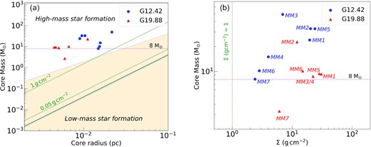
(a) The mass of the compact cores, identified using the 3 mm and 2.7 mm maps of G12.42+0.50, and G19.88−0.53, respectively, is plotted as a function of the radius of the cores, and depicted by circles. The cyan and black lines indicate the surface density thresholds of 116 |$\rm M_\odot$|pc−2 (∼ 0.024 g cm−2) and 129 |$\rm M_\odot$|pc−2 (∼ 0.027 g cm−2) for active star formation from Lada, Lombardi & Alves (2010) and Heiderman et al. (2010), respectively. The shaded region delineates the low-mass star-forming region that does not satisfy the criterion m(r) > 870 |$\rm M_\odot (r$|/pc)1.33 (Kauffmann et al. 2010).The green dashed lines represent the surface density threshold of 0.05 and 1 g cm−2 defined by Krumholz & McKee (2008) and Urquhart et al. (2014), respectively. (b) Core mass as a function of core mass surface density is shown. The green vertical line indicates a theoretical threshold of 1 g cm−2, above which the cores most likely form high-mass stars. The horizontal magenta line in both plots indicates a core mass of 8 |$\rm M_\odot$|.
We rule out the effect of mass sensitivity (refer Section 3) on the observed lack of low-mass cores. Dearth of low-mass cores in star-forming clumps has also been reported by several authors (e.g. Zhang et al. 2015; Liu et al. 2017). Later formation epoch of low-mass stars and feedback from newly formed massive stars suppressing further fragmentation are some of the likely reasons discussed in these papers. In this study, collimated and large-scale outflows are identified towards G12.42 and G19.88 (Section 6.3). Further, Issac19 suggest a co-existence of the UC H ii region with an ionized jet in the G12.42 complex. Hence, the presence of multiple outflows and an UC H ii region would have possibly inhibited further fragmentation resulting in the observed lack of low-mass protostellar cores.
6 GAS KINEMATICS IN THE MULTISCALE STRUCTURES ASSOCIATED WITH THE PROTOCLUSTERS
6.1 Large-scale filamentary structures
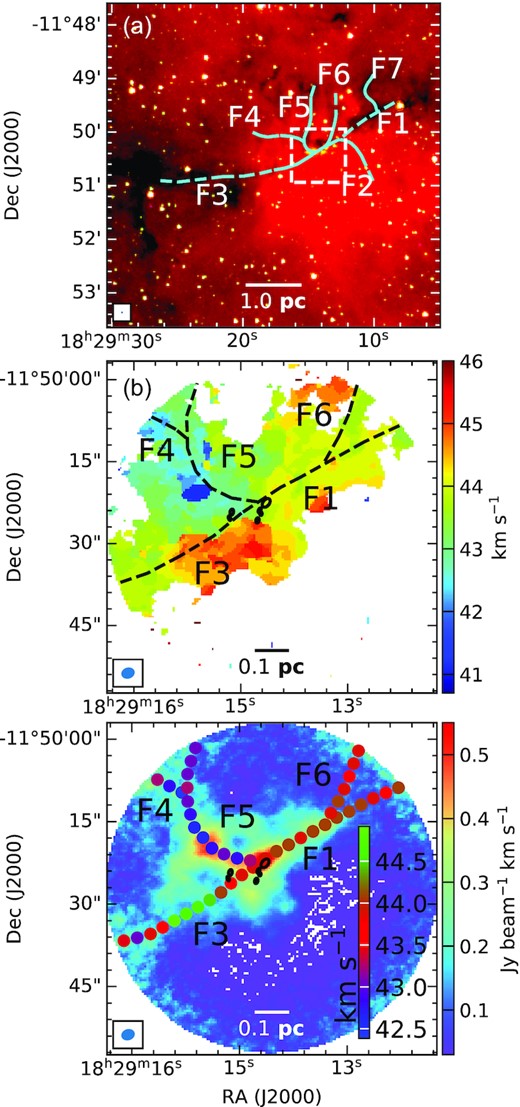
G12.42 has been proposed as a hub-filament system by Issac19 based on the morphology seen in mid-infrared Spitzer and far-infrared Herschel images. Using the 8 |$\rm \mu m$| Spitzer image, where the filamentary structures appear as dark (high extinction) lanes, these authors have visually identified six large-scale filamentary structures (F1 – F6) in the south-west merging towards the central clump. When overlaid on the 350 |$\rm \mu m$| Herschel image, these identified filaments match with the bright, filamentary far-infrared emission (refer fig. 7 of Issac19). Further, using |$\rm ^{12}CO (3-2)$| molecular line data from JCMT, they also reveal bulk motion along the identified filaments and conjecture this as gas inflow. Following similar approach, we revisited the filament identification in G12.42 and detected three additional filaments (F7–F9). In Fig. 10, we present the morphology and gas kinematics in this hub-filament system. From Fig. 10(a), two hubs with intertwining filaments can be discerned where the protocluster, G12.42, is associated with the north-east hub. The large-scale network of filaments is also seen in the JCMT |$\rm {}^{13}$|CO(3–2) velocity integrated map (Fig. 10b). For better signal-to-noise ratio, the map is convolved to a resolution of 35 arcsec.
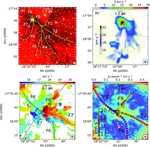
(a) Skeletons of the identified filaments are overlaid on the colour composite image of the region around G12.42 using Spitzer 3.6 |$\mu$|m (blue), 4.5 |$\mu$|m (green), and 8.0 |$\mu$|m (red) bands. The yellow dashed curves are adopted from Issac19 and the cyan dashed curves are new filaments identified in this paper. (b) Moment zero map of |$\rm ^{13}$|CO (3–2) molecular line data from JCMT is shown in colour scale. The velocity peaks of |$\rm ^{12}$|CO (3–2) adopted from Issac19 are overlaid on it. The dashed square box represents the region of the ATOMS maps shown in panels (c) and (d). (c) Peak velocity map of |$\rm H^{13}CO^{+}$| (1–0) (obtained using combined 12-m + 7-m data) overlaid with filaments F2, F6, F7, F8, and F9. (d) The velocity peaks of |$\rm H^{13}CO^{+}$| (1–0) extracted along the filaments (F2, F6, F8, and F9) are overlaid on the moment zero map of |$\rm H^{13}CO^{+}$| (1–0) for the region associated with G12.42+0.50 shown in colour scale. The identified 3 mm cores are shown as black ellipses. The beam sizes are shown at the bottom right of each figure.
The velocity structure (illustrated as colour coded circles) along the identified MIR filaments by Issac19 are overplotted on the |$\rm {}^{13}$|CO(3–2) velocity integrated map. The circles depict the |$\rm {}^{12}$|CO(3–2) peak velocities obtained within circular regions of radius 3.75 arcsec. Filamentary structures seen in the molecular line map display more extended and complex morphologies. To avoid optical depth effects and influence of outflows, it would have been ideal to obtain the velocity structure using the optically thin |$\rm {}^{13}$|CO(3–2) transition but such an analysis was not possible due to poor signal-to-noise ratio where the peak fluxes within the apertures along the filaments are less than three times the rms noise. As illustrated by the colour coded circles, clear velocity gradients |$\sim 1\, \rm km\, s^{-1}{pc}^{-1}$| are seen along the identified filaments with decreasing velocities as one moves towards the hubs.
The ATOMS survey has probed the inner region of the central hub in G12.42. We investigate the gas kinematics in this region by constructing the peak velocity map using the high resolution (∼2.5 arcsec) H13CO+(1-0) ALMA data. In doing so we have considered only the pixels where the peak intensity along the spectral axis is greater than five times rms. The map is shown in Fig. 10(c) where the identified filaments are drawn. To further elaborate on the velocity structure, we estimate the median values of the peak velocities within circles of radius 1.25 arcsec along the filaments. These are shown in Fig. 10(d) as colour-coded circles overlaid on the moment zero map of H13CO+. The velocity structure for F7 is not plotted since the peak velocities are masked out (pixel values below five times rms) along most part of the filament. Along the filaments F2, F8, and F9, the overall velocity gradient is ∼ 2|$\, \rm km\, s^{-1}{pc}^{-1}$|. Considering the filament F6, the velocity field is comparatively complex and shows variation. In the inner region, however, the gradient along the filaments F2, F6, and F9 become steeper. The velocity structure also reveals reversals, jump discontinuities which are difficult to interpret given the complex kinematics associated with the active star-forming cores.
Study of other star-forming regions, like the SDC335 cluster (Peretto et al. 2013), Serpens South cluster (Kirk et al. 2013), and AFL5142 (Liu et al. 2016) has revealed evidence of velocity gradients along filaments. Peretto et al. (2013) and Kirk et al. (2013) interpreted velocity gradients of the order of |$\sim 1\, \rm km\, s^{-1}{pc}^{-1}$| as gas infiow along filaments. Further, the median values of the velocities along filaments F2 and F9 are |$\sim 19\, \rm km\, s^{-1}$| and that along F6 and F8 are |$\sim 17.5\, \rm km\, s^{-1}$|, spanning two different ranges. This is consistent with double-peaked profiles seen in the grid presented in Section 4.
The presence of such large-scale filaments is also seen in G19.88 as illustrated in Fig. 11(a), where, following the same approach as in G12.42, we have visually identified seven filaments (F1–F7) that are seen intersecting at the central hub harbouring the protocluster. Proceeding along the lines discussed for G12.42, the overlay of these filaments on the ATOMS H13CO+(1–0) peak velocity map is shown in Fig. 11(b) and the colour-coded velocity structure is shown on the H13CO+(1–0) moment zero map. The overall velocity gradients along the identified filaments are much lower (|$\lt 0.5\, \rm km\, s^{-1}{pc}^{-1}$|) compared to the filaments in G12.42. However, steep velocity fluctuations are seen in F3 and F5. Gas kinematics of the large-scale filaments in this protocluster could not be explored due to unavailability of good quality archival CO molecular line data. It is worth mentioning here that using data from ATOMS survey, Zhou et al. (2022) has identified well-defined network of filaments in both these protoclusters by applying the FILFINDER algorithm on the moment zero maps of H13CO+(1–0). These identified filaments appear to match well with the visually identified MIR filaments presented in this work. Further, the multiple outflows detected in both protoclusters (discussed in a later section) influence the kinematics of the inflowing gas along the filaments.
(a) Skeletons of the identified filaments are overlaid on the colour composite image of the region around G19.88 using Spitzer 3.6 |$\mu$|m (blue), 4.5 |$\mu$|m (green), and 8.0 |$\mu$|m (red) bands. The dashed square box represents the region of the ATOMS maps shown in panels (b) and (c). (b) Peak velocity map of |$\rm H^{13}CO^{+}$| (1–0) (obtained using combined 12-m + 7-m data) overlaid with filaments F1, F3, F4, F5, and F6 is shown in colour scale. (c) The velocity peaks of |$\rm H^{13}CO^{+}$| (1–0) extracted along the filaments (F1, F3, F4, F5, and F6) are overlaid on the moment zero map of |$\rm H^{13}CO^{+}$| (1–0) for the region associated with G19.88−0.53 shown in colour scale. Ellipses represent the identified 2.7 mm cores. The beam sizes are shown at the bottom left of each figure.
6.2 Small-scale density structures
To delve deeper and understand the dynamics that drives the star formation process in the two protoclusters, we perform a dendrogram analysis along the lines discussed in Liu et al. (2022b) for the filamentary cloud G034.43+00.24. Density structures at two different scales (branches and leaves) are identified using the H13CO+ data cube in position–position–velocity (PPV) space. As mentioned in Section 3.1 the dendrogram technique decomposes the emission into a hierarchy of substructures where leaves are the smallest, bright structures at the top of the tree hierarchy and branches are the faint, extended structures lower down in the tree. The local maxima in the data set determine the dendrogram structures defined by distinct isosurfaces around and containing these local maxima. Presence of noisy pixels introduces spurious local maxima. To minimize this, we first generate a noise map where each pixel represents the standard deviation of intensity of that pixel in the line-free channels of the data cube spanning 30 km s−1. Using this noise map, a modified data cube of H13CO+ is made, where pixels having peak intensity (along the spectral axis) less than five times the noise are masked out.
To generate the dendrogram tree, the following parameters are used: (i) |$min\_value = 5 \sigma$|, (ii) |$min\_delta = 2 \sigma$|, and (iii) |$min\_npix = N$| pixels. N is taken to be five times the synthesized beam area to increase the possibility that the detected structures are resolved both spatially (at least 3 beams) and in velocity (at least 2 channels). Further details regarding the selection of dendrogram parameters can be found in Duarte-Cabral et al. (2021). The values of σ and N for G12.42 and G19.88 are 0.007, 0.008 |$\rm Jy\, beam^{-1}$|, and 175, 177, respectively. Figs 12(a) and (b) display the 2D spatial distribution of the detected leaves overlaid on the moment zero map of the modified data cube of H13CO+ for G12.42 and G19.88, respectively. Based on a careful visual scrutiny, we discarded structures 15, 36, and 41 associated with G12.42 for further analysis. These structures are located at the edge and appear truncated. Following the above procedure, we obtain 23 leaves and 15 branches for G12.42 and for G19.88, 11 leaves and 5 branches are identified.
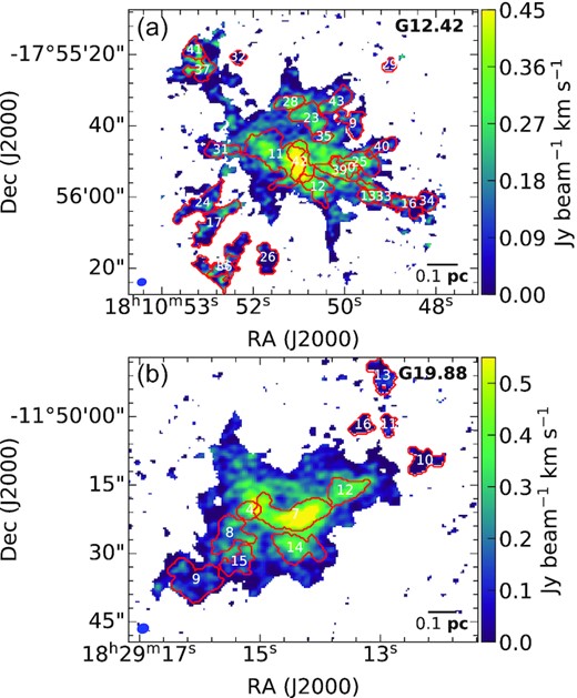
(a) Moment zero map of the modified |$\rm H^{13}CO^{+}$| cube where only the pixels having peak intensity (along the spectral axis) greater than five times the noise are shown. The overlaid apertures are 2D representations of the 3D (PPV) leaf structures identified in G12.42. Each leaf is labelled with its structure ID (refer Table 7). (b) Same as (a) but for G19.88. The beam sizes are shown at the bottom left of each figure.
The basic parameters of the identified density structures are tabulated in Tables 7 and 8. These include the coordinates, corrected major and minor axes, the aspect ratio, size, the peak intensity, the velocity range in which the structures span, the mean velocity, <Vlsr>, of the structures, the velocity variation, δV, and the mean velocity dispersion, <σ> of each identified structures. As discussed and implemented in Liu et al. (2022b), a correction factor is multiplied to the major and minor axes. This factor equals the square root of the ratio of the actual area of the density structure in the plane of the sky to the area of the dendrogram extracted ellipse. The intensity-weighted first moment map is used to estimate the mean velocity (<Vlsr>) over the associated velocity range of the structure. The velocity variation δV is the standard deviation of Vlsr in the structures and the mean velocity dispersion (<σ>) is determined from the intensity-weighted second moment map. Using equation (9), the non-thermal velocity dispersion (|$\rm \sigma _{\rm nt}$|) is calculated, where σline is replaced by the mean velocity dispersion (<σ>) values given in Tables 7 and 8. The clump averaged Tkin from Wienen et al. (2012) (refer Section 5) is considered in the calculation of σnt.
Physical parameters of leaves for G12.42 and G19.88.
| ID | RA | DEC | major | minor | Aspect | Length | FP | Vel. range | <Vlsr> | δV | <σ> | <σnt> |
|---|---|---|---|---|---|---|---|---|---|---|---|---|
| (J2000) | (J2000) | (arcsec) | (arcsec) | ratio | pc | |$\rm Jy\, beam^{-1}$| | km s−1 | km s−1 | km s−1 | km s−1 | km s−1 | |
| G12.42 | ||||||||||||
| 0 | 18:10:49.67 | −17:55:51.84 | 2.1 | 1.4 | 0.69 | 0.02 | 0.05 | [13.51, 14.77] | 14.08 ± 0.06 | 0.20 ± 0.04 | 0.40 ± 0.03 | 0.40 ± 0.03 |
| 9 | 18:10:49.64 | −17:55:39.44 | 3.3 | 2.1 | 0.65 | 0.03 | 0.07 | [15.61, 17.51] | 16.44 ± 0.05 | 0.45 ± 0.04 | 0.48 ± 0.02 | 0.47 ± 0.02 |
| 11 | 18:10:51.15 | −17:55:48.07 | 8.3 | 3.8 | 0.46 | 0.07 | 0.30 | [15.83, 18.15] | 16.98 ± 0.01 | 0.26 ± 0.01 | 0.60 ± 0.01 | 0.59 ± 0.01 |
| 12 | 18:10:50.33 | −17:55:57.25 | 3.8 | 2.3 | 0.62 | 0.03 | 0.18 | [16.04, 17.72] | 16.88 ± 0.04 | 0.34 ± 0.03 | 0.50 ± 0.01 | 0.50 ± 0.01 |
| 13 | 18:10:49.34 | −17:55:59.87 | 2.5 | 1.6 | 0.63 | 0.02 | 0.15 | [16.25, 16.88] | 16.58 ± 0.05 | 0.07 ± 0.04 | 0.21 ± 0.04 | 0.20 ± 0.04 |
| 16 | 18:10:48.54 | −17:56:02.02 | 3.8 | 1.9 | 0.5 | 0.03 | 0.10 | [16.46, 17.72] | 17.10 ± 0.04 | 0.25 ± 0.03 | 0.27 ± 0.02 | 0.26 ± 0.02 |
| 17 | 18:10:52.37 | −17:56:07.36 | 7.0 | 2.0 | 0.28 | 0.04 | 0.16 | [16.46, 18.15] | 17.20 ± 0.02 | 0.17 ± 0.02 | 0.43 ± 0.01 | 0.43 ± 0.01 |
| 23 | 18:10:50.46 | −17:55:37.98 | 4.4 | 2.6 | 0.6 | 0.04 | 0.20 | [16.67, 19.20] | 17.94 ± 0.04 | 0.59 ± 0.03 | 0.74 ± 0.01 | 0.74 ± 0.01 |
| 24 | 18:10:52.59 | −17:56:01.70 | 6.5 | 1.9 | 0.29 | 0.04 | 0.15 | [16.88, 18.36] | 17.64 ± 0.02 | 0.20 ± 0.02 | 0.43 ± 0.01 | 0.43 ± 0.01 |
| 25 | 18:10:49.51 | −17:55:50.32 | 5.8 | 2.1 | 0.36 | 0.04 | 0.17 | [16.88, 18.57] | 17.74 ± 0.03 | 0.29 ± 0.02 | 0.50 ± 0.01 | 0.50 ± 0.01 |
| 26 | 18:10:51.31 | −17:56:17.06 | 3.6 | 2.2 | 0.59 | 0.03 | 0.13 | [17.30, 18.57] | 17.99 ± 0.04 | 0.13 ± 0.03 | 0.14 ± 0.02 | 0.12 ± 0.02 |
| 28 | 18:10:50.87 | −17:55:33.44 | 3.6 | 1.5 | 0.41 | 0.03 | 0.20 | [17.51, 18.15] | 17.86 ± 0.05 | 0.09 ± 0.04 | 0.22 ± 0.03 | 0.21 ± 0.03 |
| 29 | 18:10:48.92 | −17:55:22.94 | 1.5 | 1.3 | 0.86 | 0.02 | 0.10 | [17.51, 18.99] | 18.23 ± 0.07 | 0.11 ± 0.05 | 0.37 ± 0.05 | 0.37 ± 0.05 |
| 31 | 18:10:52.24 | −17:55:46.81 | 4.4 | 1.3 | 0.29 | 0.03 | 0.16 | [18.15, 18.99] | 18.54 ± 0.05 | 0.18 ± 0.03 | 0.28 ± 0.02 | 0.27 ± 0.02 |
| 32 | 18:10:51.89 | −17:55:20.80 | 1.6 | 1.5 | 0.94 | 0.02 | 0.11 | [18.15, 18.99] | 18.61 ± 0.08 | 0.11 ± 0.06 | 0.23 ± 0.05 | 0.22 ± 0.05 |
| 33 | 18:10:49.03 | −17:55:59.99 | 5.7 | 1.5 | 0.26 | 0.03 | 0.22 | [18.36, 19.20] | 18.85 ± 0.03 | 0.20 ± 0.02 | 0.27 ± 0.02 | 0.26 ± 0.02 |
| 34 | 18:10:48.18 | −17:56:01.22 | 2.4 | 2.1 | 0.85 | 0.03 | 0.19 | [18.36, 18.78] | 18.58 ± 0.05 | 0.06 ± 0.04 | 0.16 ± 0.04 | 0.14 ± 0.04 |
| 35 | 18:10:50.21 | −17:55:43.11 | 2.2 | 1.2 | 0.54 | 0.02 | 0.15 | [18.36, 19.20] | 18.76 ± 0.07 | 0.15 ± 0.05 | 0.29 ± 0.04 | 0.29 ± 0.04 |
| 37 | 18:10:52.60 | −17:55:24.46 | 3.2 | 1.8 | 0.54 | 0.03 | 0.21 | [18.57, 19.41] | 18.98 ± 0.04 | 0.24 ± 0.03 | 0.28 ± 0.02 | 0.27 ± 0.02 |
| 39 | 18:10:49.90 | −17:55:52.62 | 5.1 | 1.7 | 0.33 | 0.03 | 0.19 | [18.78, 19.62] | 19.18 ± 0.03 | 0.13 ± 0.02 | 0.27 ± 0.02 | 0.27 ± 0.02 |
| 40 | 18:10:49.07 | −17:55:46.02 | 4.2 | 1.0 | 0.25 | 0.02 | 0.11 | [18.78, 19.62] | 19.18 ± 0.04 | 0.14 ± 0.03 | 0.28 ± 0.03 | 0.27 ± 0.03 |
| 42 | 18:10:50.69 | −17:55:50.18 | 5.4 | 2.3 | 0.42 | 0.04 | 0.26 | [18.99, 20.68] | 19.84 ± 0.03 | 0.33 ± 0.02 | 0.46 ± 0.01 | 0.46 ± 0.01 |
| 43 | 18:10:49.96 | −17:55:33.27 | 4.8 | 1.7 | 0.35 | 0.03 | 0.17 | [18.99, 19.83] | 19.37 ± 0.03 | 0.12 ± 0.02 | 0.27 ± 0.02 | 0.26 ± 0.02 |
| G19.88 | ||||||||||||
| 4 | 18:29:15.15 | −11:50:20.56 | 2.2 | 1.4 | 0.65 | 0.03 | 0.20 | [40.70, 41.75] | 41.22 ± 0.05 | 0.08 ± 0.04 | 0.34 ± 0.04 | 0.33 ± 0.04 |
| 7 | 18:29:14.47 | −11:50:21.46 | 6.7 | 2.5 | 0.37 | 0.07 | 0.33 | [42.17, 44.71] | 43.47 ± 0.03 | 0.53 ± 0.02 | 0.70 ± 0.01 | 0.70 ± 0.01 |
| 8 | 18:29:15.45 | −11:50:25.58 | 3.4 | 2.6 | 0.74 | 0.05 | 0.16 | [42.60, 44.07] | 43.32 ± 0.03 | 0.23 ± 0.02 | 0.45 ± 0.01 | 0.44 ± 0.01 |
| 9 | 18:29:15.95 | −11:50:35.79 | 4.8 | 3.2 | 0.67 | 0.06 | 0.14 | [43.23, 44.28] | 43.78 ± 0.02 | 0.13 ± 0.02 | 0.32 ± 0.01 | 0.31 ± 0.01 |
| 10 | 18:29:12.54 | −11:50:09.69 | 2.9 | 2.0 | 0.69 | 0.04 | 0.12 | [43.23, 44.49] | 43.68 ± 0.06 | 0.28 ± 0.05 | 0.31 ± 0.03 | 0.31 ± 0.03 |
| 11 | 18:29:13.07 | −11:50:01.76 | 2.0 | 1.0 | 0.52 | 0.02 | 0.08 | [43.23, 44.28] | 43.78 ± 0.08 | 0.14 ± 0.06 | 0.31 ± 0.05 | 0.30 ± 0.05 |
| 12 | 18:29:13.73 | −11:50:16.25 | 3.6 | 2.0 | 0.55 | 0.04 | 0.26 | [43.44, 44.49] | 44.00 ± 0.04 | 0.16 ± 0.03 | 0.33 ± 0.02 | 0.32 ± 0.02 |
| 13 | 18:29:13.17 | −11:49:51.05 | 3.2 | 1.9 | 0.58 | 0.04 | 0.13 | [43.65, 44.71] | 44.06 ± 0.05 | 0.11 ± 0.03 | 0.25 ± 0.03 | 0.24 ± 0.03 |
| 14 | 18:29:14.48 | −11:50:28.82 | 4.3 | 2.5 | 0.57 | 0.05 | 0.20 | [43.86, 45.76] | 44.76 ± 0.03 | 0.32 ± 0.02 | 0.54 ± 0.01 | 0.54 ± 0.01 |
| 15 | 18:29:15.31 | −11:50:31.83 | 3.2 | 1.7 | 0.52 | 0.04 | 0.11 | [44.28, 44.92] | 44.59 ± 0.05 | 0.16 ± 0.03 | 0.23 ± 0.03 | 0.22 ± 0.03 |
| 16 | 18:29:13.46 | −11:50:01.83 | 2.1 | 1.5 | 0.71 | 0.03 | 0.10 | [44.28, 45.13] | 44.73 ± 0.06 | 0.06 ± 0.05 | 0.27 ± 0.04 | 0.26 ± 0.04 |
Physical parameters of branches for G12.42 and G19.88.
| ID | RA | DEC | major | minor | Aspect | Length | FP | Vel. range | <Vlsr> | δV | <σ> | <σnt> |
|---|---|---|---|---|---|---|---|---|---|---|---|---|
| (J2000) | (J2000) | (arcsec) | (arcsec) | ratio | pc | |$\rm Jy\, beam^{-1}$| | km s−1 | km s−1 | km s−1 | km s−1 | km s−1 | |
| G12.42 | ||||||||||||
| 2 | 18:10:50.66 | −17:55:45.87 | 27.92 | 13.64 | 0.49 | 0.23 | 0.30 | [14.77, 21.10] | 18.02 ± 0.01 | 1.14 ± 0.01 | 1.16 ± 0.006 | 1.15 ± 0.006 |
| 3 | 18:10:50.67 | −17:55:45.87 | 27.88 | 13.40 | 0.48 | 0.22 | 0.30 | [14.98, 21.10] | 18.02 ± 0.01 | 1.02 ± 0.01 | 1.16 ± 0.005 | 1.15 ± 0.005 |
| 4 | 18:10:50.45 | −17:55:48.43 | 21.58 | 13.68 | 0.63 | 0.20 | 0.30 | [14.98, 21.10] | 17.94 ± 0.01 | 0.91 ± 0.01 | 1.16 ± 0.005 | 1.15 ± 0.005 |
| 5 | 18:10:50.44 | −17:55:48.37 | 19.42 | 11.66 | 0.60 | 0.18 | 0.30 | [15.19, 20.89] | 17.95 ± 0.01 | 1.10 ± 0.01 | 1.16 ± 0.002 | 1.16 ± 0.002 |
| 6 | 18:10:50.45 | −17:55:48.28 | 19.24 | 11.66 | 0.61 | 0.17 | 0.30 | [15.19, 20.89] | 17.95 ± 0.01 | 1.06 ± 0.01 | 1.16 ± 0.006 | 1.16 ± 0.006 |
| 7 | 18:10:51.01 | −17:55:50.71 | 15.11 | 6.20 | 0.41 | 0.11 | 0.30 | [15.19, 19.20] | 17.43 ± 0.01 | 0.70 ± 0.01 | 0.95 ± 0.003 | 0.95 ± 0.003 |
| 8 | 18:10:50.95 | −17:55:50.47 | 13.91 | 4.58 | 0.33 | 0.09 | 0.30 | [15.40, 18.36] | 17.09 ± 0.01 | 0.48 ± 0.01 | 0.71 ± 0.004 | 0.70 ± 0.004 |
| 14 | 18:10:52.56 | −17:55:23.53 | 9.55 | 5.81 | 0.61 | 0.09 | 0.21 | [16.25, 20.04] | 19.07 ± 0.02 | 0.73 ± 0.02 | 0.48 ± 0.005 | 0.47 ± 0.005 |
| 18 | 18:10:50.08 | −17:55:46.79 | 17.42 | 7.76 | 0.45 | 0.14 | 0.26 | [16.46, 20.89] | 18.28 ± 0.01 | 0.86 ± 0.01 | 1.07 ± 0.004 | 1.07 ± 0.004 |
| 19 | 18:10:50.14 | −17:55:47.30 | 16.63 | 6.63 | 0.4 | 0.12 | 0.26 | [16.46, 20.89] | 18.28 ± 0.01 | 0.85 ± 0.01 | 1.08 ± 0.003 | 1.07 ± 0.003 |
| 20 | 18:10:50.09 | −17:55:47.49 | 17.21 | 6.93 | 0.4 | 0.13 | 0.26 | [16.46, 20.89] | 18.28 ± 0.01 | 0.91 ± 0.01 | 1.08 ± 0.004 | 1.07 ± 0.004 |
| 21 | 18:10:50.18 | −17:55:47.66 | 14.16 | 5.87 | 0.41 | 0.11 | 0.26 | [16.67, 20.68] | 18.35 ± 0.02 | 0.88 ± 0.01 | 1.05 ± 0.003 | 1.05 ± 0.003 |
| 22 | 18:10:50.52 | −17:55:37.62 | 7.96 | 2.81 | 0.35 | 0.06 | 0.20 | [16.67, 19.20] | 17.98 ± 0.03 | 0.66 ± 0.02 | 0.72 ± 0.007 | 0.72 ± 0.007 |
| 30 | 18:10:50.03 | −17:55:52.74 | 14.12 | 3.62 | 0.26 | 0.08 | 0.26 | [18.15, 20.68] | 19.18 ± 0.01 | 0.49 ± 0.01 | 0.63 ± 0.005 | 0.62 ± 0.005 |
| 38 | 18:10:50.40 | −17:55:50.64 | 7.20 | 3.39 | 0.47 | 0.06 | 0.26 | [18.78, 20.68] | 19.54 ± 0.02 | 0.40 ± 0.02 | 0.51 ± 0.005 | 0.51 ± 0.005 |
| G19.88 | ||||||||||||
| 1 | 18:29:14.57 | −11:50:20.96 | 13.87 | 8.13 | 0.59 | 0.17 | 0.33 | [40.70, 45.76] | 43.51 ± 0.01 | 0.82 ± 0.01 | 1.09 ± 0.004 | 1.08 ± 0.004 |
| 2 | 18:29:14.61 | −11:50:21.16 | 14.89 | 8.97 | 0.6 | 0.19 | 0.33 | [40.70, 45.76] | 43.56 ± 0.01 | 0.92 ± 0.01 | 1.08 ± 0.004 | 1.08 ± 0.004 |
| 3 | 18:29:14.42 | −11:50:20.77 | 11.04 | 6.44 | 0.58 | 0.14 | 0.33 | [40.70, 45.76] | 43.54 ± 0.02 | 0.95 ± 0.01 | 1.14 ± 0.004 | 1.13 ± 0.004 |
| 5 | 18:29:14.37 | −11:50:19.65 | 11.94 | 4.22 | 0.35 | 0.11 | 0.33 | [40.70, 45.13] | 43.28 ± 0.02 | 0.90 ± 0.02 | 1.06 ± 0.005 | 1.05 ± 0.005 |
| 6 | 18:29:14.34 | −11:50:19.64 | 11.44 | 4.19 | 0.37 | 0.11 | 0.33 | [41.96, 45.13] | 43.55 ± 0.02 | 0.57 ± 0.01 | 0.81 ± 0.006 | 0.81 ± 0.006 |
Consistent with the dendrogram tree hierarchy, on average the leaves display larger aspect ratios compared to the branches and have sizes that are smaller by a factor of ∼4. The average velocities of the structures reflect the dominant velocity components associated with the protoclusters. It should, however, be noted here that the double velocity component observed in G12.42 will be ingrained in the kinematics of the structures. Compared to the structures identified in G034.43+00.2 (Liu et al. 2022b) where the leaves and branches were typically 0.09 and 0.6 pc, respectively, we are probing smaller scale density structures in G12.42 and G19.88 where the median values of leaves and branches are 0.03 and 0.1 pc, respectively. To decipher the gas dynamics of these two protoclusters, we investigate the derived values of |$\rm \delta V$| and |$\rm \sigma _{nt}$| of small and larger-scale density structures detected. The parameter δV represents the gas kinematics within the density structure in the plane of the sky and σnt gives the mean gas motion along the line of sight (Lee et al. 2014; Storm et al. 2014; Liu et al. 2022b). In Fig. 13, we plot both these parameters as a function of the size-scale, L. The branches have larger δV and σnt than the leaves, which is consistent with the fact that these cover larger spatial scales and hence likely to reflect large-scale gas motion. Similar velocity trends are seen in the analysis of the density structures in G034.43+00.24 (Liu et al. 2022b). The velocity regimes are indicated in the figure. The shaded horizontal band delimitates the sonic (≤ceff) and the transonic (≤2ceff) levels at 0.3 and 0.6 |$\rm km\, s^{-1}$|, respectively. The clump-averaged Tkin is used in equation (7) to calculate the above levels. The velocity variation, δV, of majority of the leaves is below the sonic level while most of the branches are above the transonic regime. The distribution in the mean non-thermal velocity dispersion also shows similar behaviour. This shows that gas motions in the larger scale density structures, the branches, are mostly supersonic while in the smaller scale structures, the leaves, subsonic, or transonic gas motion is observed.
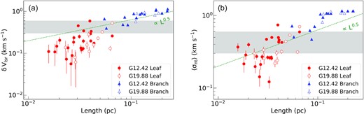
Velocity size relation for density structures in G12.42 and G19.88. (a) Variation of velocity plotted as a function of size. (b) Non-thermal velocity dispersion as a function of size. In both the panels, circles indicate the leaf structures and triangles show dendrogram branches. The filled and empty markers represent values for G12.42 and G19.88, respectively. In both the panels, the green dashed line shows the Larson relation with C = 2.0 and Γ = 0.5.
Internal kinematics of molecular clouds are known to be dominated by supersonic gas motion that is generally attributed to turbulent gas flow, chaotic gravity-driven motions, or orderly large-scale gas inflow (Hacar et al. 2016; Liu et al. 2022b, and references therein). For turbulent clouds, there exists a correlation between the velocity field and the size which takes a power-law form over a large range of spatial scales probed. This is referred to as Larson’s law (velocity dispersion, |$\sigma (\rm km\, s^{-1}$|) |$\simeq C~ L(\rm pc)^{\Gamma }$|, with coefficients C = 1.1 and Γ = 0.38) after the pioneering work by Larson (1981). Following this, several observational and simulation studies (e.g. Larson 1981; Solomon et al. 1987; Heyer & Brunt 2004; Rosolowsky et al. 2008) have shown this power-law scaling in molecular clouds to be consistent with the presence of turbulence, supersonic motions, and shocks due to colliding gas flows. These studies have revealed that the scaling exponent and coefficient show near invariance suggesting the universality of turbulence. Based on several later studies on larger and more homogeneous data sets, the widely accepted values are C = 1.0 and Γ = 0.5 (Solomon et al. 1987).
To probe this scaling at the scales of the structures in G12.42 and G19.88, the Larson relation with a power-law exponent of 0.5 is shown in Fig. 13. The Larson coefficient (1.0; Solomon et al. 1987) has been offset to the level of the observed velocity parameters. The branches show trends in both plots that are consistent with the canonical Larson’s relation slope. The scatter seen in the leaves is larger but there is a definite hint of deviation (i.e. steepening) which is visually more prominent in the L − δV plot. Similar studies have been carried out by several authors and in the discussion that follows we give a brief overview of the same. The velocity–size scaling in G034.43+00.24 (Liu et al. 2022b) also shows similar steepening for the leaf structures. Other recent studies based on high-resolution data (e.g. Ballesteros-Paredes et al. 2011; Friesen et al. 2016; Hacar et al. 2016) have also shown deviation from the Larson law both in the scaling exponent and coefficient. Dendrogram analysis of the linewidth–size relation in Serpens South, using |$\rm NH_3$| molecular line data, shows a flat L − σnt distribution (Friesen et al. 2016). For Serpens Mains, Lee et al. (2014) implemented similar analysis with |$\rm N_2H^+$|(1–0) data and present consistent results where σnt remains invariant with size though the L − δV slope agrees well with the Larson relation. In their analysis of the sonic filament in the Musca cloud, Hacar et al. (2016) report a broken power-law fit where a flattening is seen shortward of ∼1 pc.
Summarizing the results of these above-mentioned studies and comparing the same with our work, it is possible that local gas kinematics in regions within molecular clouds is different while still preserving the global properties described by the Larson relation. Additionally, the observed deviations reflect the spatial scales at which turbulence ceases to dominate the kinematics of the cloud. The velocity structure seen in the Musca filament (Hacar et al. 2016) is the first observational evidence of a parsec-scale structure that is fully decoupled from the supersonic turbulent regime of the ISM. Another crucial piece of information that is gathered from the L − δV and the L − σnt plots for G12.42 and G19.88 is the transition from supersonic gas motion to transonic velocities at ∼0.1 pc. This is in excellent agreement with the observational results presented in Goodman et al. (1998) and Pineda et al. (2010) and defines the transitional scale at which turbulent gas motion dissipates. From the observed |$\rm NH_3$| line width variation, Wang et al. (2008) have also inferred dissipation of turbulence occurring in the dense regions of the infrared dark cloud G28.34−0.06. At this juncture, the turbulence induced non-linear density fluctuations proceed towards formation of sonic substructures which eventually form the star-forming cores. Hence, for the identified structures within our protoclusters, the deviation from Larson’s scaling and the transition scale from supersonic motion corroborate well with each other.
6.3 Core kinematics
6.3.1 Infall activity
Following the analysis presented in Section 4, the virial mass and virial parameter are calculated for all the detected cores and tabulated in Table 9. αvir values are estimated to be less than 2 for all cores. As conjectured for the clumps, the detected cores can also be considered to be supercritical and under collapse. And if that is not the case, then there should exist significant support (e.g. magnetic field) to resist collapse (see Section 4).
Virial parameters of cores associated with G12.42+0.50 and G19.88−0.53.
| Cores | Line width (ΔV) | Mvir | αvir |
|---|---|---|---|
| |$\rm km\, s^{-1}$| | (|$\rm M_{\odot }$|) | ||
| G12.42 | |||
| MM1 | 1.2 | 2.0 | 0.1 |
| MM2 | 1.2 | 2.1 | 0.1 |
| MM3 | 1.4 | 6.3 | 0.1 |
| MM4 | 1.7 | 6.3 | 0.4 |
| MM5 | 1.6 | 3.5 | 0.1 |
| MM6 | 1.0 | 2.2 | 0.2 |
| MM7 | 0.9 | 1.9 | 0.2 |
| G19.88 | |||
| MM1 | 2.1 | 2.9 | 0.3 |
| MM2 | 1.6 | 4.1 | 0.2 |
| MM3 | 2.1 | 3.1 | 0.4 |
| MM4 | 2.1 | 3.1 | 0.4 |
| MM5 | 2.0 | 2.9 | 0.3 |
| MM6 | 2.0 | 4.2 | 0.4 |
| MM7 | 2.1 | 3.7 | 1.1 |
In addition to the above, from the spectra presented in Figs 6 and 7, several cores are seen to display the typical infall signature. For G12.42, the cores, MM1, MM2, and MM3 clearly show self-absorbed profiles of |$\rm HCO^+$|. In case of G19.88, the spectrum extracted over the area covering the cores MM1, MM3, MM4, and MM7 shows this signature. It is difficult in this case to attribute this to any particular core. Using equation (4), we also estimate the asymmetry parameter (A) for these core profiles which lie in the range −0.6 to −0.7. These estimated values in combination with the displayed profiles of the |$\rm HCO^+$| and the H13CO+ lines strongly indicate infall activity in these cores. Furthermore, assuming a spherically symmetric core of radius, Rcore, and volume density, ρ, we estimate the mass infall rate, Minf = |$4\pi R^{2}_{\rm core}\rho V_{\rm inf}$| (López-Sepulcre, Cesaroni & Walmsley 2010), where |$V_{\rm inf} = |V_{\rm thick} - V_{\rm thin}| = |V_{\rm H^{13}CO^{+}} - V_{\rm HCO^{+}}|$| is the infall velocity and |$\rho = M_{\rm core} \big / \frac{4}{3}\pi R^{3}_{\rm core}$|. For the individual cores probed in G12.42, |$M\rm _{inf}$| is estimated to be |$\sim 6.5\times 10^{-3}\, \rm M_{\odot } yr^{-1}$|. For G19.88, the spectra showing infall yield similar values ranging from ∼1.4 × 10⁻³ to |$\sim 6.3\times 10^{-3}\, \rm M_{\odot } yr^{-1}$|. These are in good agreement with infall rates derived for other high-mass star-forming regions. To cite a few results from literature, Liu et al. (2013) estimate the mass infall rates to be ∼ 1.5|$\times 10^{-2}\, \rm M_{\odot } yr^{-1}$|, while López-Sepulcre et al. (2010) and Chen et al. (2010) report larger ranges of ∼1.8 × 10⁻³ – 1.3|$\times 10^{-1}\, \rm M_{\odot } yr^{-1}$| and ∼4 × 10⁻² – 1|$\times 10^{-4}\, \rm M_{\odot } yr^{-1}$|, respectively.
6.3.2 Outflow activity
Jets and outflows are signposts of star formation and prevalent in all mass regimes. The high-velocity and collimated jets, which are indirect tracers of accretion discs, not only carry away excess angular momentum from the rotating discs but also entrain gas and dust from the ambient medium forming large-scale molecular outflows (Beuther et al. 2002a; Purser et al. 2016). These outflows manifest as broad wings in the line profiles of molecular transitions like HCO+, CS, SO, and SiO (e.g. Qiu et al. 2007; Sánchez-Monge et al. 2013; Podio et al. 2015; Liu et al. 2017; Li et al. 2019a, 2020b; Liu et al. 2021). Both protoclusters investigated in this study are classified as EGOs and hence are expected to be associated with outflows/jets (e.g. Cyganowski et al. 2008; De Buizer & Vacca 2010; Lee et al. 2012; Takami et al. 2012; Chen et al. 2013). As discussed earlier, low frequency radio observations with GMRT by Issac19 and Issac20 have shown the presence of ionized jets. These authors have also presented outflows using CO data from JCMT and high-resolution archival ALMA |$\rm C^{18}O$| data. Here, we discuss the outflow features observed with the ATOMS survey.
Line profiles of the molecular line spectra presented and discussed in Section 3.2 indicate the presence of outflows driven by one or more of the detected star-forming cores in the two protoclusters. To visualize the orientation and the spatial morphology of these outflows, we present moment 0 maps of SiO with the contours of |$\rm HCO^+$| and SiO integrated over the high-velocity wings. Figs 14 and 15 illustrate the above for G12.42 and G19.88, respectively. For G19.88, we also present the |$\rm H^{13}CO^+$| contours. The velocity ranges over which the blue and red-wings of the gas emission is integrated are mentioned in the figure captions.
![Outflow emission traced by different tracers overlaid on the moment zero map of SiO (2–1) for the region associated with G12.42+0.50. Moment zero map for SiO transition obtained by integrating over the full velocity range is shown as colour scale. (a) SiO contours integrated in velocity ranges [0–16.0]$\, \rm km\, s^{-1}$ and [19.8–26.9]$\, \rm km\, s^{-1}$ for blue and red lobes, respectively, are overlaid on the moment zero map of SiO (2–1). The contour levels are 3, 5, 7, 11, 16, 22 times σ (σ = 0.03 $\rm Jy\, beam^{-1}\, km\, s^{-1}$), and 3, 4, 5, 9, 13, 18 times σ (σ = 0.02 $\rm Jy\, beam^{-1}\, km\, s^{-1}$) for blue and red, respectively. SiO emission only concentrates on several positions labelled as 1–6. The black circles represent the area over which the spectra is extracted. (b) Outflow emission traced by HCO+ are shown as contours. The contours are integrated in velocity ranges [12–15.0]$\, \rm km\, s^{-1}$ and [21.0–29]$\, \rm km\, s^{-1}$ for blue and red lobes, respectively. The contour levels are 3, 4, 5, 7, 11, 14, 17, 20 times σ (σ = 0.05 $\rm Jy\, beam^{-1}\, km\, s^{-1}$), and 3, 4, 5, 6, 7, 8 times σ (σ = 0.04 $\rm Jy\, beam^{-1}\, km\, s^{-1}$) for blue and red, respectively. In both the panels, the dashed lines indicate the possible outflow directions. The identified cores are shown as filled ellipses. The beam sizes are shown at the lower left in each figure.](https://oup.silverchair-cdn.com/oup/backfile/Content_public/Journal/mnras/516/2/10.1093_mnras_stac2353/1/m_stac2353fig14.jpeg?Expires=1750467463&Signature=20qbn7xyXwwUT8vAN-x43u3c0IvGdiu3OFgH9COvuW6gd0mvMCZxEFaa3MrbEprpqjrRBu200z~4sV52Rs4P7oOMW9Ag~8eiXTU1vN-fbOv-teZoIrOUX7X~-zPsFHVY1tE8rDqRsyF163S-V7Y8QTUj-u8wo9ulUEY5rCK~LJS3Re~BAdyMb83WsUglhv3s8~ZFgY-CMxMRKPzJn9Wv~DLr8F9wUROhTNDDatJxCTh9nWlVgtp23Hdtp83GdDFTF8F~9mUAV3gBtOp0rHM0CW6wwz86sd178Qv1NUlKZnalyWBaNlazMAzObjdeXwM-Be9fl1X1defTqrItIVQMMA__&Key-Pair-Id=APKAIE5G5CRDK6RD3PGA)
Outflow emission traced by different tracers overlaid on the moment zero map of SiO (2–1) for the region associated with G12.42+0.50. Moment zero map for SiO transition obtained by integrating over the full velocity range is shown as colour scale. (a) SiO contours integrated in velocity ranges [0–16.0]|$\, \rm km\, s^{-1}$| and [19.8–26.9]|$\, \rm km\, s^{-1}$| for blue and red lobes, respectively, are overlaid on the moment zero map of SiO (2–1). The contour levels are 3, 5, 7, 11, 16, 22 times σ (σ = 0.03 |$\rm Jy\, beam^{-1}\, km\, s^{-1}$|), and 3, 4, 5, 9, 13, 18 times σ (σ = 0.02 |$\rm Jy\, beam^{-1}\, km\, s^{-1}$|) for blue and red, respectively. SiO emission only concentrates on several positions labelled as 1–6. The black circles represent the area over which the spectra is extracted. (b) Outflow emission traced by HCO+ are shown as contours. The contours are integrated in velocity ranges [12–15.0]|$\, \rm km\, s^{-1}$| and [21.0–29]|$\, \rm km\, s^{-1}$| for blue and red lobes, respectively. The contour levels are 3, 4, 5, 7, 11, 14, 17, 20 times σ (σ = 0.05 |$\rm Jy\, beam^{-1}\, km\, s^{-1}$|), and 3, 4, 5, 6, 7, 8 times σ (σ = 0.04 |$\rm Jy\, beam^{-1}\, km\, s^{-1}$|) for blue and red, respectively. In both the panels, the dashed lines indicate the possible outflow directions. The identified cores are shown as filled ellipses. The beam sizes are shown at the lower left in each figure.
![Same as Fig. 14, but for G19.88−0.53. Moment 0 map for SiO transition obtained by integrating over the full velocity range is shown as colour scale in all panels. (a) SiO contours integrated in velocity ranges [30.1−41.0]$\, \rm km\, s^{-1}$ and [46.5−105.0]$\, \rm km\, s^{-1}$ for blue and red lobes, respectively are overlaid. The contour levels are 3, 4, 5, 9, 13, 17, 21 times σ (σ = 0.033 $\rm Jy\, beam^{-1}\, \rm km\, s^{-1}$) and 3, 4, 5, 8, 11, 14, 17, 20, 23 times σ (σ = 0.15 $\rm Jy\, beam^{-1}\, \rm km\, s^{-1}$) for blue and red, respectively. (b) HCO+ contours integrated in velocity ranges [25.0−40.1]$\, \rm km\, s^{-1}$ and [47.4−60.0]$\, \rm km\, s^{-1}$ for blue and red lobes, respectively are shown. The contour levels are 3, 4, 5, 6, 7, 8 times σ, where σ = 0.15 and 0.13 $\rm Jy\, beam^{-1}\, \rm km\, s^{-1}$ for blue and red, respectively. (c) Outflow contours of H13CO+ (1−0) integrated in velocity ranges [29.9−41.8]$\, \rm km\, s^{-1}$ and [45.8−55.0]$\, \rm km\, s^{-1}$ for blue and red lobes, respectively, are presented. The contour levels are 3, 4, 5, 7, 9 times σ (σ = 0.022 $\rm Jy\, beam^{-1}\, \rm km\, s^{-1}$) and 3, 4, 5 times σ (σ = 0.02 $\rm Jy\, beam^{-1}\, \rm km\, s^{-1}$) for blue and red, respectively. In all the panels, the black dashed lines indicate the possible outflow directions. The identified cores are shown as filled ellipses (cyan). The beam sizes are shown at the lower left-hand side in each figure.](https://oup.silverchair-cdn.com/oup/backfile/Content_public/Journal/mnras/516/2/10.1093_mnras_stac2353/1/m_stac2353fig15.jpeg?Expires=1750467463&Signature=ImEB7n6WsFxwpriU~4NkBSKbJMaVh3-7lu~27qSAmK41iM~MaGYqCdcqZo9Ej2inRQsnsR0LhWYKFZOdE~8aPozBqJuPV~0nocutVq61vPe8VkyWzK7RBmoj0Bx7MEqA4jm9fOwoAbr9u27e7UOoyP2yA9oRg9I9801Xop~BZ~~7gEIGyjjO7~S7eVi0j0qbNg22J71nNMi8rxONo8xUIGOY0Yg8eC0EFjSYYD-~hUCFhm4YlDMcxijM-s3D4Jl~vXdiHx7NKRLnP8wcMkk0OA3P--FPYj8BT4UXIM1CszhijPln7D~vIivSuCgK7JLgjj3jCE~3qcXQZrOJHk6LSw__&Key-Pair-Id=APKAIE5G5CRDK6RD3PGA)
Same as Fig. 14, but for G19.88−0.53. Moment 0 map for SiO transition obtained by integrating over the full velocity range is shown as colour scale in all panels. (a) SiO contours integrated in velocity ranges [30.1−41.0]|$\, \rm km\, s^{-1}$| and [46.5−105.0]|$\, \rm km\, s^{-1}$| for blue and red lobes, respectively are overlaid. The contour levels are 3, 4, 5, 9, 13, 17, 21 times σ (σ = 0.033 |$\rm Jy\, beam^{-1}\, \rm km\, s^{-1}$|) and 3, 4, 5, 8, 11, 14, 17, 20, 23 times σ (σ = 0.15 |$\rm Jy\, beam^{-1}\, \rm km\, s^{-1}$|) for blue and red, respectively. (b) HCO+ contours integrated in velocity ranges [25.0−40.1]|$\, \rm km\, s^{-1}$| and [47.4−60.0]|$\, \rm km\, s^{-1}$| for blue and red lobes, respectively are shown. The contour levels are 3, 4, 5, 6, 7, 8 times σ, where σ = 0.15 and 0.13 |$\rm Jy\, beam^{-1}\, \rm km\, s^{-1}$| for blue and red, respectively. (c) Outflow contours of H13CO+ (1−0) integrated in velocity ranges [29.9−41.8]|$\, \rm km\, s^{-1}$| and [45.8−55.0]|$\, \rm km\, s^{-1}$| for blue and red lobes, respectively, are presented. The contour levels are 3, 4, 5, 7, 9 times σ (σ = 0.022 |$\rm Jy\, beam^{-1}\, \rm km\, s^{-1}$|) and 3, 4, 5 times σ (σ = 0.02 |$\rm Jy\, beam^{-1}\, \rm km\, s^{-1}$|) for blue and red, respectively. In all the panels, the black dashed lines indicate the possible outflow directions. The identified cores are shown as filled ellipses (cyan). The beam sizes are shown at the lower left-hand side in each figure.
SiO is considered to be an excellent tracer of shocks (Schilke et al. 1997) and collimated jets in star-forming regions. It is formed when powerful shocks passing through dense molecular gas disrupt dust grains via sputtering or direct photodesorption and vaporization or shattering from the grain–grain collision in shocked environments. This results in enhancement of the gas-phase abundance of SiO by many orders of magnitudes in star-forming regions with molecular outflows as compared to those in quiescent regions (Irvine et al. 1987; Ziurys et al. 1989; Martin-Pintado et al. 1992; Codella et al. 1999). In the presence of high-velocity gas (> 25|$\, \rm km\, s^{-1}$|) from shocks, SiO abundance is found to increase up to an abundance of 10−7 (e.g. Garay et al. 1998; Nisini et al. 2007), whereas in dense clouds, abundance is low (< 10−12) (e.g. Ziurys, Friberg & Irvine 1989). The SiO maps reveal the presence of prominent, bright emission with enhanced knots in the region associated with the protoclusters.
Pronounced SiO emission is seen along the north-east south-west direction on opposite side of the cluster of cores (MM1, MM2, MM3, MM4, and MM5) in G12.42 possibly tracing an outflow (labelled as OF1 indicated with dashed line in Fig. 14).
Similarly, the presence and orientation of SiO knots indicate a second outflow direction along OF2, likely associated with cores, MM6 and MM7.
In case of G19.88, bright, elongated SiO emission is seen south-east of the core cluster (MM1, MM2, MM3, and MM4), which could be part of an outflow (labelled OF1). A single, bright SiO knot is also seen towards the north-west.
To confirm the presence of outflows, we inspect the spatial correlation of the observed enhanced SiO emission (as seen in the colour scale in Figs 14 and 15) with that of the high-velocity wings seen in the |$\rm HCO^+$| and SiO spectra. These are found to be in good agreement.
The contours tracing the high-velocity SiO wings clearly show the blue lobes of OF1 and OF2 in G12.42 (see Fig. 14a). The pronounced blue-outflow wing of |$\rm HCO^+$| appears wide and could possibly be overlapping blue lobes of outflows, OF1 and OF2 (Fig. 14b). The red lobe along OF2 is wide and clearly seen compared to that of OF1. From the orientation of the outflows and location of the detected lobes, it is likely that OF1 is driven by MM3 and OF2 by MM6 or MM7. Both outflows detected here lie towards the innermost region of the large scale, wide-angle CO outflow presented by Issac19. In the G19.88 complex, OF1 shows the prominent outflow lobes. This outflow is consistent with the ALMA high-resolution CO outflow discussed in Issac20 which probed the inner region. It also matches with the SiO outflow studied by Qiu et al. (2007). Almost perpendicular to OF1, we detect another possible outflow, OF2, which is also reported by Qiu et al. (2007). In addition to this, in G19.88, the |$\rm H^{13}CO^+$| spectrum also showed outflow wings, the spatial orientation of this shown in Fig. 15(c). Labelled as OF3, the direction of this outflow matches very well with the CO outflow mapped by Issac20 using low-resolution ALMA data (refer to Fig. 15(a) of Issac20). There is a cluster of cores (MM1, MM2, MM3, and MM4) at the close vicinity of the centroid of the outflows and are likely to be triggered by one or more of them. Based on GMRT radio data, Issac20 identify the presence of an ionized jet coincident with MM2, making it the most promising candidate for driving the SiO outflows given that SiO emission originates from the high-velocity C-type or CJ-type shocks that are associated with protostellar jets (Widmann et al. 2016).
Several studies of star-forming regions have shown that the SiO spectra can be better fitted with two Gaussian components, a broad and a narrow one. The broader ones are commonly attributed to high-velocity shocks from protostellar outflows (Liu et al. 2017; Zhou et al. 2021). The narrow components are argued to be related to low-velocity shocks possibly arising due to low-velocity outflows (Louvet et al. 2016), colliding flows (Liu et al. 2020a), or could be thermal SiO emission (Zhou et al. 2021). Additionally, it may be the imprints of a cloud–cloud collision that has triggered star formation in the cloud (Jiménez-Serra et al. 2010; Csengeri et al. 2016; Cosentino et al. 2020). To understand the nature of the detected SiO knots along the proposed outflow axes, we present in Figs 16 and 17, spectra extracted from identified knots in G12.42 and G19.88. All the knots in G12.42 display the aforementioned typical profile with the narrow and the broad components. Interestingly, though knots #1 and #2 correspond to red outflow lobes (Fig. 14), the narrow SiO (2−1) components peak at the systemic velocity and are blueshifted by ∼ 0.9|$\rm \, km\, s^{-1}$|, respectively. Hence it is possible that the narrow components of SiO (2−1) spectra at these knots are not produced by outflow. Knots with similar profiles are also observed in the G286.21+0.17 cloud (Zhou et al. 2021). Such profiles suggest that the narrow components could either be originating from filamentary collisions or decelerated shocked material in interaction regions of outflows and dense regions in the clump. For G12.42, the filamentary collision picture finds support in the presence of a network of converging filaments detected in the protocluster. In the case of G19.88, all except knot #4 display double component profiles. Knot #4, that is located along OF2, shows only a single narrow component. The absence of high-velocity wings and the broad component in the spectrum contradicts the association of this SiO knot with an outflow. In this case, one needs to further investigate the veracity of the outflow OF2 since the red SiO lobe of it could be a part of the OF1 outflow. Another noticeable feature in G19.88 is that the red-wing in the spectra of knots #1, #3, #5, and #8 extends up to very high velocities (|$\rm \sim 60~\rm \, km\, s^{-1}$| with respect to the systemic velocity). Similar feature is also seen in Fig. 5(b).
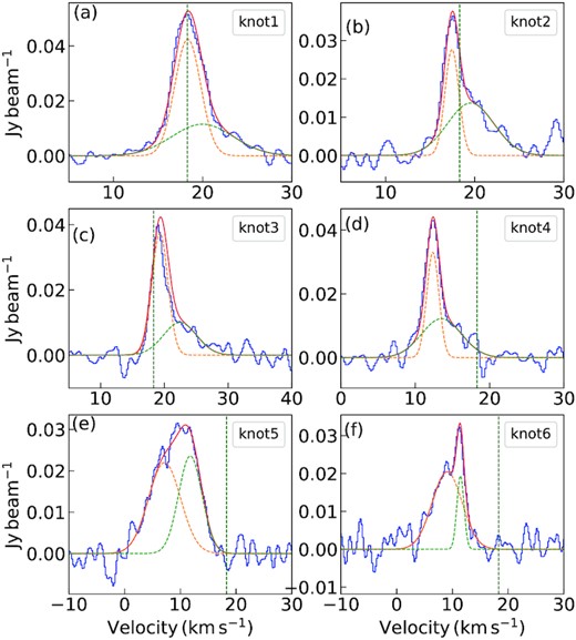
Averaged spectra of six positions marked by black circles in Fig. 14(a) presenting the outflow emission traced by different tracers towards G12.42. The SiO (2−1) spectra obtained using combined 12-m + 7-m data are drawn in blue lines. The spectra are boxcar smoothed by four channels resulting in a velocity resolution of 0.84|$\, \rm km\, s^{-1}$|. The orange and green dashed lines indicate the decomposed components of SiO (2−1) line and red spectral line is the resultant double Gaussian fitting. The vertical green dashed line marks the systemic velocity (18.3|$\, \rm km\, s^{-1}$|).
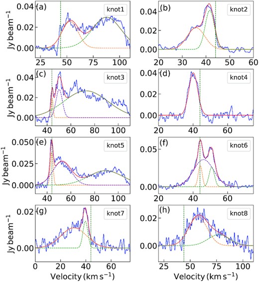
Averaged spectra of eight positions marked by black circles in Fig. 15(a) showing the outflow emission traced by different tracers towards G19.88. The SiO (2−1) spectra obtained using combined 12-m + 7-m data are drawn in blue lines. The spectra are boxcar smoothed by four channels resulting in a velocity resolution of 0.84|$\, \rm km\, s^{-1}$|. The orange, purple, and green dashed lines indicate the decomposed components of SiO (2−1) line and red spectral line is the resultant multi-Gaussian fitting. The vertical green dashed line marks the systemic velocity (44.0|$\, \rm km\, s^{-1}$|).
7 GRAVITY OR TURBULENCE: DECIPHERING THE DRIVING MECHANISM FOR MASSIVE STAR FORMATION IN THE PROTOCLUSTERS
Understanding the formation mechanism of massive stars has been one of the major focus areas of stellar astrophysics in the last decades or so. Together with the manyfold improvement in the observational data base, theoretical models including the core-accretion (McKee & Tan 2003; Krumholz et al. 2005, 2006) and the competitive-accretion (Bonnell et al. 2001, 2004) hypotheses have played a key role in unravelling the complex formation processes involved. The core-accretion theory presents a scaled-up version of the well-established theory of low-mass star formation. Here, massive stars form from pre-stellar cores, that are supported by turbulence or the magnetic field, via enhanced disc accretion. While successfully addressing the ‘radiation pressure’ problem, it leaves much to debate about the collapse time-scales and fragmentation of the massive pre-stellar cores. The competitive-accretion model, on the other hand, proposes fragmentation of clumps to low-mass cores and that the central cores chaotically gather mass by competing for it from intraclump gas reservoir. In addition to these pioneering theories, there are the current set of hierarchical fragmentation-based models for massive star formation. The two widely studied ones are the inertial-inflow (IF; Padoan et al. 2020) and the GHC (Vázquez-Semadeni et al. 2019) models. The IF model advocates for large-scale converging inertial inflow, driven by supersonic turbulence, to channel mass on to the accreting massive star. As proposed by these authors, the mass reservoirs are not controlled by gravity and global collapse is not necessary given the occurrence of turbulence driven compression at all scales. The GHC model proposes a very different uniform framework in which chaotic gravity-driven motions dominate at all scales. This is similar to the hierarchical Hoyle-like gravitational fragmentation taking place in the cloud where non-linear density fluctuations are formed by the initial turbulence. The conflicts and similarities of these hierarchical fragmentation models with the core-accretion and competitive-accretion models have been extensively discussed in Padoan et al. (2020) and Vázquez-Semadeni et al. (2019).
The detailed analysis of the ATOMS data gives a better insight regarding the interplay between gravity and turbulence in driving star formation in the two protoclusters studied here. Large-scale filamentary gas inflow is seen converging towards the central hub in protocluster G12.42 and evidence of a filamentary structure is also observed in G19.88. These filaments could be a natural manifestation of supersonic turbulence which finds support in the gas motion of the next spatial scale structure, the branches. These supersonic density structures are consistent with Larson’s velocity–size scaling presenting similar power-law exponent (∼0.5). While this supports the IF model, one cannot rule out the possibility of a gravity-driven mode in the filamentary flows which could be coupled to the turbulence cascade. Dissipation of turbulence at ∼0.1 pc is observed where the smaller scale structures show transonic or subsonic gas motions. Beyond this, the leaf structures deviate from Larson’s relation, showing a steeper slope. In conjunction with the virial analysis of the detected cores, where gravitational contraction is inferred from the low virial parameters derived, one can conjecture the onset of turbulence decoupling and dominance of gravitational acceleration towards the collapsing cores. The fragmentation analysis lends support to turbulence not being the key player driving clump to core fragmentation. Furthermore, Krumholz, McKee & Klein (2005) have shown that competitive-accretion could be a viable mechanism to form massive stars if the clumps that feed the accreting star are characterized by low virial parameters (αvir < 1). Similar low values of αvir are estimated for the dust clumps associated with the protoclusters. The predictions of the competitive accretion model are also argued to be consistent with that of the GHC model (Vázquez-Semadeni et al. 2019). Furthermore, a large population (more than 60 per cent) of the detected cores have masses ≲ MJeans, lending further support to the competitive accretion and the GHC scenario (Sanhueza et al. 2019). From the analysis presented, it is difficult to favour one model over the other. Based on the GHC and IF models, the overall observed picture of massive star formation could be a result of the scale-dependent combined effect of turbulence and gravity, which dominate on large and small scales, respectively. From the results presented here and in Liu et al. (2022a, b), the need for similar case studies is evident. Probing a large number of star-forming regions would enable us to obtain a better insight on the scale-dependent contribution of gravity and turbulence to the processes involved in high-mass star formation. Another key ingredient is the magnetic field. A complete understanding of these three crucial components is required to decipher the intricacies of massive star formation.
8 CONCLUSIONS
We have carried out a detailed continuum and multispectral line study of the region associated with the protoclusters G12.42+0.50 and G19.88−0.53 using data from the ATOMS survey. The main results are summarized below:
The continuum maps reveal the presence of seven cores in each of the two protoclusters. Every core qualifies as a massive star forming core satisfying the mass–radius relation and the surface mass density threshold. The observed dearth of low-mass cores implies the influence of stellar feedback on the process of fragmentation.
The global collapse scenario of the associated clumps has been addressed. Though previously identified as an infall candidate based on the nature of single dish line profiles, the ATOMS data of G12.42 show the presence of two distinct velocity components. However, several cores display characteristic infall signatures in the |$\rm HCO^+$| line profiles supported by single peak |$\rm H^{13}CO^+$| spectra. For G19.88, an infall signature is observed from the |$\rm HCO^+$| and |$\rm H^{13}CO^+$| line profiles. The virial analysis yields low values of the virial parameter (αvir << 2) indicating gravitational collapse in both protoclusters.
From the estimates of Jeans parameters (mass and length) and the observed range of mass and separation of the cores, we infer that turbulence does not drive the fragmentation of the clumps and thermal Jeans fragmentation adequately explains the process.
Gas kinematics at different spatial scales has been investigated. JCMT |$\rm {}^{13}CO$| (3−2) data show large scale, converging filamentary gas inflow in the G12.42 complex. For G19.88, such high quality CO molecular line data are required in the future to probe the gas motion in the associated filaments.
From the dendrogram analysis of the optically thin |$\rm H^{13}CO^+$| transition, several multiscale density structures (branches and leaves) are detected. The characteristic sizes (median values) are 0.1 and 0.03 pc for the branches and leaves, respectively. Combining the two protoclusters, 20 larger scale branch structures and 34 smaller scale leaf structures are identified. Analysis of the velocity variation, δV and the non-thermal velocity dispersion, σnt shows that the gas motion in the branch structures is supersonic and the leaves are mostly subsonic. The transition from the supersonic to the transonic regime occurs at spatial scales of ∼0.1 pc consistent with the scale at which dissipation of turbulence sets in.
Consistent with the above result, in the δV – L and σnt – L plots, the branches follow the canonical Larson’s relation and the leaves display a deviation (steepening) from it.
The smallest scale structure, the cores are likely to be in strong gravitational collapse as inferred from the low values of their virial parameters. In addition, several cores display the characteristic infall profiles with mass infall rates (∼1–7|$\times 10^{-3}\, \rm M_{\odot } yr^{-1}$|) being consistent with those found in other high-mass star-forming cores. Using SiO and |$\rm HCO^+$| molecular lines, multiple outflows are identified, which are likely to be driven by MM3 (49|$\, \rm M_{\odot }$|) in G12.42 and MM2 (23|$\, \rm M_{\odot }$|) in G19.88. In G19.88, an additional outflow is also identified using the |$\rm H^{13}CO^+$| line.
Based on the fragmentation analysis, the gas kinematics at various spatial scales, and the predictions of the IF and GHC models, the results obtained from this study indicate that the scale-dependent combined effect of turbulence and gravity is driving the formation of massive stars in the protoclusters.
The results of this study impel us to strongly advocate for more detailed case studies to address the exact behaviour of fragmentation and gas kinematics in protoclusters. EGOs associated with filamentary IRDCs present a sample of promising candidates as they are likely to be protoclusters harbouring stars with different masses and at different stages of evolution (Issac20 and references therein). These would provide a strong data base for considering scale-dependent contribution of turbulence and gravity in theories of massive star formation.
ACKNOWLEDGEMENTS
We thank the referee for the valuable suggestions that helped to improve the manuscript. HLL is supported by National Natural Science Foundation of China (NSFC) through the grant No.12103045. TL acknowledges the supports by National Natural Science Foundation of China (NSFC) through grants No.12073061 and No.12122307, the international partnership program of Chinese Academy of Sciences through grant No.114231KYSB20200009, Shanghai Pujiang Program 20PJ1415500 and the science research grants from the China Manned Space Project with no. CMS-CSST-2021-B06. CWL is supported by the Basic Science Research Program through the National Research Foundation of Korea (NRF) funded by the Ministry of Education, Science and Technology (NRF-2019R1A2C1010851), and by the Korea Astronomy and Space Science Institute grant funded by the Korea government (MSIT) (Project No. 2022-1-840-05). AS, GG, and LB gratefully acknowledge support by the ANID BASAL projects ACE210002 and FB210003. AS also acknowledges funding support through Fondecyt Regular (project codes 1180350 and 1220610) and from the Chilean Centro de Excelencia en Astrofísica y Tecnologías Afines (CATA) BASAL grant AFB-170002. This research was carried out in part at the Jet Propulsion Laboratory, which is operated by the California Institute of Technology under a contract with the National Aeronautics and Space Administration (80NM0018D0004). SLQ is supported by the National Natural Science Foundation of China (grant No. 12033005). KW acknowledges support by the National Key Research and Development Program of China (2017YFA0402702, 2019YFA0405100), and the National Science Foundation of China (11973013, 11721303). CE acknowledges the financial support from grant RJF/2020/000071 as a part of Ramanujan Fellowship awarded by Science and Engineering Research Board (SERB), Department of Science and Technology (DST), Government of India. This paper makes use of the following ALMA data: ADS/JAO.ALMA#2019.1.00685.S and #2017.1.00377.S. ALMA is a partnership of ESO (representing its member states), NSF (USA), and NINS (Japan), together with NRC (Canada), MOST and ASIAA (Taiwan), and KASI (Republic of Korea), in cooperation with the Republic of Chile. The Joint ALMA Observatory is operated by ESO, AUI/NRAO, and NAOJ. This research made use of astrodendro, a python package to compute dendrograms of Astronomical data (http://www.dendrograms.org/). This research made use of astropy, a community-developed core python package for Astronomy (Astropy Collaboration, 2018).
DATA AVAILABILITY
The data underlying this article will be shared on reasonable request to the corresponding author.
Footnotes
astrodendro is a pthyon package for computing dendrograms of astronomical data (http://www.dendrograms.org/)
