


ABSTRACT
Many dark matter (DM) models that are consistent with current cosmological data show differences in the predicted (sub)halo mass function, especially at sub-galactic scales, where observations are challenging due to the inefficiency of star formation. Strong gravitational lensing has been shown to be a useful tool for detecting dark low-mass (sub)haloes through perturbations in lensing arcs, therefore allowing the testing of different DM scenarios. However, measuring the total mass of a perturber from strong lensing data is challenging. Overestimating or underestimating perturber masses can lead to incorrect inferences about the nature of DM. In this paper, we argue that inferring an effective slope of the DM density profile, which is the power-law slope of perturbers at intermediate radii, where we expect the perturber to have the largest observable effect, is a promising way to circumvent these challenges. Using N-body simulations, we show that (sub)halo populations under different DM scenarios differ in their effective density slope distributions. Using realistic mocks of Hubble Space Telescope observations of strong lensing images, we show that the effective density slope of perturbers can be robustly measured with high enough accuracy to discern between different models. We also present our measurement of the effective density slope |$\gamma =1.96\substack{+0.12 \\ -0.12}$| for the perturber in JVAS B1938+666, which is a 2σ outlier of the cold DM scenario. More measurements of this kind are needed to draw robust conclusions about the nature of DM.
1 INTRODUCTION
Cosmological observations and galaxy dynamics have showed us that about 84 per cent of all matter in the Universe is composed of dark matter (DM), whose presence can be inferred via its gravitational influence. However, the Standard Model of particle physics lacks a description of it. The nature and interactions of DM remain one of the greatest puzzles of fundamental physics in modern times.
The standard cold dark matter (CDM) paradigm predicts that DM is clustered into gravitationally bound systems called haloes. These haloes are expected to roughly follow a power-law spectrum from galaxy clusters to ultra-faint dwarf galaxies (Davis et al. 1985; Navarro, Frenk & White 1996b, 1997; Moore et al. 1999; Green, Hofmann & Schwarz 2004; Wang et al. 2020). While the CDM model provides a good description of the Universe at large cosmological scales (Springel, Frenk & White 2006; Gil-Marín et al. 2016; Abbott et al. 2018; Abolfathi et al. 2018; Troxel et al. 2018; Planck Collaboration VI 2020), smaller scales remain largely untested. Moreover, many theoretical models describing the microphysics of DM disagree with CDM at small scales (Bode, Ostriker & Turok 2001; Kaplinghat 2005; Anderhalden et al. 2013; Lovell et al. 2014; Bullock & Boylan-Kolchin 2017; Buckley & Peter 2018; Tulin & Yu 2018).
Strong gravitational lensing is a promising observable that can be used as a probe of DM fluctuations at all scales, in particular those below that of the typical dwarf galaxies. Furthermore, in the coming years, we expect to have an increase in observed lensed systems, with tens of thousands expected to be discovered with upcoming optical imaging surveys (Collett 2015; Bechtol et al. 2019; Jacobs et al. 2019; Huang et al. 2021).
The (sub)halo mass function, which is the number of DM (sub)haloes as a function of mass, is commonly used to probe DM scenarios, in particular its low-mass end, where many theoretical DM models predict a suppression in the number of expected subhaloes or haloes along the line of sight (Angulo, Hahn & Abel 2013; Schneider 2015). So far, there have been a handful of claimed detections of low-mass substructure in strong lens systems (Vegetti et al. 2010, 2012; Hezaveh et al. 2016b) through perturbations in lensed arcs, as well as line-of-sight haloes (Şengül et al. 2022). The lack of detection of (sub)haloes together with the few detections have been used to constrain the properties of DM (Vegetti et al. 2014; Ritondale et al. 2019). At smaller physical scales where direct detection is not possible, the power spectrum of the collective perturbations of low-mass perturbers in the convergence field, either from subhaloes (Cyr-Racine et al. 2016b; Hezaveh et al. 2016a; Díaz Rivero et al. 2018b; Diaz Rivero, Cyr-Racine & Dvorkin 2018a; Brennan et al. 2019; Cyr-Racine, Keeton & Moustakas 2019) or line-of-sight haloes (Şengül et al. 2020), has been proposed as a powerful probe of CDM. The magnification ratio of multiple images has also been proposed as a probe of small-scale structure in the lens (Mao & Schneider 1998; Metcalf & Madau 2001) and has been used to detect subhaloes (Dalal & Kochanek 2002; Moustakas & Metcalf 2003; Amara et al. 2006; Fadely & Keeton 2011; Xu et al. 2012; MacLeod et al. 2013; Nierenberg et al. 2014, 2017) and line-of-sight haloes (Gilman et al. 2019). Additionally, the collective effects of the large population of low-mass (sub)haloes have been harnessed by machine learning techniques that attempt to extract information that may be buried in the observations (Brewer, Huijser & Lewis 2016; Daylan et al. 2018; Brehmer et al. 2019; Ostdiek, Diaz Rivero & Dvorkin 2022a, b; Wagner-Carena et al. 2022) as well as other types of techniques (Birrer, Amara & Refregier 2017).
When working with gravitational lensing as a probe, the total extended mass of a perturber is not an optimal parameter, since it relies on assumptions about the extended mass distribution (Vegetti et al. 2014; Vegetti & Vogelsberger 2014; Minor, Kaplinghat & Li 2017). Unusually dense perturbers will have a high lensing effect (despite their possible low mass), and vice versa. Hence, predicting the total mass from strong lensing measurements can be misleading. The substructure detected in the SDSSJ0946+1006 lens system (Vegetti et al. 2010) is a good example of these challenges. Its total mass (|$3.5 \times 10^{9}\, \mathrm{M}_\odot$|) was inferred by assuming a tidal truncation due to the host halo. Considering only its mass, this detection is consistent with predictions of CDM. However, a recent analysis (Minor et al. 2021b) of the subhalo has shown that this substructure is inconsistent with CDM with an unusually steep density slope. A robust way of measuring perturber masses has been proposed in Minor et al. (2017, 2021a) where they define a ‘perturbation radius’, which is the distance from the perturber to the critical curve in the direction in which the perturbation to the magnification is largest. The effective perturber lensing mass (this is, the projected mass within the perturbation radius, divided by the log-slope of the main lens’ 2D density profile) has been shown to be a robust estimator of the mass of the perturber under changes in the density profile (Minor et al. 2017). In addition to measuring the perturber mass, we can probe the density of the perturber as it falls with increasing radius. More specifically, the effect of perturbers in strong lensing systems is quite sensitive to the slope of the average convergence of the perturber at a characteristic scale, where we expect the effect of the perturber to have the largest observable effect. We call this the effective density slope. This effective slope is expected to vary under different DM scenarios, so a measurement of the effective slope would provide fertile grounds for discerning between different DM models.
Measuring the effective density slope may also shed light on a discrepancy claimed between the observations of dwarf galaxies and CDM simulations, known as the ‘cusp-core’ problem (Flores & Primack 1994; Moore 1994; de Blok et al. 2001; Gentile et al. 2004; de Blok 2010). The cusp-core problem refers to the fact that the observed central regions of galaxies (inferred from rotation curves) tend to have a lower amplitude and shallower slope of the density profile than the ones predicted from CDM simulations. When the effects of baryons are neglected, the CDM haloes show a self-similarity over a large mass range in simulations. These haloes can be approximated by the Navarro–Frenk–White (NFW) profile (Navarro et al. 1996b, 1997), with a ‘cusp’ at its centre, where the density (ρ) diverges with the distance r to the centre as ρ ∝ r−1. In contrast, the rotational speed of the stars in dwarf galaxies is observed to be roughly linear with radius, which implies a shallow inner slope, a ‘core’. The origin of this problem is yet unclear, and a number of solutions have been proposed to this problem, ranging from new physics in the form of warm dark matter (WDM) (Bode et al. 2001; Lovell et al. 2012), self-interacting dark matter (SIDM) (Spergel & Steinhardt 2000; Vogelsberger, Zavala & Loeb 2012; Rocha et al. 2013; Elbert et al. 2015), ultra-light DM (Hu, Barkana & Gruzinov 2000), or fluid DM (Peebles 2000) to the effect of baryons (Navarro, Eke & Frenk 1996a; Gnedin & Zhao 2002; Read & Gilmore 2005; Mashchenko, Couchman & Wadsley 2006; Brook et al. 2012; Governato et al. 2012; Pontzen & Governato 2012; Chan et al. 2015). A measurement of the effective density slope through gravitational lensing in dwarf galaxies should provide a powerful probe of CDM, since these systems are largely devoid of stars (Fitts et al. 2017; Read et al. 2017).
An observed diversity in rotation curves of dwarf galaxies has also been claimed to be poorly reproduced in simulations (Oman et al. 2015). This could be due to a limitation of numerical simulations in accounting for supernovae feedback or star formation mechanisms, or it could also be due to non-circular motions in the gas not accounted for (Marasco et al. 2018; Oman et al. 2018). Oman et al. (2015) show that systems for which the rotation curves do not agree with simulations also present a deficit in the enclosed mass compared to CDM simulations. They also show that for many of these systems the inner slopes are similar, while the rotation curves are very different. Different solutions in the form of DM self-interactions and baryonic flows have been suggested to solve this problem (Kaplinghat, Tulin & Yu 2016; Kamada et al. 2017; Kaplinghat, Ren & Yu 2020; Santos-Santos et al. 2020). However, these solutions each have shortcomings, hence it remains an open question.
In this work, we suggest the use of gravitational lensing to measure the power-law slope of the average convergence in an intermediate regime to discern between possible DM scenarios. This could help shed light on the problems mentioned above and give us new insights into the nature of DM. We will restrict our analysis to low-mass systems (≲109 M⊙), where the effect of baryons is expected to be small (Fry et al. 2015; Pereira Wilson et al. 2022).
This paper is organized as follows. In Section 2, we discuss how we determine the characteristic scale at which the power-law slope of a perturber is measured with lensing. In Section 3, we analyse the density profiles obtained from N-body simulations of different DM scenarios and extract their effective power-law slopes. We test the accuracy and robustness of the measurements of the effective power-law slopes of perturbers using realistic mocks of strong lensing images in Section 4. In Section 5, we present a measurement of the effective slope of the density profile of a perturber previously found in the strong lens system JVAS B1938+666. In Section 6, we summarize the results and the implications of our analysis. We include more details of our analysis in Appendices A, B, and C.
2 REGION OF MAXIMUM OBSERVABILITY
In general, our ability to probe the density profile of a perturber at very small radii is limited by resolution and noise. On the other hand, at much larger radii, the effect of the perturber is weaker and can be absorbed into the smooth model of the lens. Between these inner and outer radii, there is a region where we are most sensitive to the changes in the average convergence, which we will call the region of maximum observability (RMO). The effect on a lensing image of two perturbers with different density profiles is indistinguishable if they have overlapping average convergences within the RMO.
When modelling a gravitationally lensed image with a perturber, one has to simultaneously model the main lens, the external shear, and the source light. In general, it is not possible to measure the average convergence of a perturber without assuming it has some functional form. Only then, one can measure the parameters of that functional form. Determining the sensitivity of the images to the average convergence at various radii becomes tractable if we consider the much simpler problem of measuring a perturber from a noisy image when we know the main lens mass distribution, the perturber position, and the source-light distribution |$I_s(\vec{y})$|, where |$\vec{y}$| is a 2D vector representing the angular position on the lens plane. All the uncertainties we derive will therefore be lower bounds on the true uncertainties from modelling where all the lens and source parameters are varied.
In Fig. 1, we show an example of a result of this calculation, which assumes a PSF with a full width at half-maximum (FWHM) of 0.049 arcsec, a pixel size of 0.025 arcsec, a source with a Sersic profile, a main lens with an elliptical power-law (EPL) mass profile, and a perturber located near one of the bright images of the source created by the main lens. We see that for scales that are smaller than the pixel size, we are not able to measure the average convergence. This means that the very inner region (r < 0.04 arcsec) of any perturber placed on this location cannot be measured. For larger scales (r > 0.3 arcsec) the average convergence is again not well constrained since the effect of the perturber gets weaker as you get further from it. Between these two limits lies the RMO, where our errors are small enough to determine the profile of the perturber. However, because this region only spans roughly half a decade, an NFW perturber, which has a varying power-law slope, behaves effectively like a single power-law whose slope is the average slope of the true profile within the RMO.
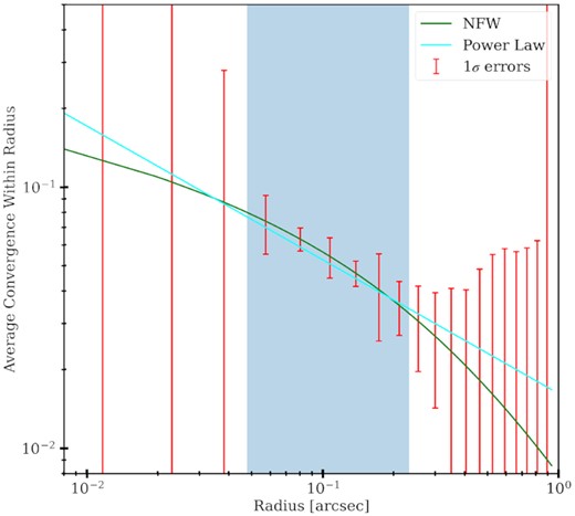
Sensitivity to the average convergence at various radii for an NFW perturber with |$M_{200} = 10^{9}\, \mathrm{M}_\odot$| and c200 = 12, where the main lens is at redshift z = 0.5 and the source is at z = 1.5. The green line shows the true NFW profile of the perturber. The cyan line shows the power-law best fit. The red error bars are the 1σ linear errors obtained from equation (8). The blue-shaded region shows the RMO, where the errors are less than twice the lowest one.
3 DENSITY PROFILE FOR DIFFERENT DM MODELS
In this section, we will analyse the density profile of high-resolution N-body simulations under different DM microphysics. The simulations used are the ETHOS (Effective Theory of Structure Formation) suite, originally presented in Vogelsberger et al. (2016) and Cyr-Racine et al. (2016a). In particular, five different DM scenarios are analysed: a CDM scenario and four other non-standard scenarios that include dark matter–dark radiation interactions, which produce a cut-off in the primordial power spectrum, and DM self-interactions, which affect the non-linear structure formation (under the label of ETHOS1-4). The parameters used in each simulation are described in Table 1. In particular, the parameters of the ETHOS4 simulation have been found to give a reasonable fit to observations of the Milky Way satellite population (Vogelsberger et al. 2016).
Relevant parameters of the ETHOS (Effective Theory of Structure Formation) models considered in this work. Here, αχ is the coupling between the mediator and dark matter, αν is the coupling between the mediator and a massless neutrinos-like fermion, mϕ is the mass of the mediator, and mχ is the mass of the DM particle. The parameter a4 is the coefficient of the power-law expansion in redshift of the DM drag opacity caused by the DM–DR interaction, which determines the linear initial matter power spectrum (see Cyr-Racine et al. 2016a). The parameters 〈σ〉30, 〈σ〉200, and 〈σ〉1000 are the DM self-interaction cross-sections at different velocities: 30, 200, and 1000 km s−1 and describe the velocity-dependent cross sections. We refer the reader to Vogelsberger et al. (2016) for more details on these models.
| Name | αχ | αν | mϕ [Gev c−2] | mχ [Gev c−2] | a4 [h Mpc−1] | 〈σ〉30/mχ [cm2 g−1] | 〈σ〉200/mχ [cm2 g−1] | 〈σ〉1000/mχ [cm2 g−1] |
|---|---|---|---|---|---|---|---|---|
| ETHOS1 | 0.071 | 0.123 | 0.723 | 2000 | 14095.65 | 4.98 | 0.072 | 0.0030 |
| ETHOS2 | 0.016 | 0.03 | 0.83 | 500 | 1784.05 | 9.0 | 0.197 | 0.00097 |
| ETHOS3 | 0.006 | 0.018 | 1.15 | 178 | 305.94 | 16.9 | 0.48 | 0.0028 |
| ETHOS4 | 0.5 | 1.5 | 5.0 | 3700 | 286.09 | 0.16 | 0.022 | 0.00075 |
For each DM scenario, we will extract the radial profiles of the perturbers in the simulation at different redshifts. In Fig. 2, we show an example of the normalized density profile of a CDM subhalo at redshift z = 1.47. We then calculate the average convergence of each profile as a function of radii, which is what the angular deflections of a perturber depend on. The power-law slope of the average convergence profile in the RMO (shown as the blue-shaded region in Fig. 2) is what we will call the effective power-law slope for each perturber. We should note that the RMO will be different for each perturber detected via strong lensing, depending on the resolution, main lens, source light, and the perturber position. Therefore, the RMO calculation needs to be done on a case-by-case basis. For the analysis in this section, we will assume that the main lens is at z = 0.88 and the source is at z = 2.079, as in the JVAS B1938+666 system. The rest of the properties of the main lens and the source are given by the best-fitting parameters of the JVAS B1938+666 lens system, as reported in Şengül et al. (2022).
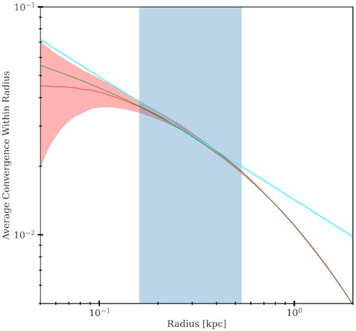
Illustrative example of the average convergence of a simulated CDM subhalo at z = 1.47 (in red line). The 1σ uncertainty due to the Poisson noise is shown as the red-shaded region. The subhalo follows a truncated NFW profile with concentration c200 = 12.7 and mass M200 = 4.3 × 10⁸M⊙ (the fit for the average convergence is shown in green line). The blue-shaded region shows the RMO within which we will be measuring the effective density slope in this work. The RMO depends on the configuration of the strong lensing system that the subhalo is perturbing. For this case, we assumed that it is placed in the JVAS B1938+666 system (which we describe in Section 5). The power-law best fit, which is only applied within the RMO, is shown in the cyan line.
We sort the particles of each perturber into radial bins and fit a power-law density profile (ρ ∝ r−γ) around the perturber radius to obtain the effective power-law slope, γ, for each perturber. We assume that the number of particles in each radial bin is a Poissonian realization of an underlying power-law density profile. The details of this analysis can be found in Appendix A. We only considered perturbers that are more massive than |$5\times 10^{7}\, \mathrm{M}_\odot$| to ensure that the radial bins are sufficiently populated to have an accurate effective power-law slope estimate. The particle mass of the simulations we use is |$2.8\times 10^{4}\, \mathrm{M}_\odot$|, which ensures that the smallest perturbers consist of more than 103 particles. We observe significant differences between the distribution of effective slopes in different DM scenarios. In Fig. 3, we show the effective density slope distributions of the different DM models at redshift z = 1.47. The CDM population has a mean of γCDM = 1.64 with a standard deviation of σ(γCDM) = 0.07. In the ETHOS1-4 models, the DM interactions with dark radiation and with itself result in a shallower profile. The ETHOS4 distribution has the largest overlap with CDM with a mean of γETHOS4 = 1.51 and a standard deviation of σ(γETHOS4) = 0.06.
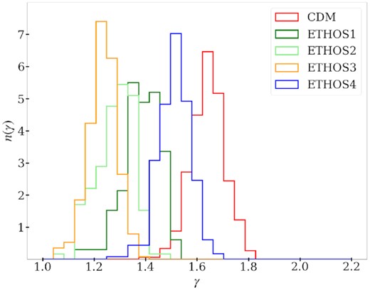
Normalized distributions of the effective density profile slopes (γ) of (sub)haloes with masses 5 × 10⁸ M⊙ < M < 2 × 10⁹ M⊙ for all five DM scenarios (CDM, ETHOS1-4) analysed in this work, at z = 1.47. The y-axis shows the fractional abundance of (sub)haloes. We see that the CDM population has the steepest mean effective slope.
We find a redshift dependence in the effective slope distributions of the different DM models, with a shift towards lower values of the slope as we increase the redshift. In Fig. 4, we show the distribution of γ for CDM, ETHOS3, and ETHOS4, at two redshifts. The mean γ of the CDM population shifts by 0.4σ (from γ = 1.67 to γ = 1.64 when going from z = 0.88 to z = 1.47, while the mean of the ETHOS4 distribution shifts by 0.6σ (from γ = 1.55 to γ = 1.51). The redshift dependence for ETHOS3 is stronger, which is expected since it has a higher DM self-interaction cross-section. The mean γ in the ETHOS3 model goes from γ = 1.29 at z = 0.88 to γ = 1.23 at z = 1.47, shifting by 1σ. This is likely due to the effect of tidal stripping (see the discussion below). This effect needs to be accounted for when using the effective density slope to probe different DM scenarios.
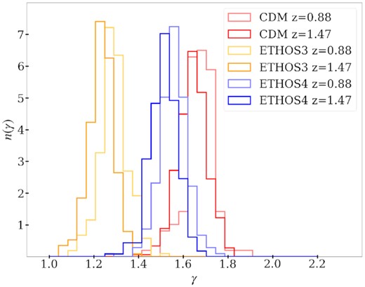
Redshift evolution of the normalized distributions of the effective density slopes (γ) of (sub)haloes with masses 5 × 10⁸M⊙ < M < 2 × 10⁹ M⊙ for CDM, ETHOS3, and ETHOS4. We see that for all scenarios the slope distributions shift towards lower values for higher redshifts.
In Fig. 5, we show the distribution of the masses and the effective power-law slopes of the perturbers at redshift z = 1.47 for two DM scenarios: CDM and ETHOS4. We note that lower masses have higher effective slopes on average. This mass dependence is stronger for CDM which makes the slope distributions at lower masses, with their means separated by ≈1.5σ for the case of CDM and ETHOS4. Due to the overlap in the distribution of slopes, we will not be able to distinguish between CDM and ETHOS4 with a single measurement. As we detect more and more perturbers, we will be able to determine from which underlying distribution the measured slopes are sampled.
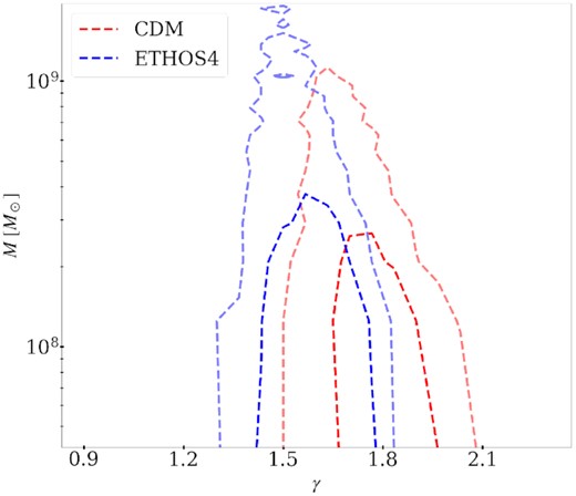
Distribution of mass versus the effective density profile slope of CDM (in red) and ETHOS4 (in blue) perturbers at redshift z = 1.47. The dashed contours enclose 68 per cent (darker colour) and 95 per cent (lighter colour) (which correspond to 1σ and 2σ) of the perturbers around the mean, respectively.
We further explore the distribution of the slopes and distances to the host centre for the subhaloes of the most massive halo in each set of simulations (in Fig. 6) and find a weak correlation between the two, most likely caused by the tidal forces of the host galaxy (Syer & White 1998). We find for all the models studied that the subhaloes that are closer to the centre of their host have lower slopes on average. This could be understood as follows: Tidal stripping can cause subhaloes to lose over 90 per cent of their total mass. During this mass-loss, the shape of the inner profile of the subhalo is preserved while the mass in the outer radii gets tidally stripped (Peñarrubia et al. 2010; Ogiya et al. 2019). A subhalo that ends up with a certain mass M after tidal stripping will have a larger scale radius compared to a subhalo with the same mass M that did not undergo tidal stripping, since the former started as a much more massive subhalo. Measuring the density slope within the same radii interval for both of these subhaloes will therefore give different values. For the tidally stripped subhalo, we will be probing the inner region of an originally more massive halo that lost its mass. These inner regions have a shallower density slope compared to the slope at larger radii. This correlation needs to be taken into account when using gravitational lensing measurements to discern between different DM scenarios.

Effective density profile slope (γ) versus the distance to the centre of the host halo of the subhaloes in the most massive haloes at each of the CDM, ETHOS3, and ETHOS4 simulations at redshift z = 0.88. The host halo has a total mass of |$M = 1.3 \times 10^{12}\, \mathrm{M}_\odot$| in each scenario.
4 MEASURING THE EFFECTIVE DENSITY SLOPE FROM HUBBLE SPACE TELESCOPE-LIKE NOISY MOCKS
We made realistic mock images of gravitational lenses at the resolution and sensitivity of Hubble Space Telescope (HST) observations to demonstrate the feasibility of measuring the effective density slope of perturbers. The images are 60 × 60 pixels with a pixel size of 0.025 arcsec, which gives a field of view of 1.5 arcsec × 1.5 arcsec. We assume a noise level of 10 HST orbits (33 000 s) of exposure and a Gaussian PSF with an FWHM of 0.049 arcsec. The sky brightness is 22.3 (AB magnitude) and the zero-point magnitude is 25.96.
We produced six mock images capturing possible variations in the models, which we list in Table 2 and show in Fig. 7. We set the lens redshift to z = 0.5 and the source redshift to z = 1.5 for all mock images. We analyse the mocks in this work using the publicly available code lenstronomy (Birrer, Amara & Refregier 2015; Birrer et al. 2021).
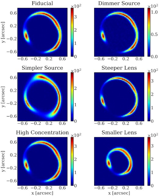
Mock images used in our analysis. The parameters of each image are described in Table 2.
The properties of each of the models analysed in this work (shown in Fig. 7). For the non-fiducial models we only list the parameters that differ from those of the fiducial. The remaining model parameters are chosen from uniform random distributions (see Appendix B for more details on the these models). The effective perturber lensing mass is kept fixed (at 1.5 × 10⁷ M⊙) in all the models (this is why the Steeper lens, High-concentration perturber, and Smaller lens models have a different value of M200). The effective perturber mass is the projected mass within the perturbation radius, divided by the log-slope of the main lens’ two-dimensional density profile (Minor et al. 2017).
| Model | Properties |
|---|---|
| Fiducial | θE, main = 0.55 arcsec |
| γmain = 2.0 | |
| |$M_\mathrm{200, perturber} = 10^{9}\, \mathrm{M}_\odot$| | |
| c200 = 12 | |
| mAB = 22 | |
| Nsersic = 5 | |
| Dimmer source | mAB = 24 |
| Simpler source | Nsersic = 1 |
| Steeper lens | γmain = 2.3 |
| |$M_\mathrm{200, perturber} = 1.27\times 10^{9}\, \mathrm{M}_\odot$| | |
| High-concentration perturber | c200 = 30 |
| |$M_\mathrm{200, perturber} = 1.93\times 10^{8}\, \mathrm{M}_\odot$| | |
| Smaller lens | θE, main = 0.35 arcsec |
| |$M_\mathrm{200, perturber} = 2.78\times 10^{9}\, \mathrm{M}_\odot$| |
We will now explain each of the cases analysed and refer the reader to Appendix B for more details on these models. We use dynesty (Speagle 2020), a publicly available nested sampling algorithm package, to sample the posterior probability distribution of the model parameters and to obtain the best fits from the sampled points. The main lens, external shear, and the perturber parameters are varied simultaneously during the posterior sampling. The means and standard deviations from the sampling as well as the true values for each case are shown in Table B1.
Fiducial model: For our fiducial case, we create a main lens with an Einstein radius of θE, main = 0.55 arcsec and a power-slope of γmain = 2.0. The x and y components of the centre of the main lens, the ellipticity of the main lens, and the external shear are all chosen randomly from uniform distributions in the range [−0.1 arcsec, 0.1 arcsec], [−0.1, 0.1], and [−0.1, 0.1], respectively. We place an NFW perturber with mass |$M_{200,\mathrm{perturber}} = 10^{9}\, \mathrm{M}_\odot$| and concentration c200 = 12 at (x, y) ≈ (0.212 arcsec, 0.465 arcsec) near a lensed arc of the source.
We model the source light with shapelets (Refregier 2003; Birrer et al. 2015, 2019; Shajib et al. 2020; Şengül et al. 2022), which are an orthonormal set of weighted Hermite polynomials. The source complexity is controlled by the shapelet-order parameter, nmax, that determines the number of degrees of freedom N via the relation N = (nmax + 1)(nmax + 2)/2. The size of the shapelet reconstruction is determined by the scaling parameter δ. Given a set of lens-model and shapelet parameters, the brightness of each pixel in the image is a linear function of the shapelet coefficients. If one knows the covariance matrix of the noise of the pixels, the best-fitting shapelet coefficients can be obtained by a simple matrix inversion. The centroid and the width of the shapelet basis are freely varied like any other model parameter. The optimal nmax changes depending on the complexity of the light distribution of the source galaxy and the resolution of the image. Therefore, we need to find the best fit nmax for each image on a case-by-case basis. We do this by starting from a low value of nmax = 5 and iterating by 1 until the Bayesian information criterion (BIC) of the best fit is larger than the previous iteration. The BIC is given by BIC = kln (n) + χ2, where k is the number of parameters in the model (this includes the number of shapelet coefficients) and n is the number of unmasked pixels.
We find that in the Fiducial model, we can measure a slope of |$\gamma = 1.559 \substack{+0.054 \\-0.035}$|. The posteriors of the perturber parameters are shown in Fig. 8(a). The average convergence profile of the power-law best fit is compared with the true NFW profile in Fig. 8(b) where we see that the best-fitting slope agrees with the average slope within the RMO. The red error bars are the 1σ linear errors we get on the average convergences at each radius when all other model parameters are fixed. We note that this fiducial case is encouraging since we can measure γ with an uncertainty of 3 per cent, which is smaller than the differences in the means of the different DM populations (which is at least 7 per cent, as shown in Fig. 3).
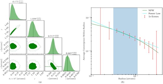
Fiducial model: (a) Posterior probability distribution of the perturber parameters. The true position values are shown in solid green lines. The average power-law slope in the RMO is shown as the dashed green line. (b) Average convergence as a function of radius. The power-law best fit for the Fiducial model is shown in the cyan line. The true NFW profile is shown with solid green lines. The red error bars show the 1σ linear errors of the average convergence within each radii. The blue-shaded region corresponds to the RMO.
Dimmer source: We analyse a case where the source is dimmer than the fiducial, with an AB magnitude of 24 instead of 22 (the amount of light we receive is reduced roughly by a factor of 6). We find, as expected, that the uncertainties of the model parameters are larger. The posteriors are shown in Fig. 9(a). We see in Fig. 9(b) that the RMO has shifted to larger radii compared to the fiducial case, due to the change in source brightness, which agrees with the steeper power-law measurement from modelling. Larger linear errors within the RMO mean that the pixel differences are consistent with a wider range of power-law slopes, which limits our capacity to measure the effective slope of the system. Source brightness is the most important factor that limits our capacity to probe the effective density slope of the perturbers.
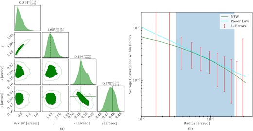
Dimmer source model: (a) Posterior probability distribution of the perturber parameters. The true position values are shown in solid green lines. The average power-law slope in the RMO is shown as the dashed green line. (b) Average convergence as a function of radius. The power-law best fit for the Dimmer source model is shown in the cyan line. The true NFW profile is shown with solid green lines. The red error bars show the 1σ linear errors of the average convergence within each radii. The blue-shaded region corresponds to the RMO.
Simpler source: If instead the source consists of a single Sersic profile instead of the five Sersics, we can measure the slope |$\gamma = 1.502 \substack{+0.05 \\-0.034}$|. We see that lowering source complexity does not change our ability to probe the effective power-law slope of the perturber. The posteriors are shown in Fig. 10(a). As we can see in Fig. 10(b), the RMO shifts towards smaller radii, which is consistent with our measurement of a shallower slope of the perturber.
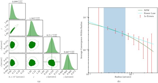
Simpler source model: (a) Posterior probability distribution of the perturber parameters. The true position values are shown in solid green lines. The average power-law slope in the RMO is shown as the dashed green line. (b) Average convergence as a function of radius. The power-law best fit for the Simpler source model is shown in the cyan line. The true NFW profile is shown with solid green lines. The red error bars show the 1σ linear errors of the average convergence within each radii. The blue-shaded region corresponds to the RMO.
Steeper lens: When the power-law slope of the matter distribution of the main lens is steeper (we increased it to 2.3), we measure a slope |$\gamma = 1.556 \substack{+0.059 \\-0.041}$| for the perturber. The uncertainty is slightly higher than that of the fiducial model, but the measurement is still precise enough to distinguish between the different DM scenarios analysed in this work. The posteriors are shown in Fig. 11(a). We find that the RMO does not get significantly affected by the change in the slope of the main lens, which can be seen by comparing Figs 8(b) and 11(b). Note that the perturber in this case has a larger M200, perturber compared to the fiducial one to keep the effective perturber lensing mass fixed.
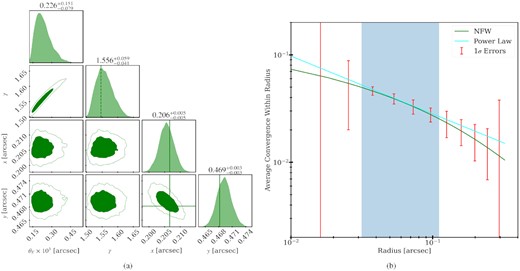
Steeper lens model: (a) Posterior probability distribution of the perturber parameters. The true position values are shown in solid green lines. The average power-law slope in the RMO is shown as the dashed green line. (b) Average convergence as a function of radius. The power-law best fit for the Steeper lens model is shown in the cyan line. The true NFW profile is shown with solid green lines. The red error bars show the 1σ linear errors of the average convergence within each radii. The blue-shaded region corresponds to the RMO.
High-concentration perturber: If the concentration of the perturber is raised to c200 = 30, we find that we can measure a slope of |$\gamma = 1.958 \substack{+0.074 \\-0.076}$|. The posteriors are shown in Fig. 12(a). Our slope measurement is consistent with the average slope within the RMO, which is not significantly affected by the change of the perturber profile, shown in Fig. 12(b). An NFW perturber with a higher concentration has a lower scale radius. Around the scale radius, the effective slope is roughly γ = 2. Since the RMO for this case (shown in Fig. 12b) includes the scale radius, which is rs ≈ 0.1 arcsec, we measure an effective slope close to 2. The best-fitting power-law is compared with the true NFW profile in Fig. 12(b). In this case, the perturber also has a larger M200, perturber compared to the fiducial one to keep the effective perturber lensing mass fixed.
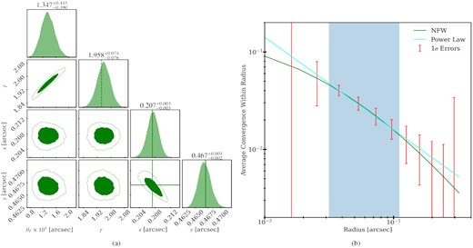
High-concentration perturber model: (a) Posterior probability distribution of the perturber parameters. The true position values are shown in solid green lines. The average power-law slope in the RMO is shown as the dashed green line. (b) Average convergence as a function of radius. The power-law best fit for the High-concentration perturber model is shown in the cyan line. The true NFW profile is shown with solid green lines. The red error bars show the 1σ linear errors of the average convergence within each radii. The blue-shaded region corresponds to the RMO.
Smaller lens: Furthermore, we tested making the Einstein radius of the main lens smaller (0.3 arcsec), and we found that in this case we can measure the slope |$\gamma = 1.465 \substack{+0.041 \\-0.032}$|. The posteriors are shown in Fig. 13(a). The slope is consistent with the expected one from the RMO, shown in Fig. 13(b). This case outperforms even the Fiducial model because, with a smaller Einstein radius, the source light (which is kept at the same magnitude) is now concentrated in a smaller number of pixels. Since we enforce that the perturber has to be close to those pixels, the deflections caused by the perturber are now measured more accurately. Another contributing factor is the perturber being more massive relative to the main lens (since now the latter has a smaller mass). The same perturber mass is now more dominant in the overall shape of the image. However, we note that in lenses with smaller Einstein radii, the probability of finding a perturber at bright enough positions is also smaller. Here again, the perturber has a larger M200, perturber value compared to the fiducial one to keep the effective lensing mass of the perturber fixed.
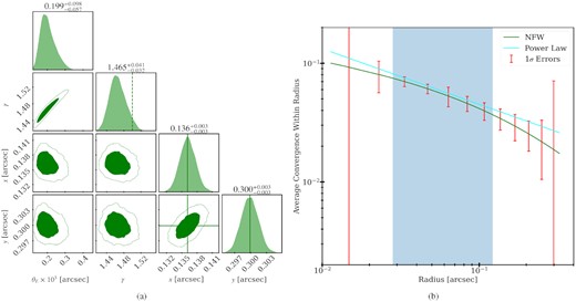
Smaller lens model: (a) Posterior probability distribution of the perturber parameters. The true position values are shown in solid green lines. The average power-law slope in the RMO is shown as the dashed green line. (b) Average convergence as a function of radius. The power-law best fit for the Smaller lens model is shown in the cyan line. The true NFW profile is shown with solid green lines. The red error bars show the 1σ linear errors of the average convergence within each radii. The blue-shaded region corresponds to the RMO.
4.1 Robustness tests
To confirm that we are indeed measuring the power-law slope of the average convergence within the RMO, we performed robustness tests where we create a set of mock lenses with an NFW perturber where the concentration of the perturber varies from c = 9 to c = 78, while the mass within the RMO is kept fixed at |$1.5\, \times \, 10^{7}\, \mathrm{M}_\odot$|. The choices we made for the rest of the lens parameters are the same as in the Fiducial case in Section 4. We expect to measure a steeper slope for the higher concentration case because an increase in concentration results in a decrease in the scale radius for an NFW halo. At the same scale, an NFW halo with a smaller scale radius has a steeper power-law slope than an NFW halo with a larger scale radius. In Fig. 14, we show the slope measurements as the green error bars obtained following the same modelling procedure described in Section 4, which involves sampling the posteriors of a model that has a power-law perturber. The cyan lines show the average power-law slope of the true NFW profile of each perturber within the RMO. We see that the measured slope agrees with the expected slope from the RMO for all the cases.

The expected and measured power-law slope for perturbers with varying concentration. The power-law slope of the average convergence within the RMO is shown in cyan line. The green error bars correspond to the 1σ confidence interval of the slope measurement obtained modelling the mock lens with a power-law perturber.
We have also tested for changes in the truncation radius, rt, of an NFW with a fixed mass and scale radius. We measure (again by modelling a mock lens with a power-law perturber) the effective slope of a truncated NFW perturber (Baltz, Marshall & Oguri 2009) with τ ≡ rt/rs = 1, 2, 3, 4, 5. In Fig. 15, we show with green error bars the 1σ confidence interval of the slope measurements from mock lenses by fitting a power law. The cyan line shows the average power-law slope of the true truncated NFW profile of each perturber within the RMO. For each case, we find that the measured slope matches the expected slope from the RMO.
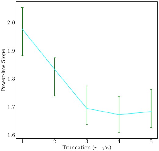
The expected and measured power-law slope for perturbers with varying truncation radius. The power-law slope of the average convergence within the RMO is shown in cyan line. The green error bars correspond to the 1σ confidence interval of the slope measurement obtained modelling the mock lens with a power-law perturber.
5 Measuring the effective density slope of the perturber in JVAS B1938+666
We will focus here on a perturber that has been previously detected in the strong lens system JVAS B1938+666 (Lagattuta et al. 2012; Vegetti et al. 2012), using the gravitational imaging technique (Koopmans 2005). The main lens in this system is at redshift z = 0.881 (Tonry & Kochanek 2000) and the source is at redshift z = 2.059 (Riechers 2011). The main lens has an Einstein radius of roughly θE ≈ 0.45 arcsec. We have reanalysed this system and found that the perturber that was previously assumed to be a subhalo is likely a line-of-sight halo. We refer to Şengül et al. (2022) for a detailed discussion of this analysis. In this section, we will present our measurement of the effective density slope of the perturber in JVAS B1938+666. In Vegetti et al. (2012), this perturber was shown to be consistent with a singular isothermal sphere (SIS) profile, which is a power law with a slope of γ = 2. A subsequent analysis (Vegetti & Vogelsberger 2014) found that for this system, a family of density profiles is consistent with an SIS profile over a large region in parameter space. Considering the sensitivity and the source-light distribution, they show that the data are not sensitive to the size of the inner density core. Motivated by these findings and our results in the previous section, we model the main lens and the perturber as an EPL, shown in equation (9), and an external shear. The perturber is modelled with a cylindrically symmetric power-law mass profile (by fixing q = 1 in equation 9). Although the true density profile of the perturber might deviate from this power-law at smaller and larger radii, the data are not currently sensitive to such deviations.
The source light is modelled with shapelets with an optimal shapelet index of nmax = 10. The shapelet index optimization is done by minimizing the BIC over models with different nmax, as in the previous section. The background and Poisson noise are set to match the noise level of the image used, following our previous analysis (Şengül et al. 2022).
We perform a likelihood analysis using dynesty (Speagle 2020), and show the posteriors of the perturber parameters in Fig. 16. The data, reconstruction, and residuals are shown in Appendix C. We find an effective density slope of |$\gamma =1.96\substack{+0.12 \\-0.12}$|. Assuming that the underlying slope distributions are Gaussian, our measurement is a >2.1σ outlier for a CDM slope distribution from simulations at z = 1.47 shown in Fig. 4. This result is also in 3.9σ, 4.5σ, 5.1σ, and 3.2σ tension with ETHOS1-4, respectively. If the perturber were a subhalo, instead of a line-of-sight halo as Şengül et al. (2022) shows, its slope would have to be compared to the z = 0.88 simulation snapshots. In this case the slope measurement would be a 1.9σ outlier for CDM and a 3.4σ, 4.1σ, 4.6σ, and 2.7σ outlier for the ETHOS1-4 models, respectively.
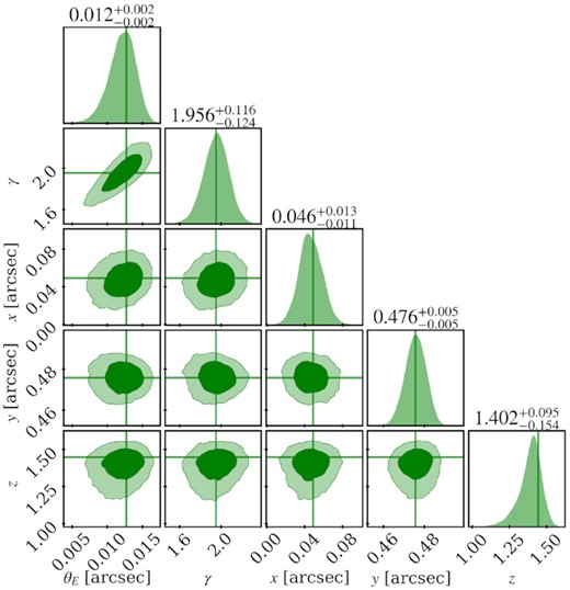
Posterior probability distribution of the perturber parameters in the system JVAS B1938+666. The vertical lines correspond to the best-fitting values of the parameters.
From our measurement of the power-law slope within the RMO and assuming that the mass distribution of the perturber follows an NFW profile, we can estimate the scale radius and the concentration of the perturber. Around the scale radius, the NFW profile slowly transitions from a slope of γ ≈ 3 to γ ≈ 1, as we move to smaller radii, as can be seen in Fig. 17. Therefore, the density profile of an NFW perturber that has a scale radius that is much smaller than the RMO will effectively behave like a power-law with a slope of γ ≈ 3. Conversely, when the scale radius is much larger than the RMO, the density profile of the perturber will behave like a power-law with a slope of γ ≈ 1. In our case, we are measuring a power-law slope of γ ≈ 2, which means that we are probing the density profile at roughly the NFW scale radius. In contrast to our previous study with mocks, for the real JVAS B1938+666 system, we do not know the true source-light distribution, main lens profile, and the perturber position. Instead, we use the best fits from our analysis of the system outlined in Şengül et al. (2022) to calculate the RMO. In Fig. 18, we show the linear errors for the average convergence of the perturber. The RMO is shown in the blue-shaded region. We see that we are most sensitive to the average convergence between roughly 0.04 and 0.13 arcsec. This corresponds to a physical scale of roughly |$0.17\!-\! 0.55\, \mathrm{kpc}$| at the redshift of the perturber. The scale radius of the perturber needs to be within the RMO so that the power-law slope of the perturber at our measurement scale is close to 2. If rs were any bigger (smaller), we would expect to measure a slope that is closer to γ = 1(3). Considering the measured mass of the perturber, a scale radius of |$r_s = 0.25 \, \mathrm{kpc}$| implies a concentration of roughly c200 ≈ 60, which is much higher than the expected value of c200 ≈ 10 given by the mass–concentration relation found in CDM simulations (Dutton & Macciò 2014). This is consistent with our measurement of |$c_{200} = 54 \substack{+21 \\-15}$| in Şengül et al. (2022) and also matches the expectation in Minor et al. (2021a) that only high-concentration perturbers with masses ≲109M⊙ are expected to be detected at the HST resolution.
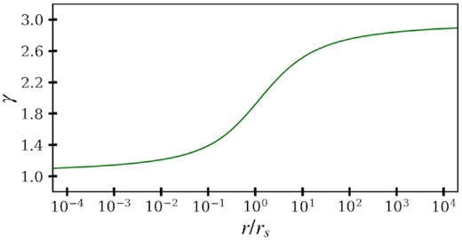
The effective slope of an NFW profile as a function of radius in units of the scale radius rs.
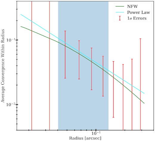
The linear errors for the perturber of the system JVAS B1938+666, calculated with the best fits of the main lens, shear, and source light from Şengül et al. (2022). The power-law best fit with γ = 1.95 is shown in cyan line. The NFW best fit is shown with the green line.
6 CONCLUSIONS
It is standard practice, in strong gravitational lensing studies, to provide a measurement of a system by making assumptions about its extended profile. In some cases, these assumptions can change the inferred mass by an order of magnitude, which can, in turn, prevent us from accurately probing the (sub)halo mass function, a derived quantity that is commonly used to distinguish between different DM scenarios. On the other hand, perturbations in strong lensing images due to low-mass subhaloes and line-of-sight haloes are quite sensitive to the power-law slope of the average convergence of the perturbers within an observable range (we call this the effective density slope in this work). We proposed in this work to use this effective density slope as a more direct parameter from strong gravitational lensing measurements, and we recommend future studies to report this parameter, as it will allow for a more accurate comparison with simulations of different DM scenarios.
Making predictions of structure formation at the relevant scales considered in this work is only possible by relying on simulations since structure formation is a highly non-linear process. For this purpose, we use the ETHOS zoomed-in simulations (Vogelsberger et al. 2016) of a Milky-Way-sized halo under different DM scenarios. We find that these scenarios show different distributions of effective density slopes of the DM perturbers, which can be used as a benchmark to test measurements of the density slopes of real perturbers. Although there is a significant overlap in the slope distribution of different scenarios, in general, CDM perturbers present a steeper slope compared to that of the more exotic DM scenarios (ETHOS1-4) analysed in this work. We also see that, for subhaloes, the slope is slightly correlated with its distance to the centre of the host. Subhaloes that are closer to their host, on average, have shallower effective slopes, populating the lower tails of the slope distributions in all the DM scenarios we considered.
We demonstrate the feasibility of measuring the effective density slope by making mock measurements of HST-like data. We find that if the source galaxy is sufficiently bright (an AB magnitude of 22 or brighter), measuring the slope of a perturber with a mass of |$1\times 10^{9}\, \mathrm{M}_\odot$| is possible with a |$3{{\ \rm per\ cent}}$| uncertainty. This measurement also depends on accurate modelling of the main lens profile. Deviations of the main lens mass distribution from an EPL can result in a bias in the inferred effective power-law slopes for perturbers. The differences in the means of the distributions observed in different DM populations are generally larger than our measurement accuracy, suggesting that we should be able to distinguish between different DM scenarios as we accrue more measurements of the slopes of the perturbers in strong lensing systems.
As a step towards this effort, we measure in this work the effective slope of the density profile of the perturber in the strong lens system JVAS B1938+666. We find that its slope is steeper than what is expected from simulations, being in strong tension with ETHOS1-3. It is also a ≈3σ outlier for ETHOS4 and a ≈2σ outlier for CDM. This tension can also be seen as a tension in concentration values. For an NFW halo, a steep slope indicates a high concentration and vice versa. More measurements of the slopes of perturbers are needed to tell if this indicates new physics, as perturbers with steeper effective slopes (higher concentrations) have a stronger lensing signal and are more likely to be detected.
In the upcoming years, we expect to find tens of thousands of new strong lensing systems with experiments such as the Vera C. Rubin Observatory, Euclid, the Dark Energy Survey (DES), the Dark Energy Spectroscopic Instrument (DESI), the Square Kilometre Array (SKA), and the Nancy Grace Roman Telescope (Oguri & Marshall 2010; Collett 2015; McKean et al. 2015; Huang et al. 2021). As the capabilities to observe strong lens systems increase, we expect to find a large number of perturbers. Follow-up analyses of these perturbers with high-resolution imaging from the HST, the James Webb Space Telescope, and the Extreme Large Telescope will provide us with a distribution of effective density slopes that can be then compared with simulations.
ACKNOWLEDGEMENTS
CD and ACS are partially supported by the Department of Energy (DOE) grant no. DE-SC0020223. We thank Mark Vogelsberger and Jesús Zavala for providing us with the CDM and ETHOS simulations analysed in this work. We would also like to thank Simon Birrer, Adam Coogan, Akaxia Cruz, Arthur Tsang, and Sebastian Wagner-Carena for valuable discussions.
DATA AVAILABILITY
The system analysed in this work is JVAS B1938+666. The data of this system are publicly available on https://mast.stsci.edu/portal/Mashup/Clients/Mast/Portal.html. The code used for our analysis is available at https://github.com/acagansengul/interlopers_with_lenstronomy. The data from the particle simulations will be shared on request to the corresponding author with permission of Mark Vogelsberger and Jesús Zavala.
REFERENCES
APPENDIX A: EXTRACTING THE AMPLITUDE AND SLOPE OF THE AVERAGE CONVERGENCE FROM SIMULATIONS
This appendix shows the details behind the extraction of the effective density slopes from N-body simulations.
APPENDIX B: ANALYSIS OF THE MOCK IMAGES
In this appendix, we show a complete list of the model parameters of the mock images analysed in Section 4. In Table B1, we show the mean and 1σ uncertainties of the lens-model parameters of the different cases listed in Table 2. We see that the means and the uncertainties of the main lens and shear parameters are consistent with the true values for all six cases considered here.
Lens-model properties of each of the models shown in Fig. 7. The first row of each model shows the true values, while the second row shows the means and standard deviations of the measurements coming from a likelihood analysis, as described in Section 4. The parameters cx and cy are the x and y coordinates of the centroid of the main lens, and exey are the x and y component of the ellipticity of the main lens profile. The true θE and γ for the perturbers are not applicable because they follow NFW profiles instead of EPL profiles.
| Model | Main lens | Shear | Perturber | |||||||||
|---|---|---|---|---|---|---|---|---|---|---|---|---|
| θE, main [arcsec] | γmain | cx × 103 [arcsec] | cy × 103 [arcsec] | ex × 103 | ey × 103 | Γx × 103 | Γy × 103 | θE × 103 [arcsec] | γ | x [arcsec] | y [arcsec] | |
| Fiducial | 0.550 | 2.0 | −40.0 | −12.1 | −31.5 | −59.8 | −78.4 | −92.6 | 0.189 | 0.481 | ||
| |${0.547}_{-0.002}^{+0.003}$| | |${2.00}_{-0.02}^{+0.02}$| | |${-40.1}_{-0.2}^{+0.2}$| | |${-12.3}_{-0.5}^{+0.5}$| | |${-31.6}_{-1.7}^{+1.7}$| | |${-60.2}_{-1.4}^{+1.4}$| | |${-78.3}_{-1.7}^{+1.8}$| | |${-92.3}_{-1.4}^{+1.5}$| | |${0.17}_{-0.05}^{+0.11}$| | |${1.559}_{-0.035}^{+0.054}$| | |${0.212}_{-0.004}^{+0.004}$| | |${0.465}_{-0.002}^{+0.003}$| | |
| Dimmer Source | 0.550 | 2.0 | −40.0 | −12.1 | −31.5 | −59.8 | −78.4 | −92.6 | 0.207 | 0.468 | ||
| |${0.548}_{-0.005}^{+0.005}$| | |${2.05}_{-0.06}^{+0.07}$| | |${-39.7}_{-1.0}^{+1.0}$| | |${-12.0}_{-1.5}^{+1.5}$| | |${-34.0}_{-6.6}^{+6.6}$| | |${-61.1}_{-5.5}^{+5.3}$| | |${-82.0}_{-5.3}^{+5.3}$| | |${-94.8}_{-4.4}^{+4.4}$| | |${0.51}_{-0.29}^{+0.71}$| | |${1.683}_{-0.102}^{+0.153}$| | |${0.194}_{-0.020}^{+0.027}$| | |${0.478}_{-0.012}^{+0.010}$| | |
| Simpler Source | 0.550 | 2.0 | −40.0 | −12.1 | −31.5 | −59.8 | −78.4 | −92.6 | 0.211 | 0.468 | ||
| |${0.546}_{-0.004}^{+0.004}$| | |${1.97}_{-0.02}^{+0.02}$| | |${-40.3}_{-0.4}^{+0.4}$| | |${-12.6}_{-0.6}^{+0.6}$| | |${-30.6}_{-1.7}^{+1.7}$| | |${-58.8}_{-2.2}^{+2.2}$| | |${-76.3}_{-1.4}^{+1.4}$| | |${-90.3}_{-1.5}^{+1.4}$| | |${0.10}_{-0.03}^{+0.07}$| | |${1.502}_{-0.034}^{+0.050}$| | |${0.211}_{-0.004}^{+0.005}$| | |${0.467}_{-0.004}^{+0.005}$| | |
| Steeper Lens | 0.550 | 2.3 | −40.0 | −12.1 | −31.5 | −59.8 | −78.4 | −92.6 | 0.207 | 0.468 | ||
| |${0.547}_{-0.002}^{+0.003}$| | |${2.30}_{-0.03}^{+0.03}$| | |${-40.1}_{-0.2}^{+0.2}$| | |${-12.3}_{-0.4}^{+0.5}$| | |${-31.9}_{-2.2}^{+2.2}$| | |${-59.7}_{-2.3}^{+2.1}$| | |${-78.2}_{-1.8}^{+1.7}$| | |${-91.9}_{-1.9}^{+1.7}$| | |${0.23}_{-0.08}^{+0.15}$| | |${1.556}_{-0.041}^{+0.059}$| | |${0.206}_{-0.005}^{+0.005}$| | |${0.469}_{-0.003}^{+0.003}$| | |
| High-concentration Perturber | 0.550 | 2.00 | −40.0 | −12.1 | −31.5 | −59.8 | −78.4 | −92.6 | 0.207 | 0.467 | ||
| |${0.549}_{-0.001}^{+0.001}$| | |${2.00}_{-0.02}^{+0.02}$| | |${-40.0}_{-0.2}^{+0.2}$| | |${-12.3}_{-0.4}^{+0.4}$| | |${-31.5}_{-1.7}^{+1.6}$| | |${-60.0}_{-1.4}^{+1.4}$| | |${-78.3}_{-1.6}^{+1.6}$| | |${-92.5}_{-1.3}^{+1.3}$| | |${1.35}_{-0.39}^{+0.44}$| | |${1.958}_{-0.076}^{+0.074}$| | |${0.207}_{-0.003}^{+0.003}$| | |${0.467}_{-0.002}^{+0.003}$| | |
| Smaller Lens | 0.350 | 2.00 | −40.0 | −12.1 | −31.5 | −59.8 | −78.4 | −92.6 | 0.136 | 0.300 | ||
| |${0.345}_{-0.004}^{+0.004}$| | |${2.00}_{-0.02}^{+0.02}$| | |${-40.0}_{-0.3}^{+0.3}$| | |${-12.2}_{-0.5}^{+0.5}$| | |${-32.3}_{-2.7}^{+2.7}$| | |${-59.0}_{-2.7}^{+2.7}$| | |${-77.8}_{-2.3}^{+2.4}$| | |${-90.7}_{-2.2}^{+2.1}$| | |${0.20}_{-0.06}^{+0.10}$| | |${1.465}_{-0.032}^{+0.041}$| | |${0.136}_{-0.003}^{+0.003}$| | |${0.300}_{-0.003}^{+0.003}$| | |
Degeneracy between main lens model and the perturber
We present in Fig. B1 the posterior probability distributions of the model parameters for the Fiducial case. We see a strong correlation between the Einstein radius of the main lens model (θE, main) and the effective power-law slope of the perturber (γ). This indicates that failing to correctly model the main lens mass profile can result in a biased measurement of the power-law slope for perturbers.

Source reconstruction
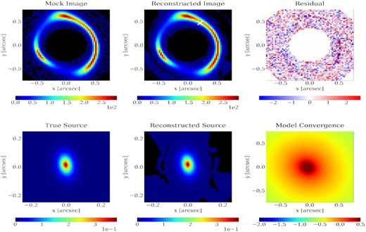
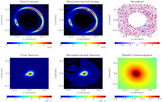
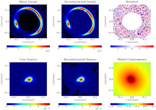
We present in Figs B2, B3, B4, B5, B6, and B7 the source used for the models analysed in Section 4, along with its reconstructions.

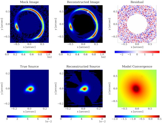
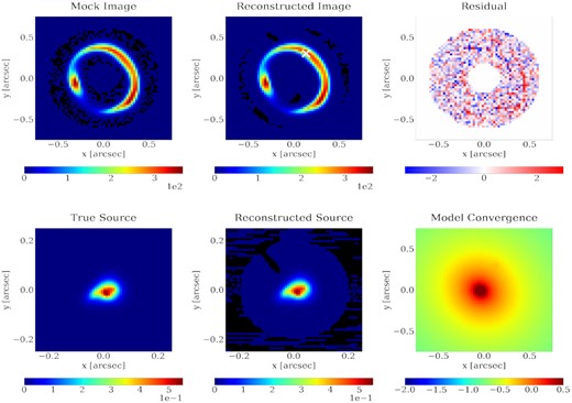
Best fit of the Fiducial mock in Table 2. The top left panel shows the mock image with noise. The top middle panel shows the model reconstruction from the best fit, where the perturber position is marked with the white cross. The top right panel shows the residuals divided by the noise in each pixel. The bottom left panel shows the true source distribution that is made up of five Sersic components. The bottom middle panel shows the shapelet reconstruction of the source. The bottom right panel shows the convergence of the best-fitting model in log scale, where the perturber can be seen as a small peak.
APPENDIX C: DATA, RECONSTRUCTION, AND RESIDUALS IN JVAS B1938+666
The HST image of JVAS B1938+666 used in this study, its reconstruction, and residuals are shown in Fig. C1. The posterior probability distributions of the model parameters obtained by nested sampling are shown in Fig. C2
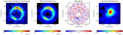
Lens-light-subtracted HST image of the lens JVAS B1938+666, the model prediction (where the mass profile of the perturber is modelled with a free power-law slope, as in Section 5), the residuals of the model with a perturber, and the reconstructed source (left- to right-hand panels).
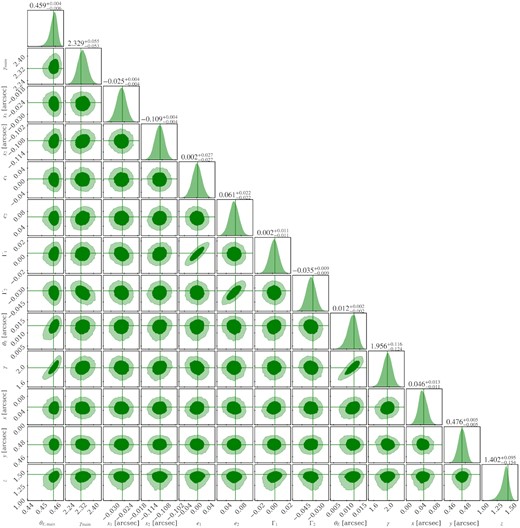
Posterior probability distribution of the model parameters in the system JVAS B1938+666. The parameters θE, main, γmain, x1, x2, e1, and e2 are the Einstein radius, power-law slope, the x and y coordinate of the centre, and the Cartesian ellipticity components of the main lens profile, respectively. The parameters Γ1 and Γ2 are the Cartesian components of the external shear. The parameters θE, γ, x, y, and z are the Einstein radius, the power-law slope, the x and y coordinate of the centre and the redshift of the perturber, respectively. The vertical lines correspond to the best-fitting values of the parameters.
