


ABSTRACT
Using high angular resolution ALMA observations (0.02 arcsec ≈ 0.34 pc), we study the thermal structure and kinematics of the proto-super star cluster 13 in the central region of NGC 253 through their continuum and vibrationally excited HC3N emission from J = 24−23 and J = 26−25 lines arising from vibrational states up to v4 = 1. We have carried 2D-LTE and non-local radiative transfer modelling of the radial profile of the HC3N and continuum emission in concentric rings of 0.1 pc width. From the 2D-LTE analysis, we found a Super Hot Core (SHC) of 1.5 pc with very high vibrational temperatures (>500 K), and a jump in the radial velocity (21 km s−1) in the SE-NW direction. From the non-local models, we derive the HC3N column density, H2 density, and dust temperature (Tdust) profiles. Our results show that the thermal structure of the SHC is dominated by the greenhouse effect due to the high dust opacity in the IR, leading to an overestimation of the LTE Tdust and its derived luminosity. The kinematics and Tdust profile of the SHC suggest that star formation was likely triggered by a cloud–cloud collision. We compare proto-SSC 13 to other deeply embedded star-forming regions, and discuss the origin of the |$L_\text{IR}/M_{\text{H}_2}$| excess above ∼100 L⊙ M|$_\odot ^{-1}$| observed in (U)LIRGs.
1 INTRODUCTION
Using high angular resolution ALMA observations (0.02 arcsec ≈ 0.34 pc), we study the thermal structure and kinematics of the proto-super star cluster 13 in the central region of NGC 253 through their continuum and vibrationally excited HC3N emission from J = 24−23 and J = 26−25 lines arising from vibrational states up to v4 = 1. We have carried 2D-LTE and non-local radiative transfer modelling of the radial profile of the HC3N and continuum emissions. From the 2D-LTE analysis, we found a Super Hot Core (SHC) with high vibrational temperatures (>500 K), and a jump in the radial velocity (21 km s−1) in the SE-NW direction. From the non-local models, we derive the HC3N column density, H2 density, and dust temperature (Tdust) profiles. The thermal structure of the SHC is dominated by the greenhouse effect leading to an overestimation of the LTE Tdust and the corresponding luminosities. Star formation seems to be centrally peaked, supporting the competitive accretion scenario. The formation of the super star cluster was most likely triggered by a cloud–cloud collision as suggested by the kinematics of the SHC. Finally, we compare proto-SSC 13 to other deeply embedded star-forming regions, and discuss the origin of the |$L_\text{IR}/M_{\text{H}_2}$| excess above ∼100 L⊙ M|$_\odot ^{-1}$| observed in (U)LIRGs.
Even though a large number of SSCs have been observed in different starbursting galaxies (e.g. Melnick, Moles & Terlevich 1985; Whitmore et al. 1993; O’Connell, Gallagher & Hunter 1994; Meurer et al. 1995; Whitmore & Schweizer 1995; Ho & Filippenko 1996b, a; Watson et al. 1996; Whitmore et al. 1999; Gelatt, Hunter & Gallagher 2001; Tremonti et al. 2001; Vanzi 2003; Turner & Beck 2004; McCrady, Graham & Vacca 2005; Melo et al. 2005; Mengel et al. 2008), most of these studies have been carried out in the UV, optical, or near-IR wavelengths (see Portegies Zwart, McMillan & Gieles 2010, for a review), detecting relatively evolved SSCs. This is because SSCs remain entirely enshrouded by the large column densities of their natal giant molecular cloud during their formation and earliest phases of evolution, preventing the direct observations of these stages at the aforementioned wavelengths. Therefore, little is known about SSCs during their early evolutionary phases apart from the fact that they need to form most of the stars in a very short time-scale before the feedback from massive stars starts to disrupt and disperse the natal cloud (supernovae from the most massive stars take place after ∼105 yr of stellar evolution; Bressert et al. 2012; Krumholz et al. 2014), requiring relatively high star formation rates (SFRs) (Beck 2015).
Thanks to ALMA and its high angular resolution and sensitivity, we can now observe high energy molecular lines in the (sub)millimetre range, sampling the hot molecular environments within the obscuring dust regions. This allow us to study the embedded phase of proto-SSCs during their super hot core phase (SHC), a scaled-up version of galactic molecular hot cores (see Rico-Villas et al. 2020). The rotational transitions from vibrationally excited states of HC3N and HCN, usually excited by mid-IR (e.g. González-Alfonso & Sakamoto 2019), are excellent tracers of the SHC phase. Since HC3N has a much lower rotational constant (Bν ∼ 4.5 GHz) than HCN does (Bν ∼ 44.4 GHz) and allows up to seven normal vibrational modes (four stretching modes: v1, v2, v3, v4; and three bending modes: |$v_5,\, v_6,\, v_7$|), it has more rotational transitions in a given wavelength range (1 every ∼9 GHz), covering a wider energy range. With such many rotational lines from different vibrationally excited states, we are able to study the thermal structure and the kinematics of proto-SSCs with unprecedented detail. This provides the only way to estimate the stellar content in the earliest evolutionary phases of SSCs (proto-SSCs) through the determination of the luminosity of the SHC phase. However, as discussed by Rico-Villas et al. (2020, 2021), the determination of the luminosity from vibrationally excited HC3N (hereafter HC3N*) emission is not straightforward due to the back-warming of radiation (Donnison & Williams 1976; Rowan-Robinson 1982; Ivezic & Elitzur 1997). This greenhouse effect produced by the back-warming (González-Alfonso & Sakamoto 2019) is caused by the high column densities (≳ 1025 cm−2) and thus high dust opacities, which increase the inner dust temperatures well above the expected dust temperature in the optically thin case. This effect, by increasing the dust temperature and the mid-IR (wavelength responsible for the vibrational excitation of HC3N) radiation field in the innermost regions, leads to an overestimation of the luminosity of the SHCs. To fully account for this effect and to derive reliable luminosities, the inner thermal structure needs to be derived from spatially resolved observations of the HC3N* emission.
Such study was done in Rico-Villas et al. (2020) at a resolution of 0.29 arcsec × 0.19 arcsec (|$4.9\, \text{pc}\times 3.2\, \text{pc}$|) for the 14 forming SSCs previously analysed by Leroy et al. (2018) in the nuclear region of the galaxy NGC 253. This galaxy, located at 3.5 Mpc,1 is one of the closest galaxies hosting a nuclear starburst (for details see Mills et al. 2021). Through the detection of HC3N* in the v7 = 1, v7 = 2, and v6 = 1 states, Rico-Villas et al. (2020) estimated the luminosity and age of the SSCs in the nuclear region. The high luminosities and young ages proved that they were forming stars at high rates with high star formation efficiencies (SFEs).
In this work, thanks to new ALMA observations at an order of magnitude higher angular resolution of 0.022 arcsec × 0.020 arcsec (|$0.37\, \text{pc}\times 0.34\, \text{pc}$|), we are able to resolve most of the forming SSCs studied in Rico-Villas et al. (2020) and study in detail the inner thermal structure and kinematics from HC3N* emission in the proto-SSC 13. We selected to study this source in detail because it has one of the brightest continuum emission, was among the youngest sources in Rico-Villas et al. (2020), and has no clear outflow signatures (Levy et al. 2021). We combine the continuum data (at 219 and 345 GHz) and the HC3N* line emission with non-local radiative transfer models (which include all the high vibrationally excited states detected), to obtain the temperature and density profiles of a proto-SSC, and confirm the presence of the back-warming effect as expected from the high column densities. We also establish that the IR luminosities derived from the HC3N* emission are overestimated by about an order of magnitude if the greenhouse effect is ignored.
2 OBSERVATIONS
We observed the nuclear region of NGC 253 using the ALMA 12 m Array at very high angular resolution. We performed Band 6 (211–275 GHz coverage) observations in ALMA configuration C43-9 (ALMA project 2018.1.01395.S, PI: Rico-Villas, Fernando), which provides the required high angular resolution to resolve most of the proto-SSCs studied in Rico-Villas et al. (2020). In order to observe the maximum number of HC3N* lines as possible, we optimized the correlator set up by tuning the Local Oscillator at 227.889 GHz, allowing us to record in the lower and upper side bands the frequencies of the J = 24 − 23 (∼220 GHz) and J = 26 − 25 (∼237 GHz) HC3N* rotational transitions. The four spectral windows, with a bandwidth of 1.875 GHz and a channel resolution of 1.3 km s−1, were tuned to cover the frequencies 218.16–220.03 GHz and 220.01–221.88 GHz for the lower side band, and 234.32–236.19 GHz and 236.17–238.04 GHz for the upper side band.
The observations were carried out in six different execution blocks between 2019 June and 2019 July, with an average exposure time on source per execution block of 44.45 min, and a total integration time of 4.45 h. During the observations, short scans of J0006–0623 were used for bandpass and flux calibration; J0038–2459 was used for phase calibration. A summary of the observation details can be found in Table 1. The table shows the shortest baselines for each execution block, which set the maximum recoverable scale (MRS2) between 0.35 and 0.38 arcsec (5.9 and 6.4 pc). This MRS should be enough to assume that the entire flux all the compact SHCs (with sizes |$\lt 2\, \text{pc}$|; Rico-Villas et al. 2020) is recovered. To obtain further information about the dust emission, we used also Band 7 observations from the ALMA project ID: 2017.1.00433.S (PI: Bolatto, Alberto) at ∼345 GHz. For further details on this observations see Levy et al. (2021).
Log of ALMA Cycle 6 observations NGC 253.
| Date | N. Ant. | Short. Base. | Long. Base. | Int. Time |
|---|---|---|---|---|
| (UT) | (m) | (m) | (min) | |
| 2019-06-06 | 43 | 210 | 15 238 | 44.30 |
| 2019-06-08 | 42 | 83 | 16 196 | 44.43 |
| 2019-06-09 | 43 | 83 | 16 196 | 44.52 |
| 2019-06-10 | 47 | 83 | 16 196 | 44.48 |
| 2019-06-12 | 41 | 83 | 16 196 | 44.62 |
| 2019-07-10 | 41 | 138 | 13 894 | 44.38 |
2.1 Imaging
The visibilities were calibrated using the casa3 5.6.1-8 package (Common Astronomy Software Applications; McMullin et al. 2007) pipeline version 42866. For the imaging we then combined the visibilities of the six execution blocks using the tclean task from the same casa 5.6.1-8 version. For image cleaning we applied a Briggs weighting scheme, setting the robust parameter to 0.5. For masking we used the option auto-multithresh to automatically mask regions during the deconvolution (Kepley et al. 2020). The channel width was set to the original spectral resolution of 1 MHz (i.e. ∼1.3 km s−1). Considering the resulting angular resolution of ∼0.025 arcsec, we set the pixel size to 0.007 arcsec (0.12 pc) to have at least 9 pixels per beam solid angle (i.e. 1.5 times Nyquist sampling). After the imaging, we applied the primary beam correction. Due to the large number of emission and absorption lines expected towards the proto-SSCs, the spectral cubes were imaged from the visibilities without applying a uv-plane continuum subtraction. The resulting synthesized beams, channel resolution, covered frequencies, and rms for each spectral cube are listed in Table 2. For the spectral cubes, the continuum was subtracted by fitting order 0 baselines. A continuum map (Fig. 1) was generated from apparently line-free channels in the uv-plane with a synthesized beam of 0.020 arcsec × 0.019 arcsec (|$0.34\, \text{pc}\times 0.32\, \text{pc}$|) and a rms noise of 13 |$\mu $|Jy beam−1. However, due to the significant spectral feature contribution mentioned above, the continuum emission in these regions has to be treated with caution.
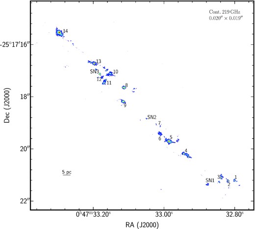
Continuum map at 219 GHz of the NGC 253 nuclear region with a resolution of 0.020 arcsec × 0.019 arcsec above 3σ219GHz (σ219GHz = 13 |$\mu $|Jy). Labelled are the proto-SSCs studied in Rico-Villas et al. (2020).
ALMA ID 2018.1.01395.S project NGC 253 reduced spectral cubes properties. The table lists the covered rest frequencies, the synthesized beam, position angle, channel width, and channel rms for each spectral cube.
| Rest Freq. | Syn. Beam | PA | Ch. width | rms |
|---|---|---|---|---|
| (GHz) | (arcsec2) | (|$\deg$|) | (km s−1) | (mJy beam−1) |
| 218.16–220.03 | 0.026 × 0.022 | 42 | 1.34 | 0.38 |
| 220.01–221.88 | 0.023 × 0.022 | 64 | 1.33 | 0.35 |
| 234.32–236.19 | 0.022 × 0.020 | 53 | 1.24 | 0.37 |
| 236.17–238.04 | 0.022 × 0.020 | 47 | 1.23 | 0.39 |
For the ∼345 GHz data reduction and calibration of the visibilities we used the casa 5.1.1-5 pipeline version 40896. For the imaging of the uv-plane continuum, we selected line emission free channels and used the tclean task with the robust parameter set to 0.5 and left the default pixel from the pipeline (i.e. 0.005 arcsec = 0.085 pc). The resulting continuum map at 345 GHz has a resolution of 0.028 arcsec × 0.034 arcsec (|$0.47\, \text{pc}\times 0.58\, \text{pc}$|) and a rms noise of 37 |$\mu $|Jy beam−1. A summary of the image details of the continuum maps used in this work is shown in Table 3.
NGC 253 continuum map images parameters.
| Project ID | Rest Freq. | Syn. Beam | PA | rms |
|---|---|---|---|---|
| (GHz) | (arcsec2) | (|$\deg$|) | (|$\mu $|Jy beam−1) | |
| 2018.1.01395.S | 219 | 0.020 × 0.019 | 70 | 13 |
| 2017.1.00433.S | 345 | 0.028 × 0.034 | 79 | 37 |
| Project ID | Rest Freq. | Syn. Beam | PA | rms |
|---|---|---|---|---|
| (GHz) | (arcsec2) | (|$\deg$|) | (|$\mu $|Jy beam−1) | |
| 2018.1.01395.S | 219 | 0.020 × 0.019 | 70 | 13 |
| 2017.1.00433.S | 345 | 0.028 × 0.034 | 79 | 37 |
3 THE SPATIAL STRUCTURE OF SSCS
The very high resolution ALMA data (|$\sim 0.40\, \text{pc}\times 0.35\, \text{pc}$|) at ∼220–235 GHz allows us to study in detail the structure and kinematics of the proto-SSCs analysed in Leroy et al. (2018) and Rico-Villas et al. (2020). The study carried out in Rico-Villas et al. (2020) was done at a resolution of 0.29 arcsec × 0.19 arcsec (|$4.9\, \text{pc}\times 3.2\, \text{pc}$|) at ∼219 GHz. At similar frequencies (218–238 GHz), this new data set provides a resolution up to one order of magnitude higher (|$0.026\,{\rm arcsec}\times 0.022\,{\rm arcsec }=0.44\, \text{pc}\times 0.38\, \text{pc}$|, see Table 2) than our previous analysis. Some of the 14 proto-SSCs studied in Rico-Villas et al. (2020) show clear inner structure with several components (SSCs 14, 13, 12, 11, 10, 8, 5, 4, 3, 1; see Fig. 1). This can be seen in the continuum map at 219 GHz in Fig. 1, encompassing all the proto-SSCs. The structure of the fragmented proto-SSCs is better illustrated in Fig. 2, which shows a zoom-in of the different proto-SSCs. In those cases where the marginally resolved proto-SSCs seen in Rico-Villas et al. (2020) fragment at higher resolution, we label with letters the different components, leaving the label ‘a’ for the region coincident with the position given by Leroy et al. (2018). The coordinates for these regions, based on their peak emission location at 219 GHz, are listed in Table 4. In Fig. 1 and Table 4, we also show three positions with 219 GHz continuum emission but a weak counterpart 345 GHz continuum emission labelled SN 1, SN 2, and SN 3. The lower 345 GHz continuum emission indicates a negative spectral index, not associated to dust clumps but rather synchrotron dominated supernovae remnants (SNRs), which seem to be associated to the SNRs in Ulvestad & Antonucci (1997).
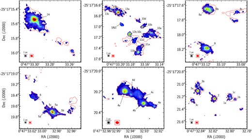
Zoom of the continuum map at 219 GHz above 5σ219 GHz (σ219 GHz = 13 |$\mu $|Jy beam−1) for the different regions containing the proto-SSCs studied in Rico-Villas et al. (2020). Overlaid, the continuum emission at 345 GHz is shown in red with contour levels at 5σ345GHz, 10σ345GHz, 25σ345GHz, and 50σ345GHz (σ345GHz = 37 |$\mu $|Jy beam−1). The different components of each SSC (in which a given SSC is fragmented) are labelled with letters. The 219 GHz beam size (0.020 arcsec × 0.019 arcsec; in black) and the 345 GHz beam size (0.028 arcsec × 0.0234 arcsec; in red) are plotted, along with a 1 pc scale, on the bottom left-hand corner for reference.
Coordinates of the peak positions at 219 GHz.
| Position | RA (J2000) | Dec (J2000) |
|---|---|---|
| 00h47m | −25°17′ | |
| 1a | 32s.8001 | 21″.220 |
| 1b | 32s.7939 | 21″.241 |
| 1c | 32s.8001 | 21″.178 |
| 2 | 32s.8186 | 21″.227 |
| 3a | 32s.8383 | 21″.101 |
| 3b | 32s.8377 | 21″.010 |
| 3c | 32s.8439 | 21″.262 |
| SN1 | 32s.8770 | 21″.360 |
| 4a | 32s.9441 | 20″.191 |
| 4b | 32s.9306 | 20″.310 |
| 4c | 32s.9327 | 20″.247 |
| 4d | 32s.9394 | 20″.226 |
| 4e | 32s.9229 | 20″.338 |
| 5a | 32s.9859 | 19″.708 |
| 5b | 32s.9787 | 19″.729 |
| 5c | 32s.9931 | 19″.624 |
| 5d | 32s.9977 | 19″.715 |
| 6 | 33s.0112 | 19″.442 |
| SN2 | 33s.0493 | 18″.833 |
| 7 | 33s.0220 | 19″.078 |
| 8a | 33s.1144 | 17″.650 |
| 8b | 33s.1108 | 17″.678 |
| 8c | 33s.0844 | 17″.692 |
| 9 | 33s.1144 | 18″.182 |
| 10a | 33s.1531 | 17″.104 |
| 10b | 33s.1634 | 17″.006 |
| 10c | 33s.1614 | 17″.146 |
| 10d | 33s.1696 | 16″.887 |
| 11a | 33s.1639 | 17″.356 |
| 11b | 33s.1696 | 17″.475 |
| 12a | 33s.1753 | 17″.272 |
| 12b | 33s.1810 | 17″.146 |
| SN3 | 33s.1934 | 16″.943 |
| 13a | 33s.1970 | 16″.733 |
| 13b | 33s.2068 | 16″.691 |
| 13c | 33s.2145 | 16″.684 |
| 14 | 33s.2955 | 15″.543 |
4 PROTO-SSC 13: A CASE STUDY
Our high spatial resolution data clearly shows a large fragmentation on the formation of massive star clusters and SSCs. To better understand the formation of SSCs and their evolution, we need to study the SSCs in their SHC phase (i.e. proto-SSC) in great detail to determine the properties of the different components detected in our maps.
In this work, we carry out a detailed study of proto-SSC 13a (i.e. SHC 13). The analysis of the other SHCs in forthcoming works will follow the procedure implemented for proto-SSC 13a. Between the two brightest sources at 219 and 345 GHz continuum emission, proto-SSC 13a was selected instead of proto-SSC 14 because the latter, despite showing brighter continuum emission at both frequencies, presents spatially asymmetric emission and complex spectral absorption features in its central region at the HC3N* spectral lines. In fact, Levy et al. (2021) recently observed P-Cygni line profiles in the CS 7−6 and H13CN 4−3 lines in the central region of SSC 14 (also in SSC 4a and SSC 5a), indicative of outflowing gas suggesting a more evolved state of evolution. Since we are interested in understanding the triggering mechanism for the formation of SSCs in galaxies and since there is no evidence for mass ejection in proto-SSC 13a, it is expected to provide a better representation of the very early stages of SSC formation.
In particular, we will address one of the main uncertainties in the previous analysis, the actual luminosities of the SHCs strongly affected by the back-warming (i.e. the greenhouse effect) and the inner kinematics unresolved by previous lower spatial resolution data. In the following sections, we present the first study of internal heating of the SHCs combining a multitransition analysis of the spatially resolved HC3N* and dust emissions with the modelling of the backwarming effect for different heating scenarios.
4.1 HC3N* emission: 2D LTE analysis of proto-SSC 13
Following Rico-Villas et al. (2020), an LTE analysis of the HC3N* emission from proto-SSC 13 was carried out with the Spectral Line Identification and Modelling (slim) module (Martín et al. 2019) within madcuba. slim is a very convenient tool for high spatial resolution spectral analysis since it allows for line identification of spectral features and its LTE analysis (including optical depth effects) directly on to spectral data. We have developed scripts to deal with the 2D determination of the LTE parameters with the slim multi line analysis including upper limits in both HC3N column densities and Tvib.
Fig. 3 shows the integrated intensity (i.e. moment 0) maps of SSC 13 from the HC3N J = 24−23 and J = 26−25 rotational transitions in the v = 0 ground state, the v7 = 1 and v6 = 1 vibrationally excited states. Among the different emitting regions that conform the proto-SSC 13 (i.e. 13a, 13b, and 13c), the only region that shows HC3N* emission is 13a, where we will focus our analysis. From the extent of the continuum emission at 219 and 345 GHz, and the emission of the v = 0 transitions, we estimate the radii of the proto-SSC 13a to be r ≈ 1.5 pc. In the moment 0 maps, in the region where the 219 GHz continuum emission peaks (the central region of SSC 13a) we observe a hole in the emission of the v = 0 lines, and also some decrease of the flux in the v7 = 1 lines. However, the moment 0 maps from the v6 = 1 lines do not show such feature. Since the v6 = 1 transitions arise from higher energies (Eup > 849 K) than the v = 0 and v7 = 1 lines (Eup < 475 K), we consider the decrease in the v = 0 and v7 = 1 to be due to absorption of the background continuum and self-absorption in the low-energy transitions instead of a true cavity at the centre of proto-SSC 13a. Also, we remind that like in galactic HCs, some uncertainty in estimating the continuum emission is present in the inner regions, where a high spectral density of absorption and emission lines typical in SHCs hamper its estimation.
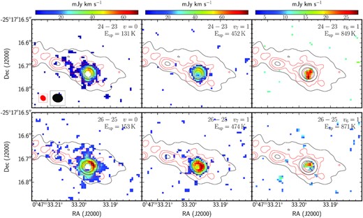
SSC 13 HC3N* moment 0 maps. The left-hand panels show the J = 24−23 (top) and the J = 26−25 (bottom) rotational transitions from the v = 0 state. The middle panels show the |$J=24-23\, l_\text{up}=1$| (top) and the |$J=26-25\, l_\text{up}=1$| (bottom) rotational transitions from the v7 = 1 vibrational state. The right-hand panels show the |$J=24-23\, l_\text{up}=-1$| (top) and the |$J=26-25\, l_\text{up}=-1$| (bottom) rotational transitions from the v6 = 1 vibrational state. Overlaid with red and black contours are the 5σ, 10σ, 50σ, and 100σ levels from the 219 GHz and 345 GHz continuum emission, respectively. Top left-hand panel shows the beam sizes of the 219 GHz (in red) and the 345 GHz (in black) continuum emission.
Besides the rotational transitions arising from the v = 0, v7 = 1, and v6 = 1 states, other HC3N* J = 24−23 and J = 26−25 rotational transitions from even higher vibrationally excited states also lie in the analysed spectral range. These vibrational excited states are v7 = 2, v5 = 1/v7 = 3, v6 = v7 = 1, v7 = 4/v5 = v7 = 1, v6 = 2, v4 = v7 = 1 and v4 = 1, v7 = 2/v5 = 20 (see table B1 in the Appendix B, available online). However, as shown in Rico-Villas et al. (2020), the proto-SSCs like proto-SSC 13a have an extremely rich chemistry and a very prominent molecular line emission from many other species, making several HC3N* transitions to be blended with transitions from other molecules. This makes that some of the weaker high-energy4 HC3N* emission lines to be blended with other species. We have been able to confirm the detection of clean or only slightly blended HC3N* emission in the v = 0 vibrational ground state and in the v7 = 1, v7 = 2, v6 = 1, v5 = 1/v7 = 3, v6 = v7 = 1, and v4 = 1 vibrationally excited states (see figures in Appendix A, available online). Transitions from the v7 = 4/v5 = v7 = 1 vibrational state are strongly blended with other lines. For higher vibrational states (v6 = 2 and v4 = v7 = 1), the expected line strength (from the CDMS5 catalogue; Müller et al. 2001, 2005) decreases by more than a |$45{{\ \rm per\ cent}}$| with respect to that of the v4 = 1 J = 26−25 transition (detected only in the most central region), and therefore are not detected. A summary of the HC3N* transitions in the observed spectral range, with their quantum numbers, energy of the upper state of the transition, frequencies, Einstein-Aul coefficients, line strengths, and if they are detected and contaminated is shown in table B1 from the Appendix.
To improve the signal-to-noise ratio for the LTE modelling, we have smoothed the spectral resolution to half the original value, down to ∼2.5 km s−1. Figures in Appendix A (available online) show the averaged spectra within rings centred on proto-SSC 13, (see Section 4.2 for the definition of these rings) with all the HC3N* transitions and other identified species also indicated for completeness. Those HC3N* lines that are blended with a line from another species but with only one transition observed for this species, are not considered for the slim LTE modelling since we cannot properly estimate the degree of blending. In case it is partially blended with another species with more than one observed transition, we also model these species and deblend its emission from that of the HC3N* emission with slim assuming the emission from the other species can be properly fitted under LTE. Also, for the central pixels within a region of ≈0.45 pc, we ignored the HC3N rotational lines from the lowest vibrational states v = 0 and v7 = 1 because they are affected by strong absorption of the continuum and self-absorption (see Fig. 3). Therefore, for the slim LTE modelling of the central region, we only considered transitions from vibrationally excited states with the highest energies, which are expected to be less affected by absorption.
Following the above procedure, we have developed madcuba scripts to carry the HC3N* LTE modelling of the HC3N* emission with slim for all pixels of the proto-SSC 13a emitting region. In order to obtain the vibrational temperature (Tvib) and the total HC3N column density (N(HC3N)), we have modelled the HC3N* J = 24−23 and J = 26−25 rotational transitions from all (excluding the v = 0 and v7 = 1 transitions in the central pixels, see above) the vibrationally excited states and the ground state simultaneously with a single temperature (i.e. the vibrational temperature Tvib). Unfortunately, the small energy difference between the J = 24−23 and the 26−25 lines and the high Tvib did not allow us to estimate the rotational temperature Trot. However, as seen in Rico-Villas et al. (2020, 2021), Costagliola & Aalto (2010), we expect Trot to be lower than Tvib. For those pixels where HC3N from the v = 0 is detected but HC3N* (from the v7 = 1) is not, we estimated an upper limit for Tvib (slim calculates these upper limits by using the 3σ upper limit to the v7 = 1 column density and the fitted column density of the v = 0 transition). The pixels where no HC3N emission is detected (i.e. no HC3N from the ground and vibrationally states) were masked with the estimated upper limits to the HC3N column density with slim (based on the rms noise of the integrated line intensity; for details, see Martín et al. 2019) assuming a Tvib ∼ 150 K (close to the median upper limit Tvib ∼ 161 K), and fixing the full-width at half-maximum (FWHM) to 30 km s−1 (close to the values where HC3N is detected) and the velocity of the local standard of rest (VLSR) to 250 km s−1 (the mean VLSR for SSC 13). We note that these N(HC3N) upper limits are conservative and probably overestimate the column density since they are obtained assuming a high excitation temperature. Fig. 4 shows the HC3N column density, vibrational temperature, VLSR, and FWHM map values derived with slim.
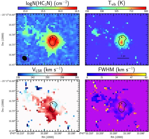
Proto-SSC 13 LTE fitted values with slim. Top left-hand panel shows the HC3N column density, top right-hand panel the vibrational temperature, bottom left the VLSR and bottom right the FWHM. The black contour indicates the region with Tvib > 500 K. To estimate upper limits to the column density we have fixed Tvib to 150 K, the VLSR to 250 km s−1 and the FWHM to 30 km s−1, and therefore these values appear as background pixels.
From Fig. 4 we can see that the region with highest HC3N column densities (≳ 1016 cm−2) is the region where we also find the highest temperatures (Tvib ≳ 400 K). There is a decrease in the column density towards the centre of proto-SSC 13a coincident with the highest temperatures. This is a spurious effect probably caused by the high opacity towards the centre. Also, while the temperature map appears symmetric, the column density map seems to be slightly elongated in the NE-SW direction along the galaxy disc, where we find a bridge of emission joining 13a with 13b, see Fig. 2. Lower left and lower right-hand panels of Fig. 4 show the velocity and the FWHM maps derived from HC3N* slim modelling. As derived in Rico-Villas et al. (2020), proto-SSC 13a has a systemic velocity of 250 km s−1. Fig. 4 clearly shows a sharp jump in the velocity along the SE-NW direction (i.e. perpendicular to NGC 253 rotation disc, with PA = 55°; Krieger et al. 2019), dividing the region with Tvib ≳ 500 K. Perpendicular to this local velocity change, i.e. the region with velocities ∼250 km s−1 along NGC 253 disc, we can see that the HC3N* FWHMs are also larger (∼35 km s−1). The possible nature and implications of the ∼21 km s−1 jump between the minimum (242 km s−1) and maximum (263 km s−1) velocities is discussed in Section 5.4.
4.2 Radial distribution of proto-SSC 13a: LTE-slim analysis
To increase the signal-to-noise ratio of the spectra, specially for the higher energy lines, and thus improve our analysis, we have averaged the spectra within rings of 0.1 pc thickness with radius increasing in 0.1 pc up to 1.5 pc, as the noise decreases with the considered number of pixels for each ring like |$1/\sqrt{N_\text{px}}$|. This is appropriate for proto-SSC 13a since it appears to be rather symmetric (e.g. see Fig. 4), with the rings centred on the pixel with the brightest continuum emission at 219 GHz (RA(J2000)=00h47m33s.1970; Dec(J2000)=−25°17′16″.733). Table 5 lists the integrated line intensities of the HC3N* transitions within the rings.
Velocity integrated line intensities of ring averaged spectra in proto-SSC 13.
| Dist. | v = 0 | v7 = 1 | v7 = 1 | v7 = 2 | v7 = 2 | v6 = 1 | v6 = 1 | v5 = 1/v7 = 3 | v6 = v7 = 1 | v4 = 1 | v6 = 2 | |
|---|---|---|---|---|---|---|---|---|---|---|---|---|
| Jup-Jlo | 26−25 | 24−23 | 26−25 | 24−23 | 26−25 | 24−23 | 26−25 | 26−25 | 26−25 | 26−25 | 24−23 | |
| lup; llo | 1; −1 | 1; −1 | 0; 0 | 0; 0 | −1; 1 | −1; 1 | 1,0; −1,0 | 2,2; −2,2 | 0; 0 | |||
| (pc) | ν (GHz) | 236.51 | 219.17 | 237.43 | 219.68 | 237.97 | 218.68 | 236.90 | 236.66 | 237.81 | 236.18 | 219.02 |
| 0.05 | ≤9.3 | |$27.2\, \pm 3.2$| | |$37.8\, \pm 1.9$| | |$28.6\, \pm 3.5$| | |$30.4\, \pm 2.2$| | |$27.9\, \pm 3.1$| | |$30.7\, \pm 2.2$| | 19.1 ± 2.1 | 19.1 ± 1.6 | 12.9 ± 1.7 | ≤9.4 | |
| 0.15 | |$21.1\, \pm 2.3$| | |$31.1\, \pm 2.2$| | |$42.2\, \pm 1.4$| | |$28.1\, \pm 2.5$| | |$30.5\, \pm 1.6$| | |$26.7\, \pm 2.2$| | |$29.9\, \pm 1.6$| | 17.8 ± 1.5 | 16.0 ± 1.1 | 10.1 ± 1.2 | ≤6.8 | |
| 0.25 | |$41.8\, \pm 1.5$| | |$37.0\, \pm 1.7$| | |$45.1\, \pm 1.0$| | |$24.4\, \pm 1.7$| | |$28.4\, \pm 1.0$| | |$23.6\, \pm 1.5$| | |$25.4\, \pm 1.1$| | 15.8 ± 1.1 | 12.9 ± 0.7 | 5.8 ± 0.7 | ≤4.9 | |
| 0.35 | |$52.6\, \pm 1.3$| | |$40.9\, \pm 1.6$| | |$42.0\, \pm 0.8$| | |$20.0\, \pm 1.4$| | |$23.6\, \pm 0.8$| | |$18.7\, \pm 1.3$| | |$17.0\, \pm 0.9$| | 10.2 ± 0.8 | 8.8 ± 0.6 | 3.5 ± 0.6 | ≤4.1 | |
| 0.45 | |$50.5\, \pm 1.3$| | |$33.7\, \pm 1.2$| | |$34.0\, \pm 0.8$| | |$17.1\, \pm 1.2$| | |$17.6\, \pm 0.8$| | |$11.9\, \pm 1.0$| | |$10.3\, \pm 0.9$| | 5.4 ± 0.7 | 4.4 ± 0.5 | 1.7 ± 0.4 | ≤2.9 | |
| 0.55 | |$41.2\, \pm 1.1$| | |$22.0\, \pm 1.2$| | |$24.4\, \pm 0.7$| | |$10.9\, \pm 1.3$| | |$11.5\, \pm 0.7$| | |$6.0\, \pm 1.1$| | |$4.9\, \pm 0.8$| | ≤1.9 | ≤1.4 | 1.0 ± 0.3 | ≤3.0 | |
| 0.65 | |$30.4\, \pm 1.0$| | |$14.4\, \pm 1.1$| | |$14.6\, \pm 0.6$| | |$6.4\, \pm 1.2$| | |$6.6\, \pm 0.7$| | ≤2.9 | |$3.9\, \pm 0.7$| | ≤1.7 | ≤1.0 | ≤0.9 | ≤2.6 | |
| 0.75 | |$21.8\, \pm 0.8$| | |$7.0\, \pm 1.0$| | |$6.6\, \pm 0.5$| | ≤3.3 | |$3.9\, \pm 0.5$| | ≤2.9 | |$2.2\, \pm 0.6$| | ≤1.4 | ≤0.9 | ≤0.8 | ≤2.4 | |
| 0.85 | |$18.3\, \pm 0.8$| | |$3.9\, \pm 0.9$| | |$2.4\, \pm 0.5$| | ≤3.3 | |$2.9\, \pm 0.6$| | ≤3.0 | ≤1.9 | ≤1.5 | ≤0.9 | ≤0.8 | ≤2.7 | |
| 0.95 | |$14.7\, \pm 0.7$| | |$2.7\, \pm 0.9$| | |$1.7\, \pm 0.5$| | ≤3.0 | |$2.0\, \pm 0.5$| | ≤2.7 | ≤1.7 | ≤1.4 | ≤0.8 | ≤0.8 | ≤2.8 | |
| 1.05 | |$10.6\, \pm 0.7$| | ≤2.4 | |$1.9\, \pm 0.5$| | – | ≤1.6 | – | ≤1.3 | – | – | – | – | |
| 1.15 | |$7.9\, \pm 0.7$| | ≤2.0 | |$1.6\, \pm 0.5$| | – | ≤1.6 | – | ≤1.3 | – | – | – | – | |
| 1.25 | |$7.3\, \pm 0.7$| | ≤2.0 | ≤1.4 | – | ≤1.5 | – | ≤1.2 | – | – | – | – | |
| 1.35 | |$7.5\, \pm 0.6$| | ≤1.5 | ≤1.1 | – | ≤1.5 | – | ≤1.0 | – | – | – | – | |
| 1.45 | |$5.8\, \pm 0.6$| | ≤1.5 | ≤1.1 | – | ≤1.2 | – | ≤1.0 | – | – | – | – |
Notes. The table lists the distance in pc to each averaged ring (i.e. (Rint + Rout)/2) with the line intensities in Jy km s−1 beam−1. The table also lists the quantum numbers and the frequency of the transition in GHz.
The v5 = 1/v7 = 3 and v6 = v7 = 1 quantum numbers refer to |$l_\text{up},\, k_\text{up}$|; |$l_\text{lo},\, k_\text{lo}$|.
The v6 = 2 24, 0−23, 0 transition is not detected in any ring, but its upper limits are included as a consistency test for the non-local radiative transfer models.
With slim, we have modelled the emission of these higher signal-to-noise ratio averaged ring spectra following the same LTE procedure described above. Figures in the Appendix A (available in the online version) show the HC3N* LTE modelled emission for the rings. We have observed that at short distances (r < 0.4 pc), HC3N* transitions from the v = 0 and v7 = 1 states show strong absorption and therefore, as described above, were not taken into account for the fit. Although for these self-absorbed, contaminated, or at noise level line profiles are simulated with slim for the derived parameters, they are not taken into account for the fitting. Therefore, some undetected lines from high vibrational states show modelled emission within noise level. Obviously, the slim models cannot reproduce all HC3N* lines simultaneously due to non-local effects that are not included. In addition, since line absorption is more important for low-energy lines than for high-energy lines, slim considers their ratio as very high Tvib. We can thus consider the slimTvib (i.e. Tdust, see Rico-Villas et al. 2020) in the innermost regions as upper limits.
Table 6 lists the distance to each ring, the number of pixels contained in the ring, and the weighted mean values (for the pixels within each ring that are not upper limits) of Tvib and N(HC3N) from the fit to the spectra of individual pixels in the image (for the pixels within each ring that are not upper limits), together with the corresponding values inferred from the averaged ring spectra. These values are plotted as a function of their distance to proto-SSC 13a centre in Fig. 5. There is a good match between both profiles, but there is a clear improvement in the error of the estimated parameters in the averaged spectra, specially in the lower signal-to-noise regions.
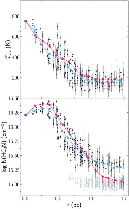
Proto-SSC 13a HC3N* vibrational temperature (Tvib) and column density (log N(HC3N)) profiles derived from the LTE model fitting with slim from Table 6. The solid black dots represent the values fitted for each individual pixel, while grey markers with arrows represent upper limits for each individual pixel. The blue markers show the weighted mean of the fitted values for the pixels (not considering the upper limits) within each ring of 0.1 pc thickness. The red markers show the fitted values for the averaged spectra of each ring.
Proto-SSC|$\, 13$|a HC3N* vibrational temperature and column density comparison between the average of fitted pixels and the fit to the average spectrum for each ring.
| Pixels mean | Averaged spectra | ||||||
|---|---|---|---|---|---|---|---|
| Dist. | # Pixels | Tvib | log N(HC3N) | Tvib | log N(HC3N) | ||
| (pc) | (K) | (cm−2) | (K) | (cm−2) | |||
| 0.05 | 1 | ≤751 | 16.21 ± 0.02 | ≤751 | 16.21 ± 0.03 | ||
| 0.15 | 8 | 656 ± 55 | 16.28 ± 0.04 | ≤611 | 16.37 ± 0.02 | ||
| 0.25 | 12 | 517 ± 66 | 16.33 ± 0.06 | ≤555 | 16.40 ± 0.02 | ||
| 0.35 | 16 | 432 ± 79 | 16.30 ± 0.11 | 505 ± 26 | 16.39 ± 0.02 | ||
| 0.45 | 20 | 404 ± 111 | 16.16 ± 0.18 | 420 ± 37 | 16.21 ± 0.02 | ||
| 0.55 | 24 | 381 ± 107 | 15.93 ± 0.20 | 384 ± 35 | 16.04 ± 0.03 | ||
| 0.65 | 28 | 306 ± 96 | 15.80 ± 0.19 | 357 ± 34 | 15.92 ± 0.02 | ||
| 0.75 | 36 | 234 ± 84 | 15.66 ± 0.15 | 280 ± 30 | 15.71 ± 0.02 | ||
| 0.85 | 32 | 202 ± 52 | 15.53 ± 0.12 | 228 ± 21 | 15.58 ± 0.02 | ||
| 0.95 | 44 | 176 ± 54 | 15.49 ± 0.13 | 214 ± 22 | 15.46 ± 0.02 | ||
| 1.05 | 56 | 179 ± 47 | 15.40 ± 0.09 | ≤186 | ≤15.23 | ||
| 1.15 | 48 | 149 ± 43 | 15.38 ± 0.08 | ≤186 | ≤15.13 | ||
| 1.25 | 48 | 149 ± 50 | 15.35 ± 0.12 | ≤186 | ≤15.11 | ||
| 1.35 | 64 | 183 ± 27 | 15.28 ± 0.12 | ≤186 | ≤15.07 | ||
| 1.45 | 60 | 167 ± 65 | 15.30 ± 0.15 | ≤186 | ≤15.05 | ||
Note. (1) Ring distance. (2) Number of pixels in each ring. (3) Weighted mean of the LTE vibrational temperature fitted for each pixel within the ring. The errors, except for ring 1 with one single pixel, are the errors of the mean. (4) Weighted mean of the LTE column density fitted for each pixel within the ring. The errors, except for the first ring with one single pixel, are the errors of the mean. (5) Fitted LTE vibrational temperature to the ring averaged spectra (i.e. the spectra obtained from averaging all the spectra from the pixels within each ring). (6) Fitted LTE column density to the ring averaged spectra.
Fig. 5 show that Tvib peaks at the central pixel (Tvib ≲ 751 K) and decreases with distance to ∼200 K at 0.85 pc. At longer distances (≳ 0.9 pc), most pixels have Tvib upper limits (i.e. no HC3N v7 = 1 line was detected) with Tvib ≲ 186 K. For the HC3N* column density, its maximum value is obtained at ∼0.25 pc. The lower column density values at smaller distances are probably an artefact produced by the strong absorption towards the central region, which still affects even the strength of the v6 = 1 and v7 = 2 lines. We note that the fitted averaged spectra values start to differ from the pixel mean values at distances ≳ 1.0 pc as a result of averaging all pixels (with and without HC3N* column density upper limits in each individual pixel).
4.3 Radial distribution of proto-SSC 13a: Non-local analysis
As seen in Rico-Villas et al. (2020), LTE can be assumed for the excitation of the HC3N* emission when there is a strong IR radiation field and a high dust optical depth in the mid-IR. This is because HC3N molecules will be immersed in a local radiation field described by a blackbody at the dust temperature (i.e. Tvib ∼ Tdust) and their ro-vibrational transitions (excited by ∼11−45 |$\mu $|m radiation) will be thermalized independently from their Einstein-Aul coefficients and H2 density. However, the large column densities that in principle validate LTE excitation, make non-local radiative transfer effects very important: the large amounts of gas and dust increase the probabilities for a photon emitted in some region at that local Tdust to be absorbed in another region at |$T^\prime _\text{dust}$|, even more than once, before reaching the observer. In addition, in the case of density and temperature gradients within the SHCs, the high line opacities will make every line to trace different excitation temperatures. We have then carried non-local radiative transfer models of the HC3N* emission assuming LTE excitation for all states. We have assumed LTE excitation since, as already mentioned, all HC3N* lines are expected to be thermalized at Tdust. Also, the Aul coefficients from many of the ro-vibrational bands are not available, preventing to carry a full non-LTE excitation modelling for all the observed lines.
The radiative transfer models are based on the radiative transfer code developed by González-Alfonso & Cernicharo (1997, 1999) and González-Alfonso & Sakamoto (2019), with the inclusion of the v5 = 1/v7 = 3, v6 = v7 = 1, v4 = 1, and v6 = 2 vibrationally excited states up to high J values (J = 50) and assuming thermalization (i.e. local LTE excitation). These models aim at reproducing the spatial profile of the emission from the detected, unblended, and uncontaminated HC3N* transitions listed in Table 5. These transitions cover a wide range of energies, from 142 K to 1579 K. The v6 = 2 (24, 0−23, 0) transition is not detected and is included in the models as a control to the HC3N column density and vibrational temperature. Emission lines are self-consistently fitted together with the radial profiles of the continuum emission at 235 and 345 GHz obtained from the ring spectra (top left-hand panel of Fig. 6).
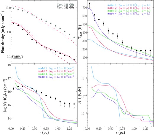
Observed and modelled continuum emission and parameters used each model (Model 1 in blue, Model 2 in red, Model 3 in green, and Model 4 in purple) profiles. Upper left-hand panel shows the rings continuum emission at 235 GHz with a resolution of 0.022 arcsec × 0.020 arcsec (black filled circles) and at 345 GHz at a resolution of 0.028 arcsec × 0.034 arcsec (grey filled circles). The dashed red lines show the continuum emission from Model 2 (q = 1.5) resulting from the Tdust profile for both frequencies, while the red solid line shows the continuum emission at 235 GHz resulting from the modelling after varying Xd to account for both the free–free emission in the innermost region and the excess of continuum emission in the outermost region. Upper right-hand and lower left-hand panels show the dust temperature (∼Tvib) and column density profiles obtained from the slim LTE model (black filled circles) for the averaged ring spectra and the solid coloured lines indicates the profiles of each non-local model. Lower right-hand panel solid coloured lines show the HC3N abundance profiles for each model. Half of the beam FWHM (i.e. 0.011 arcsec) is shown on the upper right-hand panel.
Regarding the thermal structure of the SHC, we have used different density and Tdust radial profiles derived following González-Alfonso & Sakamoto (2019), which take into account the greenhouse effect expected for the very large column densities (|$N_{\text{H}_2}\gt 10^{24}$|) derived in Rico-Villas et al. (2020). The Tdust profiles are obtained in a self-consistent way considering the heating and cooling of dust grains in a spherical cloud with a given density profile. Input model parameters are the luminosity surface density ΣIR = LIR/(πR2), the H2 column density N(H2), the density profile (parametrized with q as |$n_{\text{H}_2}\propto r^{-q}$|) and the absorption coefficient of dust as a function of wavelength κabs(λ). The derived temperature profiles also depend on the nature of the heating source (point source and centrally peaked). For the case of SSCs, we use the centrally peaked starburst profiles from González-Alfonso & Sakamoto (2019), which consider the deposition of energy due to star formation to be distributed across the cloud and proportional to the shell density and mass, in contrast with a single point source heating, expected for the AGN models (González-Alfonso & Sakamoto 2019). The models are then described by the source radius rout, a total LIR, a total gas H2 column density |$N_{\text{H}_2}$|, and the density profile power-law index q. These parameters define consistently the Tdust profile for the type of heating (star formation or AGN) used in our radiative transfer predictions. Hence, the only free-parameters are the HC3N abundance relative to H2 (|$X_{\text{HC}_3\text{N}}$|), which we vary for each shell to fit the observed spatial profiles, and Xd which reflects the amount of dust relative to gas (by mass).
We find that the ratio between the 235 and 345 GHz continuum emission increases for r < 0.85 pc (once corrected for the different beams), indicating the presence of free–free emission. To account for this free–free emission observed at the center we use the Xd parameter, which is boosted in the central region to mimic such free–free emission. For r < 0.85 pc, the extra continuum added accounts for a total of 1.89 mJy at 235 GHz, very similar to the estimated non-dust contribution (|$S_{219_\text{n-dust}}=1.99$| mJy) obtained by assuming a spectral index expected for optically thin dust emission of α345 − 219 ∼ 3.5. In the outer region (i.e. r ≳ 0.85 pc), Xd is also adjusted to fit the observed 235 GHz emission, which translates into a higher column and mass of gas and dust relative to the power-law density profile. This is because no single value of q can describe the whole spatial profile of the observed continuum emission. Accordingly, we consider the excess of dust added up to 0.85 pc as free–free emission and from 0.85 pc to 1.5 pc as an increase in mass that deviates from the |$n_{\text{H}_2}\propto r^{-q}$| assumed profile.
From the continuum emission6 at 219 GHz (0.5 pc × 0.5 pc) and at 345 GHz (0.8 pc × 0.8 pc) and the extent of the HC3N v = 0 emission (see Figs 3 and 4), we modelled proto-SSC 13a up to a radius of 1.5 pc considering several density and temperature profiles.
4.3.1 Non-local modelling results
Figs 6 and 7 show the results for four representative models with star formation heating that best reproduce the continuum and the HC3N* line emission. The models have an H2 column density of ∼1025 cm−2 with two different density profiles (q = 1 and q = 1.5, modified as indicated above), and cover two different IR luminosities (LIR) of 9.2 × 10⁷ L⊙ and 3.9 × 10⁸ L⊙. These luminosities are close to the protostar luminosity of 108 L⊙ derived in Rico-Villas et al. (2020) for proto-SSC 13. A summary of the parameters of the most representative models, labelled 1 to 4, is shown in Table 7. Since we have corrected the model masses to fit the 235 GHz continuum emission in the outer regions (i.e. 0.85−1.5 pc), models with the same luminosity but different q index have similar final gas masses.
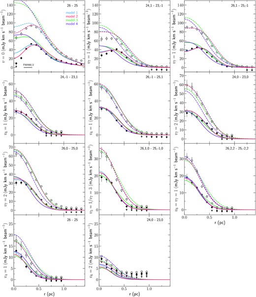
Observed and modelled HC3N* line emission spatial profiles of the transitions listed in Table 5. The black filled and open circles show the integrated line intensity of the averaged ring spectra at 0.022 arcsec × 0.020 arcsec and 0.028 arcsec × 0.034 arcsec resolution, respectively, for each HC3N* transition (quantum number of the transition are indicated on the upper right corner of each panel). Coloured lines show the modelled emission for each model (Model 1 in blue, Model 2 in red, Model 3 in green and Model 4 in purple) at a resolution of 0.022 arcsec × 0.020 arcsec (solid lines) and 0.028 arcsec × 0.034 arcsec (dashed lines). Half of the beam FWHM is shown on the first panel.
Parameters of the non-local radiative transfer models for the case of heating due to distributed star formation.
| Model | q | LIR | ΣIR | |$M_{\text{H}_2}$| | |$L_\text{IR}/M_{\text{H}_2}$| | re | |$N_{\text{H}_2}$| | |$N_{\text{HC}_3\text{N}}$| | |$\chi ^2_\text{lines}$| | Type |
|---|---|---|---|---|---|---|---|---|---|---|
| (pc) | (L⊙) | (L⊙ pc−2) | (M⊙) | (L⊙/M⊙) | (pc) | (cm−2) | (cm−2) | |||
| 1 | 1.0 | 9.4 × 10⁷ | 1.3 × 10⁷ | 9.4 × 10⁵ | 100 | 0.8 | 1.0 × 1025 | 1.1 × 10¹⁸ | 5.1 | Dist. |
| 2 | 1.5 | 9.4 × 10⁷ | 1.3 × 10⁷ | 9.5 × 10⁵ | 99 | 0.4 | 1.2 × 1025 | 3.1 × 10¹⁷ | 4.5 | Dist. |
| 3 | 1.0 | 3.9 × 10⁸ | 5.5 × 10⁷ | 6.0 × 10⁵ | 656 | 0.8 | 9.2 × 1024 | 1.3 × 10¹⁷ | 16.6 | Dist. |
| 4 | 1.5 | 3.9 × 10⁸ | 5.5 × 10⁷ | 6.1 × 10⁵ | 638 | 0.4 | 1.0 × 1025 | 9.7 × 10¹⁶ | 11.0 | Dist. |
| 5 | 1.5 | 9.8 × 10⁷ | 1.4 × 10⁷ | 7.8 × 10⁵ | 126 | − | 1.1 × 1025 | 1.3 × 10¹⁷ | 7.2 | Central |
| 6 | 1.0 | 9.8 × 10⁷ | 1.4 × 10⁷ | 9.0 × 10⁵ | 109 | − | 1.0 × 1025 | 1.3 × 10¹⁷ | 10.9 | Central |
| 7 | 1.0 | 9.8 × 10⁷ | 1.4 × 10⁷ | 8.4 × 10⁵ | 117 | − | 6.9 × 1024 | 1.9 × 10¹⁷ | 6.0 | Central |
Notes. All models have r = 1.5 pc. q is the power-law index assumed for the density profile. LIR and ΣIR are the luminosity and the luminosity surface density. |$M_{\text{H}_2}$| is the model total mass and |$L_\text{IR}/M_{\text{H}_2}$| the luminosity per unit of mass. re is the radius containing half of the star formation for distributed star formation models, which is |$\propto n_{\text{H}_2}M_{\text{H}_2}$| for each shell (see González-Alfonso & Sakamoto 2019). For central star formation models, all the star formation is contained inside r < 0.05 pc. |$N_{\text{H}_2}$| and |$N_{\text{HC}_3\text{N}}$| are to the total H2 and HC3N column densities. |$\chi ^2_\text{lines}$| is the average of the |$\chi ^2_\text{line}=\sum \limits _{i} \frac{(o_i-m_i)^2}{n \delta _{o_i}^2}$| for each line, where oi and mi are the observed and modelled line intensities, n the number of points taken into account, and |$\delta _{o_i}$| is the observed error. Type refers to distributed or central star formation models.
Fig. 6 shows, in the upper left-hand panel, the observed 235 GHz continuum emission at a 0.022 arcsec × 0.020 arcsec resolution (filled black circles) and the 345 GHz continuum emission at a 0.028 arcsec × 0.034 arcsec resolution (filled grey circles). The dashed lines represent the predicted continuum emission profiles of Model 2 (q = 1.5) at 235 and 345 GHz for the corresponding Tdust profiles from González-Alfonso & Sakamoto (2019). The solid line show the continuum emission at 235 GHz derived from our modelling after varying Xd. Fig. 6 also compares the modelled Tdust spatial profile considering the greenhouse effect for the different density profiles and luminosities. It also shows the HC3N column density profiles (solid lines) with the values derived from slim in Section 4.2 (filled black circles) and the HC3N abundance relative to H2 (X(HC3N)). Despite having similar H2 column densities and/or LIR, the difference in the density power-law index q (q = 1.0 or q = 1.5 for |$n_{\text{H}_2}\propto r^{-q}$|), translates into different H2 densities and Tdust within a given shell, resulting in the different |$N_{\text{HC}_3\text{N}}$| and |$X_{\text{HC}_3\text{N}}$| profiles plotted in Fig. 6. All models reproduce well the observed 235 GHz continuum emission, which, as expected, clearly shows that the models constrained only by dust emission are degenerated. Further constraints to the models are provided by considering the emission from the multiple detected HC3N* lines as a function of the radius.
4.3.2 Breaking the model degeneracy using HC3N* emission
Fig. 7 shows the observed HC3N* emission radial profiles at a resolution of 0.022 arcsec × 0.020 arcsec (filled black circles) and at a resolution of 0.028 arcsec × 0.034 arcsec (open circles) for the HC3N* transitions listed in Table 5. The modelled HC3N* radial profiles are also plotted at both resolutions with solid and dashed, respectively, coloured lines for each model. Fig. 7 shows that most lines from high vibrational excited states (high-energy lines) are well reproduced by the four models. Considering only these high-v lines, there is still a degeneracy between the considered models. Lowering Tdust (as in models 1 and 2, Fig. 6) decreases the emission of the high-energy transitions, which requires to significantly increase the HC3N abundance in the hotter inner shells to reproduce the high-energy observed emission. Increasing |$n_{\text{H}_2}$| rises the HC3N column density and therefore the HC3N emission, which can be decreased by lowering its HC3N abundance. However, we can favour one model over another by taking into account also the low-v lines (including the v = 0) and the physical constraints of the assumed model parameters.
4.3.3 Model discrimination
As already mentioned, the models are somewhat degenerated if only the continuum emission and/or very high-energy HC3N* lines are considered, but one can break the degeneration by taking into account also the HC3N lines arising from the v = 0 and v7 = 1 states.
We propose to consider simultaneously both the high-energy and the low-energy transitions ratios to increase the dynamic range in energy. Such large energy range can be used thanks to the large number of HC3N* transitions in the observed frequency range. We show in Fig. 8 the ratio between the v7 = 1 (24, 1 − 23, −1) and the v6 = 1 (24, -1 − 23, 1) (i.e. [v7 = 1]/[v6 = 1]) as representative of the low-energy transitions and the ratio between the v6 = 1 (24, -1 − 23, 1) and the v6 = v7 = 1 (26, 2, 2 − 25, −2, 2) (i.e. [v6 = 1]/[v6 = v7 = 1]) as representative of the high-energy transitions. We can see that Model 3 and Model 4 fail to reproduce both line ratio profiles simultaneously. In the innermost region the [v6 = 1]/[v6 = v7 = 1] is close to the observed ratio but the [v7 = 1]/[v6 = 1] ratio is far from being reproduced; the opposite effect is found for the [v7 = 1]/[v6 = 1] ratio. On the other hand, Model 1 and Model 2 reproduce both ratios at the same time for all radii, with Model 2 predicting values closer to the observed ratios. Clearly, Models 3 and 4 grossly overestimate the emission of the low-energy v = 0 and v7 = 1 from the innermost rings, while Models 1 and 2 agree much better with observations.
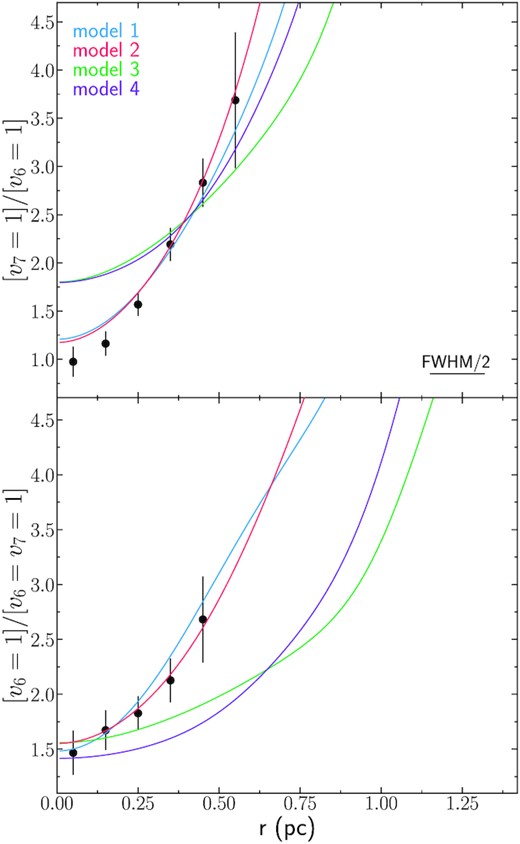
Observed and modelled HC3N* line ratios radial profiles. Left-hand panel shows the ratio between the v7 = 1 (24, 1 − 23, −1) and the v6 = 1 (24, −1 − 23, 1) transitions. Right-hand panel shows the ratio between the v6 = 1 (24, −1 − 23, 1) and the v6 = v7 = 1 (26, 2, 2 − 25, −2, 2) transitions.
From the line integrated intensity radial profiles and from the [v7 = 1]/[v6 = 1] and [v6 = 1]/[v6 = v7 = 1] line ratios profiles (Figs 7 and 8), Model 1 and Model 2 are the best in reproducing all spatial profiles (they have the lowest |$\chi ^2_\text{lines}$| values, see Table 7). These include the absorption features in the inner rings from the low-energy ground state v = 0 and v7 = 1 transitions, and both line ratios. Between these two models, Model 2 is favoured against Model 1 because Model 2 reproduces better the [v7 = 1]/[v6 = 1] and [v6 = 1]/[v6 = v7 = 1] line ratios. Also, for Model 1, the v = 0 line is not reproduced. Even Model 2, while showing a stronger decrease in the v = 0 flux towards the centre, still cannot fully reproduce it, suggesting that the HC3N column density towards the innermost rings is somewhat higher than in the model. Moreover, Model 1 requires a rather ‘strange’ HC3N abundance profile (with very high abundances towards the centre, see Fig. 6) in order to reproduce the distributions of the high-energy lines.
In summary, assuming spherical symmetry with a temperature and density radial profiles obtained in a consistent way considering the heating from the greenhouse effect due to the large optical depths in the IR and distributed star formation heating, Model 2 is able to reproduce the radial distribution of the continuum and the HC3N* emission.
5 DISCUSSION
5.1 Dust temperature profiles derived from local and non-local radiative transfer analysis
If we compare the Tdust and the N(HC3N) profiles derived from Model 2, which take into account non-local radiative transfer effects, with those derived from the slim LTE analysis, we can see very significant differences in both profiles (see Fig. 6). The differences in the dust temperature (overall higher Tdust values for the slim model) arise from the fact that the slim LTE model does not include non-local radiative transfer effects along the line of sight, which are crucial for the large column densities, H2 density, and dust temperature profiles expected in the very early phases of the SSCs formation. These effects give rise to the absorption features in the inner regions for the lines of the low v = 0 and v7 = 1 vibrational states, which decrease their intensities in relation to higher-v transitions, indicating that lines from different vibrational states arise from different regions and thus sample different physical conditions along the line of sight. When these transitions are not taken into account to avoid this effect, as considered for the slim model inner regions, the covered energy range is reduced and the slim fit tends to rise Tdust as the absorption also affects the v7 = 2 and v6 = 1, although to a lesser extent than for the v = 0 and v7 = 1. Even at large radii, the LTE dust temperature is overestimated. This is due to the combination of different optical depths in the v = 0 and the v7 = 1 lines and the Tdust radial gradient, making both lines to trace the region where they become optically thick and therefore tracing different Tdust within the proto-SSC. Since the v = 0 lines are optically thick at larger radii where the v7 = 1 lines are optically thin, the Tdust traced by the v = 0 lines will be smaller than that from the v7 = 1 lines. This effect will also appear for any pair of lines from different vibrationally excited levels. Also, since the rings width is smaller (0.1 pc) than half of the beam FWHM (0.17 pc), which is the true resolution power of the observations, each ring has also a contribution from the adjacent rings in the sky plane, however we expect it to affect to a lesser extent the differences in the Tdusts profile than the contribution from other rings along the line of sight. Regarding the HC3N column density, its profile is similar at small radii to that of the non-local models, but at longer radii (>0.7 pc) they start to differ significantly. This is partially due to subthermal excitation (difference between Trot and Tvib) found in Costagliola & Aalto (2010) and Rico-Villas et al. (2021), which tends to overestimate the LTE HC3N column densities when considering Tvib, instead of Trot, for the calculation in slim. Observations of less abundant isotopologues will help us to alleviate the optical depth problems in the LTE analysis. Unfortunately, the isotopologues lines are weaker and the potential lines to be detected in extragalactic sources will be limited to the lines arising from the lowest vibrational levels.
5.2 Central versus distributed star formation
The models described above assume that the star formation spatial profile is proportional to the gas density and mass, injecting energy from stars at different radii. The energy deposition per unit of time and volume is proportional to the SFR per unit of volume (see González-Alfonso & Sakamoto 2019, for details). This is reflected in the different Tdust profiles for a given column density and power-law index q. Consequently, a q = 1.0 index represents a more scattered star formation than a q = 1.5 index, as illustrated by re, the radius that contains half of the star formation (i.e. luminosity). Models with q = 1.0 have a more extended re of ∼0.8 pc and models with q = 1.5 a smaller re ∼ 0.4 pc. The selected model, i.e. Model 2, has a q = 1.5 (re ∼ 0.4 pc), indicating that a higher concentration of star formation (or the most massive stars) is located at the centre of proto-SSC 13a, although a fraction of the star formation also takes place at larger radii.
To test the assumption of distributed star formation in the proto-SSC 13a, we have also modelled the HC3N* and continuum emission assuming that the star formation only takes place in the very central region (∼0.05 pc, i.e. central star formation). To do so, we have used the ‘AGN’ model profiles for Tdust from González-Alfonso & Sakamoto (2019). Fig. 9 compares the distributed star formation Model 2 with three central star formation models (Models 5, 6, and 7). The three models have the same luminosity as Model 2 (LIR = 9.2 × 10⁷ L⊙), and Models 5 and 6 also the same column density (|$N_{\text{H}_2}=10^{25}$| cm−2), but Model 7 has a lower column density (|$N_{\text{H}_2}=5.6\times 10^{24}$| cm−2). For the same luminosity and column density as the models with distributed star formation from Section 4.3, the central star formation models have much steeper Tdust profiles. Due to the small size of the region forming stars of ∼0.05 pc located in the centre, the greenhouse effect makes radiation to escape more difficult than if star formation were distributed all over the source for the same dust column density. In the outermost regions, however, the central and distributed star formation models have similar dust temperatures.

Central star formation models suffer similar problems as Models 3 and 4: the high temperature in the central region boosts too much the high-energy transitions, requiring lower abundances than Model 2. To compensate this, we lower the column density to 5.6 × 1024 cm−2 in Model 7, which allows us to maintain similar abundances as in Model 2. However, lowering the column densities reduces the absorption effect of Model 2, so that Models 5, 6, and 7 strongly overestimate the emission of the low-energy lines (mostly the v = 0). Fig. 10 shows the comparison of the low-energy [v7 = 1]/[v6 = 1] line ratio and the high-energy [v6 = 1]/[v6 = v7 = 1] line ratio between these models. Model 7, despite reproducing well the [v6 = 1]/[v6 = v7 = 1] ratio, fails to reproduce the low-energy [v7 = 1]/[v6 = 1] as it underestimates the v6 = 1 (24, −1 − 23, 1) emission at r > 0.1 pc and with its lower column density is unable to reproduce the absorption observed in the v7 = 1 and v = 0 line profiles.
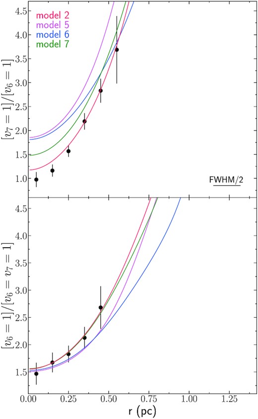
Same as Fig. 8 but with Model 2 (in red), Model 5 (in magenta), Model 6 (in dark blue), and Model 7 (in dark green).
All the temperature profiles from our modelling show that massive star formation is concentrated in the central region of proto-SSC 13a. However, we have discarded Model 7 (the best model with only star formation at the centre), since it does not reproduce simultaneously the low-energy line profiles and the [v6 = 1]/[v6 = v7 = 1] line ratio. For models with distributed star formation, Model 2 best matches the observations and both line ratios. Therefore, our modelling indicates that the most massive star formation is taking place in the central region of proto-SSC 13a (with re ∼ 0.4 pc), but star formation is distributed over a more extended region (|$\sim 80{{\ \rm per\ cent}}$| of the star formation takes place inside r = 0.9 pc).
5.3 Star formation scenarios
A centrally peaked but distributed star formation would be in accordance with the competitive accretion scenario, where most massive stars are being formed at the centre of cluster potential well and less massive stars at the outskirts (e.g. Bonnell et al. 1997, 2001; Murray & Chang 2012). Also, this would mean that mass segregation (i.e. the most massive stars in the centre of a star cluster) observed in more evolved SSCs (Bonnell et al. 2001; Bonnell, Larson & Zinnecker 2007) is already set in place at the early ages of proto-SSC 13a (tage ∼ 4 × 10⁴ yr, see Rico-Villas et al. 2020) as the competitive accretion naturally predicts. Furthermore, it has also been suggested that primordial mass segregation is present in the star clusters of the Milky Way (less massive than SSCs; e.g. McMillan, Vesperini & Portegies Zwart 2007; Pavlík, Kroupa & Šubr 2019) or in the much older (and comparable in mass to SSCs) globular clusters of the Milky Way with typical half-light radii of ∼3 pc (e.g. Haghi et al. 2014).
5.4 The proto-SSC 13a velocity structure: cloud–cloud induced star formation
From the 2D analysis of the HC3N* emission in Section 4.1 we have seen that there is a velocity structure in proto-SSC 13a that can provide information on the triggering process of the formation of SSCs. We find a separation of ∼21 km s−1 between the minimum (242 km s−1) and maximum (263 km s−1) velocities in proto-SSC 13a. Here we briefly discuss three possible origins: rotation, outflow, or cloud–cloud collision.
We can discard that the cloud is rotating. Fig. 4 shows that the local velocity change occurs in the south-east-north-west (SE-NW) direction, just perpendicular to the rotation of the galaxy disc in the northeast-southwest (NE-SW) direction. Such rotation pattern would be hard to explain in the context of the NGC 253 disc kinematics and the conservation of angular momentum. Furthermore, in Fig. 4 we can see that the region with larger velocities (250–263 km s−1) is extended towards the north-east and also surrounds the region with lower velocities (243−250 km s−1) on the west, difficult to match with a rotation pattern. Fig. 11 shows the velocity profile through the local velocity change (i.e. the SE-NW direction). It can be seen that there are two differentiated regions with different velocities: a larger cloud with velocities going from ∼263−250 km s−1 and a smaller cloud with ∼250−242 km s−1.
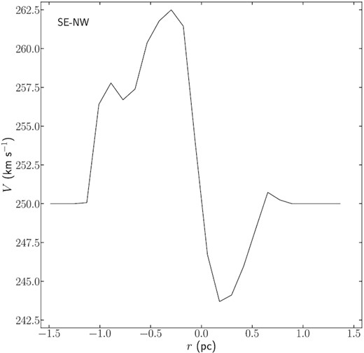
Proto-SSC 13a velocity profiles derived from the slim fitted values in the south-east-north-west direction (i.e. perpendicular to the galaxy rotation plane) in the left-hand panel and in the northeast-southwest direction (i.e. parallel to the galaxy rotation plane) in the right panel.
If the local velocity change is caused by outflowing gas, we should see the characteristic P-Cygni profiles in some of the observed transitions, or at least line wings in the spectra of the lowest energy lines. However, we do not observe such features despite the large column densities present in proto-SSC 13a. Also, as indicated by Levy et al. (2021), some vibrationally excited emission lines are coincident with the blueshifted absorption (in our case the v5 = 1/v7 = 3 line is coincident with the v = 0 line) could help us to conceal the P-Cygni profiles. Because of this, Levy et al. (2021) do not observe clear P-Cygni profiles for SSC 13a in their study of the CS 7−6 and H13CN 4−3 transitions, as they do for SSCs 4a, 5a, and 14.
Since the outflow cannot be completely ruled out, we estimate some of its properties. We consider that the systemic velocity of the SSC is 250 km s−1 and the gas is outflowing with a projected velocity of 10−15 km s−1. Note that the outflow terminal velocity would be larger since the outflow might not be along the line of sight. Assuming a 45° inclination, the terminal velocity would be about 20 km s−1. We can derive the mass of the outflowing small cloud with velocities <250 km s−1 from the total gas mass (|$M_{\text{H}_2}=9.5\times 10^5$| M⊙) and density profile (|$n_{\text{H}_2}\propto r^{-1.5}$|) obtained in Section 4.3.3 for Model 2. The outflowing mass for the blueshifted cloud with <250 km s−1 would be |$M_{\text{out,H}_2}\sim 7\times 10^4$| M⊙. Unfortunately, the estimate of the mass of the redshifted cloud is more complicated, since it merges with the ambient gas which is not expected to be participating in the outflow. We thus guess that it has a similar mass that the blueshifted gas. We can also estimate the dynamical age of the outflow by considering the distance of the outflowing cloud to its origin and the terminal velocity (δv = 21 km s−1). For a distance of ∼0.2 pc (i.e. the position of the blueshifted cloud from the expected origin) we obtain a dynamical age tdyn ∼ 104 yr. With these parameters we estimate its momentum flux by |$\dot{P}_\text{out}=\dot{M}_\text{out}\delta v=9.3\times 10^{32}$| g cm s−2, where |$\dot{M}_\text{out}=M_{\text{out,H}_2}/t_\text{dyn}$|. If we consider that the outflow is only driven by radiation, |$\dot{P}_\text{out}$| should be compatible with ∼LIR/c = 1.3 × 1031 g cm s−2 (see Murray, Quataert & Thompson 2005), which is not the case. The latter and the lack of observed P-Cygni profiles, are in agreement with the idea that proto-SSC 13a is very young and where very likely the mechanical feedback from stars is not yet affecting significantly its gas content.
We now consider the possibility of a cloud–cloud collision in which the gas with velocities ∼242−250 km s−1 would be in a cloud of 7 × 10⁴ M⊙ which is driving into a larger cloud of 8.8 × 10⁵ M⊙ with velocities ∼250−263 km s−1. The velocity of the small colliding cloud is also consistent with the non-disc component identified in the study of NGC 253 kinematics from CO emission by Krieger et al. (2019). This scenario also fits within the observed velocity structure shown in Fig. 4, with the smaller cloud being surrounded by the large cloud which still maintains its velocities, and is similar to what is expected in the early stages of a cloud–cloud collision (e.g. Habe & Ohta 1992; Takahira, Tasker & Habe 2014; Haworth et al. 2015). At the collision front, a dense layer of material is developed as the small cloud advances through the large cloud, inducing the formation of gravitationally unstable cores that lead to massive star formation (Inoue & Fukui 2013). Such external triggering of massive star formation has been invoked for the formation of several young massive clusters (YMCs) of the Milky Way and of the Large Magallanic Cloud (e.g. Furukawa et al. 2009; Ohama et al. 2010; Fukui et al. 2016, 2018; Fujita et al. 2021; Tsuge et al. 2021).
The compressed interface layer between the two clouds is usually translated into a region with intermediate velocities connecting the two clouds (i.e. a bridge feature) separated in velocity (but not spatially) in a position–velocity diagram (hereafter p-v diagram) like those shown in Fig. 12. In the HC3N column density p-v diagram (Fig. 12 left-hand panel) we can see the bridge feature with intermediate velocities connecting the two colliding clouds separated in velocities. However, in the p-v diagram of the vibrational temperature (Fig. 12 right-hand panel), the bridge feature is less clear and no clear pattern of the highest temperatures, which one would expect to be located in the bridge feature, is observed. Still, the overall velocity structure seems to favour the cloud–cloud collision scenario rather than the outflow.
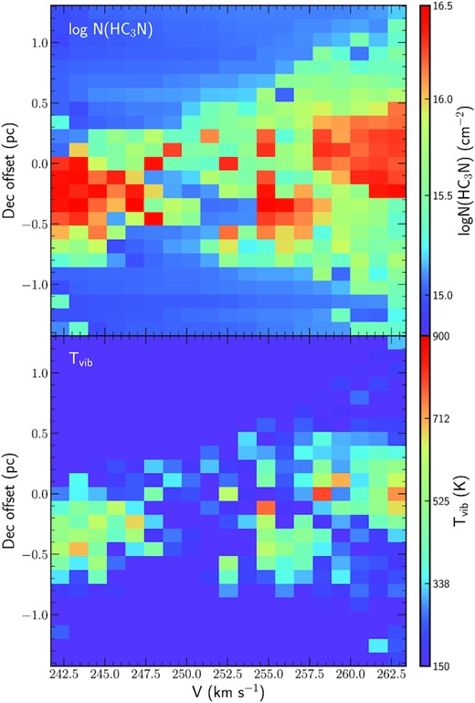
Proto-SSC 13a position velocity diagrams of the HC3N column density (top panel) and the vibrational temperature (bottom panel) derived with slim.
5.5 Derived properties for Proto-SSC 13a
The derived radius of 1.5 pc for proto-SSC 13a is close to the smallest observed SSCs, which have typical radius between 1 and 5 pc. From Model 2, we obtain for proto-SSC 13a a luminosity of LIR = 9.4 × 10⁷ L⊙, a luminosity surface density of 1.3 × 10⁷ L⊙ pc−2, and a molecular gas mass of |$M_{\text{H}_2} = 9.5\times 10^5$| M⊙ (see Table 7).
5.5.1 SSC formation through rapid collapse
From the total gas mass obtained for proto-SSC 13a we can derive its virial parameter |$\alpha =5\sigma ^2 R/GM_{\text{H}_2}$|, where σ is the velocity dispersion. From the mean of all the fitted FWHMs for each pixel in Section 4.1 (∼25 km s−1) we obtain a mean |$\bar{\sigma }\sim 11$| km s−1. Using this |$\bar{\sigma }$|, the virial parameter is α ≈ 0.21, well below the value of 2 to consider the cloud to be bounded and thus being supercritical. If we take into account the derived density profile in the innermost region (|$n_{\text{H}_2}\propto r^{-1.5}$|), α would be even smaller (Kauffmann, Pillai & Goldsmith 2013). In this supercritical state (α ≪ 2), proto-SSC 13a would be unstable and indicates a rapid collapse. Such a low virial parameter is typically found in high-mass star forming clumps and cores (see Kauffmann et al. 2013, for a review on regions with supercritical virial parameters).
5.5.2 Short time-scales and high SFE
Since proto-SSC 13a is collapsing, we can estimate its free-fall time from |$t_\text{ff}=\sqrt{3\pi /\left(32\text{G}\bar{\rho }\right)}$|, where |$\bar{\rho }$| indicates the mean gas density. For proto-SSC 13a, |$\bar{\rho }=4.5\times 10^{-18}$| g cm−3, which gives a free-fall time tff = 3 × 10⁴ yr, very similar to its estimated age (tage ∼ 4 × 10⁴ yr) in Rico-Villas et al. (2020). The small α and a tff ∼ tage ∼ 104 yr indicate that proto-SSC 13a has just started to form stars and that it is doing so very rapidly. This would be in accordance with the lack of detection of outflow signatures, which would not have had enough time to develop and/or alter the gas content.
The high SFR (3 − 5 M⊙ yr−1) derived for the individual proto-SSC 13a (and also for the remaining SSCs seen in Rico-Villas et al. 2020) contrasts with the low SFR if derived from the IR luminosity following the relation given by Kennicutt (1998) (and other similar relations) of SFR|$=4.5\times 10^{-44}L_\text{IR}(\text{erg}\, \text{s}^{-1})\approx 0.01$| M⊙ yr−1. This is because these relations are meant for entire galaxies and therefore, in order to calibrate their SFR–LIR relation, they assume continuous star formation over (10−100) × 106 yr. These large time-scales are not comparable to the young ages of the SSCs forming stars in NGC 253 much shorter ((1−10) × 104 yr) time-scales. Hence, the SFRs we derive in Rico-Villas et al. (2020) and in this paper can be understood as an instantaneous SFR. In fact, the factor ∼300 between the SFR derived in this paper and that from the relation given by Kennicutt (1998), is similar to the factor between the different time-scales considered of 3 × 10⁴ yr and 107 yr.
5.5.3 Triggering the SSC formation
5.6 Comparison to other buried star forming regions
Due to the deeply buried nature of proto-SSC 13a in the SHC phase, we can compare the results obtained for proto-SSC 13a with similar embedded sources. On the lower luminosity end, we can compare the SHC phase in proto-SSC 13a to the Milky Way HCs. In fact, the SHC phase observed in proto-SSC 13a seems to be a scaled-up version of Milky Way HCs. HCs, with luminosities ≲ 107 L⊙, are heated by a few massive protostars in a small cluster. In order to compare to proto-SSC 13a, we selected the HCs sample from Rolffs et al. (2011) (see Table 8) since they derive their masses in a similar fashion as in our radiative transfer modelling (Section 4.3), taking into account the high opacity at the centre of HCs and modelling the continuum emission accordingly (i.e. including the trapping of radiation or greenhouse effect) together with the emission from vibrationally excited HCN. We use the IRAS luminosities and the FWHMs from the ATLASGAL survey at 870 |$\mu $|m (345 GHz) listed in Rolffs et al. (2011) Table 1 (see references therein). Additionally, for SgrB2(M) and SgrB2(N) HCs, we also use the values derived by Etxaluze et al. (2013) from Herschel observations. On the higher luminosity end, we have the highly obscured nuclear regions of (U)LIRGs. These buried galactic nuclei (hereafter BGNs; also known as CONs; Falstad et al. 2021) have large column densities (|$N_{\text{H}_2}\gt 10^{24}$| cm−2) that span through the compact nuclear region (≲ 100 pc) with very high luminosities (LIR ≳ 1011 L⊙) powered by a starburst and/or an AGN. The BGNs parameters listed in Table 8 are taken from González-Alfonso & Sakamoto (2019) and the masses from González-Alfonso et al. (2015) (see also references therein). For most sources, different values of R and LIR are given, reflecting the uncertainty in their estimation.
| HC | D | R | LIR | ΣIR | |$M_{\text{H}_2}$| | |$L_\text{IR}/M_{\text{H}_2}$| |
|---|---|---|---|---|---|---|
| Source | (kpc) | (pc) | (105 L⊙) | (105 L⊙ pc−2) | (103 M⊙) | (L⊙/M⊙) |
| IRAS12326-6245 | 4.4 | 0.57 | 2.7 | 2.7 | 4.2 | 64 |
| G327.3-06 | 2.9 | 0.39 | 1.0 | 2.1 | 3.8 | 26 |
| IRAS16065-5158 | 4.0 | 0.54 | 2.9 | 3.2 | 3.6 | 81 |
| NGC 6334I | 1.7 | 0.24 | 2.6 | 15 | 3.7 | 70 |
| IRAS17233-3606 | 1.0 | 0.13 | 0.3 | 5.0 | 6.2 | 44 |
| SgrB2(N)a | 7.8 | 1.05−0.69 | 8.4−11 | 2.4−7.4 | 84−119 | 10−7 |
| SgrB2(M)a | 7.8 | 1.23−0.69 | 63−50 | 13−34 | 220−167 | 29−42 |
| G10.47+0.03 | 10.6 | 1.30 | 7.0 | 1.3 | 23 | 30 |
| G31.41+0.31 | 7.9 | 1.02 | 2.6 | 0.8 | 12 | 22 |
| G34.26+0.15 | 3.7 | 0.52 | 4.7 | 5.5 | 13 | 36 |
| W51d | 5.4 | 0.79 | 24 | 12 | 38 | 63 |
| W51e | 5.4 | 0.76 | 12 | 6.6 | 38 | 32 |
| proto-SSC | D | R | LIR | ΣIR | |$M_{\text{H}_2}$| | |$L_\text{IR}/M_{\text{H}_2}$| |
| Source | (Mpc) | (pc) | (107 L⊙) | (107 L⊙ pc−2) | (105 M⊙) | (L⊙/M⊙) |
| proto-SSC 13 | 3.5 | 1.5 | 9.4 | 1.3 | 9.5 | 99 |
| BGN | D | R | LIR | ΣIR | |$M_{\text{H}_2}$| | |$L_\text{IR}/M_{\text{H}_2}$| |
| Source | (Mpc) | (pc) | (1011 L⊙) | (107 L⊙ pc−2) | (109 M⊙) | (L⊙/M⊙) |
| NGC 4418 | 34 | 11.7−13.5 | 0.9−1.3 | 22 | 0.3 | 273−394 |
| Arp220W | 85 | 47−60 | 7.6−12 | 11 | 5.5b | 137−217 |
| Arp220E | 85 | 87−90 | 1.3−2.4 | 0.5−1.0 | 1.0b | 127−234 |
| Zw049.057 | 56 | 15−25 | 1.0−1.4 | 5.0−20 | 1.1 | 92−128 |
| IC860 | 59 | 14.5−20 | 0.4−0.7 | 5.5 | 0.2 | 200−350 |
| Mrk231 | 192 | 55−73 | 18−21 | 11−22 | 7.1 | 254−296 |
Notes. a In addition, the values from Etxaluze et al. (2013) are given for SgrB2(N) and SgrB2(M).
b Masses for Arp 220W and Arp 220E have been roughly estimated from the Arp 220 total mass (6.6 × 10⁹ M⊙) assuming each contributes in mass the same they do for the total luminosity.
| HC | D | R | LIR | ΣIR | |$M_{\text{H}_2}$| | |$L_\text{IR}/M_{\text{H}_2}$| |
|---|---|---|---|---|---|---|
| Source | (kpc) | (pc) | (105 L⊙) | (105 L⊙ pc−2) | (103 M⊙) | (L⊙/M⊙) |
| IRAS12326-6245 | 4.4 | 0.57 | 2.7 | 2.7 | 4.2 | 64 |
| G327.3-06 | 2.9 | 0.39 | 1.0 | 2.1 | 3.8 | 26 |
| IRAS16065-5158 | 4.0 | 0.54 | 2.9 | 3.2 | 3.6 | 81 |
| NGC 6334I | 1.7 | 0.24 | 2.6 | 15 | 3.7 | 70 |
| IRAS17233-3606 | 1.0 | 0.13 | 0.3 | 5.0 | 6.2 | 44 |
| SgrB2(N)a | 7.8 | 1.05−0.69 | 8.4−11 | 2.4−7.4 | 84−119 | 10−7 |
| SgrB2(M)a | 7.8 | 1.23−0.69 | 63−50 | 13−34 | 220−167 | 29−42 |
| G10.47+0.03 | 10.6 | 1.30 | 7.0 | 1.3 | 23 | 30 |
| G31.41+0.31 | 7.9 | 1.02 | 2.6 | 0.8 | 12 | 22 |
| G34.26+0.15 | 3.7 | 0.52 | 4.7 | 5.5 | 13 | 36 |
| W51d | 5.4 | 0.79 | 24 | 12 | 38 | 63 |
| W51e | 5.4 | 0.76 | 12 | 6.6 | 38 | 32 |
| proto-SSC | D | R | LIR | ΣIR | |$M_{\text{H}_2}$| | |$L_\text{IR}/M_{\text{H}_2}$| |
| Source | (Mpc) | (pc) | (107 L⊙) | (107 L⊙ pc−2) | (105 M⊙) | (L⊙/M⊙) |
| proto-SSC 13 | 3.5 | 1.5 | 9.4 | 1.3 | 9.5 | 99 |
| BGN | D | R | LIR | ΣIR | |$M_{\text{H}_2}$| | |$L_\text{IR}/M_{\text{H}_2}$| |
| Source | (Mpc) | (pc) | (1011 L⊙) | (107 L⊙ pc−2) | (109 M⊙) | (L⊙/M⊙) |
| NGC 4418 | 34 | 11.7−13.5 | 0.9−1.3 | 22 | 0.3 | 273−394 |
| Arp220W | 85 | 47−60 | 7.6−12 | 11 | 5.5b | 137−217 |
| Arp220E | 85 | 87−90 | 1.3−2.4 | 0.5−1.0 | 1.0b | 127−234 |
| Zw049.057 | 56 | 15−25 | 1.0−1.4 | 5.0−20 | 1.1 | 92−128 |
| IC860 | 59 | 14.5−20 | 0.4−0.7 | 5.5 | 0.2 | 200−350 |
| Mrk231 | 192 | 55−73 | 18−21 | 11−22 | 7.1 | 254−296 |
Notes. a In addition, the values from Etxaluze et al. (2013) are given for SgrB2(N) and SgrB2(M).
b Masses for Arp 220W and Arp 220E have been roughly estimated from the Arp 220 total mass (6.6 × 10⁹ M⊙) assuming each contributes in mass the same they do for the total luminosity.
Due to the large difference, of several orders of magnitude, in radii, luminosities, and masses between HCs and BGNs, we normalize these quantities by their size or by their gas mass to facilitate the comparison. Therefore, we estimate the luminosity surface density ΣIR = LIR/(πr2), mass surface density |$\Sigma _{\text{H}_2}=M_{\text{H}_2}/(\pi r^2)$|, and the luminosity per unit gas mass |$L_\text{IR}/M_{\text{H}_2}$|. The latter can be considered a proxy of the star formation efficiency as the derived luminosity arises from the embedded (proto)stars at the stage of SHC in which proto-SSC 13a is at (see Rico-Villas et al. 2020). For proto-SSC 13a these values, from Model 2, are: ΣIR = 1.3 × 10⁷ L⊙ pc−2, |$\Sigma _{\text{H}_2}=1.3\times 10^5$| M⊙ pc−2, and |$L_\text{IR}/M_{\text{H}_2}=99$| L⊙ M|$_\odot ^{-1}$|.
In Fig. 13 we compare the properties of BGNs and Milky Way HCs with proto-SSC 13a in between. The upper left-hand panel shows the luminosity surface density versus the squared radii of the sources. It can be seen that proto-SSC 13a has an intermediate luminosity, at least one order of magnitude larger than HCs, but a size similar to the largest HCs. On the other hand, BGNs have much larger luminosities (three orders of magnitude larger than SHC 13a) and also larger radii. On the right-hand panel we plot the luminosity surface density now compared to the surface mass density. It can be seen that there is a trend with higher ΣIR for larger |$\Sigma _{\text{H}_2}$|, but for HCs and the proto-SSC 13a the |$L_\text{IR}/M_{\text{H}_2}$| ratio is ≲ 100 (lower panels). This would point to a limit on the amount of mass per surface area that embedded star formation can heat to produce the observed ΣIR.

Comparison between the derived properties of proto-SSC 13a (red circle) to Milky Way HCs (blue circles) and BGNs from (U)LIRGs (green circles). Top left-hand panel shows the luminosity surface density as a function of the squared source radius. Top right-hand panel shows the luminosity surface density against the surface density. The dashed line indicates the relationship between ΣIR and |$\Sigma _{\text{H}_2}$| for |$L_\text{IR}/M_{\text{H}_2}=100$| L⊙ M|$_\odot ^{-1}$|. Bottom left and bottom right-hand panels show the luminosity per unit of gas mass as a function of the gas mass and the luminosity surface density, respectively. The error bars for proto-SSC 13a show the assumed error of |$50{{\ \rm per\ cent}}$| in luminosity due to varying Xd. The dashed lines indicate where |$L_\text{IR}/M_{\text{H}_2}=100$| L⊙ M|$_\odot ^{-1}$|.
A similar trend is found in the lower left-hand and right-hand panels of Fig. 13, where |$L_\text{IR}/M_{\text{H}_2}$| increases as the mass and the luminosity surface increase, but staying ≲ 100 for HCs and proto-SSC 13a. For the latter, this would indicate the star formation proceeds much more efficiently than in most HCs (higher |$L_\text{IR}/M_{\text{H}_2}$|), close to the limit to what is observed in non-interacting or weakly interacting star-forming galaxies (Solomon & Sage 1988; Gao & Solomon 2004; Graciá-Carpio et al. 2011). Instead, strong interacting or merging galaxies, like those hosting the BGNs, have |$L_\text{IR}/M_{\text{H}_2}\gtrsim 100$| (indeed they are located above the dashed lines in Fig. 13). It has been proposed that this is due to a different mode of star formation, in which BGNs (i.e. (U)LIRGs) are able to convert an extraordinary amount of gas in extremely short times and in a very efficient manner (remember that |$L_\text{IR}/M_{\text{H}_2}$| can be considered as a proxy to SFE) despite the probable presence of an AGN. We propose that, since massive star formation in HCs and proto-SSCs is already taking place very efficiently (Rico-Villas et al. 2020), and that for the latter it does so in a very rapid and vigorous way, the excess of |$L_\text{IR}/M_{\text{H}_2}$| above ∼100 L⊙ M|$_\odot ^{-1}$| probably arises from the contribution of a buried AGN. However, the analysis of the remaining SSCs observed in NGC 253 is required to confirm this hypothesis.
6 CONCLUSIONS
With very high resolution ALMA observations (|$0.022\,{\rm arcsec}\times 0.020\, {\rm arcsec}\approx 0.37\, \text{pc}\times 0.34\, \text{pc}$|) at 219 GHz, we have resolved the young SSCs studied in Rico-Villas et al. (2020). Fragmentation is observed in most of them. Due to its unique properties, we have focused on the study of the HC3N* emission of proto-SSC 13a because it is one of the brightest sources at 219 and 345 GHz, it appears to have a circular symmetry around the centre, and was already classified among the youngest proto-SSCs in Rico-Villas et al. (2020). Our main results for proto-SSC 13a can be summarized as follows:
The spectra shows the typically abundant molecular line emission observed towards HCs in the Milky Way. We have detected many rotational J = 24−23 and J = 26−25 HC3N transitions from highly vibrationally excited states, covering a wide energy range from 131 K up to 1399 K.
Using the slim module within madcuba, we have carried out a 2D LTE analysis of the excitation of HC3N*, obtaining maps of the HC3N column density, vibrational temperature (Tvib), velocity, and FWHMs. From the temperature map, we identify a small region with Tvib ≳ 400 K towards the centre of proto-SSC 13a. From the velocity map we observe a velocity structure, with a large region with velocities of 250−263 km s−1 and a smaller region with velocities of 243−250 km s−1.
The derived LTE dust temperatures overestimate the actual dust temperatures due to opacity effects and dust temperature gradients in the SHC.
We have also carried out, for the first time, a multitransition non-local modelling of the spatial distribution of the HC3N* line emission profiles including the ground state and vibrationally excited states v7 = 1, v7 = 2, v6 = 1, v5/v7 = 3, v6 = v7 = 1, v4 = 1, and v6 = 2. The models are self-consistent with the continuum emission radial profile and take into account the greenhouse effect for different H2 density profiles. Radial profiles of the observed HC3N* line emission were produced by averaging the spectra in rings of 0.1 pc thickness up to a radius of 1.5 pc to increase the signal-to-noise ratio. Models only considering the continuum emission are very degenerated. The degeneration is broken when the radial profile of the HC3N* emission is also considered. While the high-energy line emission can be explained either with high Tdust or moderate Tdust with high N(HC3N), this degeneracy is solved when including the low-energy lines in the analysis, indicating that Tdust ≲ 500 K and N(HC3N) ∼ 3 × 1017 cm−2 reproduce essentially all the data.
From the model that best fits the data we obtain a luminosity of LIR = 9.4 × 10⁷ L⊙, similar to the value obtained in Rico-Villas et al. (2020) and a mass of |$M_{\text{H}_2}=9.5\times 10^5$| M⊙, higher than that derived in Rico-Villas et al. (2020).
The best-fitting model assumes spatially distributed star formation proportional to the mass and density at each radii, with an H2 density power law index of q = 1.5 (q = 1 in the outermost regions). In contrast, models with highly concentrated star formation only taking place at the centre, despite reaching similar temperatures at the outer regions, they are unable to reproduce the high-v and low-v spatial profiles simultaneously.
Therefore, the results from the best-fitting model would be in accordance with the competitive accretion scenario, with the most massive stars located at the centre and mass segregation is taking place at very early times.
We have discussed the possible nature of the velocity change observed from the 2D LTE analysis perpendicular to the rotation plane of NGC 253.
We conclude that cloud–cloud collision is the most likely explanation. Such a scenario would explain the velocity structure and the bridge feature observed in the p − v diagrams. A rough analysis indicates that the collision between the two clouds provides the ram pressure required to trigger the star formation in proto-SSC 13a. This high pressure together with the shock resulting from the collision would be able to compress the gas and set the conditions for rapid massive star formation with high efficiencies.
From the derived |$M_{\text{H}_2}$|, we find that proto-SSC 13a is in a supercritical virial state with a virial parameter α ≈ 0.21, suggesting that proto-SSC 13a is going through a rapid collapse.
We also find that LEdd is an order of magnitude larger than the derived LIR, meaning that radiation pressure is not able to halt the collapse.
We infer a short free-fall time of tff = 3 × 10⁴ yr that, together with the derived small virial parameter, indicates that proto-SSC 13 is indeed very young. Proto-SSC 13a seems to be forming stars at SFR=5 M⊙ yr−1, which implies a short depletion time of tdep = 2 × 10⁵ ∼ 6tff.
From the comparison of proto-SSC 13a with other deeply embedded star forming regions in the Milky Way HCs and the BGNs of (U)LIRGs, we observe a trend with higher luminosity surface density (ΣIR) for higher molecular gas mass surface density (|$\Sigma _{\text{H}_2}$|). However, for the pure star-forming HCs and proto-SSC 13a, there seems to be an upper limit in |$L_\text{IR}/M_{\text{H}_2}$| of 100 L⊙ M|$_\odot ^{-1}$|, similar to that found for non-interacting star forming galaxies. Since SSCs are among the most condensed and extreme star formation modes known, we argue that the excess in |$L_\text{IR}/M_{\text{H}_2}$| above ∼100 L⊙ M|$_\odot ^{-1}$| observed in BGNs most probably arises from the contribution of a buried AGN.
SUPPORTING INFORMATION
Figure S1. Proto-SSC 13a HC3N* averaged spectra and slim LTE emission (red line) for the different averaged ring emission from the ring enclosing the pixels with distances between 0.0 and 0.1 pc.
Figure S2. Same as Fig. S1 but for distances between 0.1 and 0.2 pc.
Figure S3. Same as Fig. S1 but for distances between 0.2 and 0.3 pc.
Figure S4. Same as Fig. S1 but for distances between 0.3 and 0.4 pc.
Figure S5. Same as Fig. S1 but for distances between 0.4 and 0.5 pc.
Figure S6. Same as Fig. S1 but for distances between 0.5 and 0.6 pc.
Figure S7. Same as Fig. S1 but for distances between 0.6 and 0.7 pc.
Figure S8. Same as Fig. S1 but for distances between 0.7 and 0.8 pc.
Figure S9. Same as Fig. S1 but for distances between 0.8 and 0.9 pc.
Figure S10. Same as Fig. S1 but for distances between 0.9 and 1.0 pc.
Figure S11. Same as Fig. S1 but for distances between 1.0 and 1.1 pc.
Figure S12. Same as Fig. S1 but for distances between 1.1 and 1.2 pc.
Figure S13. Same as Fig. S1 but for distances between 1.2 and 1.3 pc.
Figure S14. Same as Fig. S1 but for distances between 1.3 and 1.4 pc.
Figure S15. Same as Fig. S1 but for distances between 1.4 and 1.5 pc.
Table S1. HC3N* transitions vibrational state and quantum numbers in the observed frequency range.
Please note: Oxford University Press is not responsible for the content or functionality of any supporting materials supplied by the authors. Any queries (other than missing material) should be directed to the corresponding author for the article.
ACKNOWLEDGEMENTS
This paper makes use of ALMA data in projects 2018.1.01395.S (PI: Rico-Villas, Fernando) and 2017.1.00433.S (PI:Bolatto, Alberto). ALMA is a partnership of ESO (representing its member states), NSF (USA), and NINS (Japan), together with NRC (Canada) and NSC and ASIAA (Taiwan) and KASI (Republic of Korea), in cooperation with the Republic of Chile. The Joint ALMA Observatory is operated by ESO, AUI/NRAO, and NAOJ.
FRV acknowledges financial support to the Spanish Ministry of Science and Innovation (MCIN) under grant number ESP2017-86582-C4-1-R, PID2019-105552RB-C41, and PhD fellowship BES-2016-078808, to the State Research Agency (AEI) with DOI 10.13039/501100011033 under project number PID2019-105552RB-C41 and to MDM-2017-0737 Unidad de Excelencia María de Maeztu.
VMR is funded by the Agencia Estatal de Investigación (AEI) through the Ramón y Cajal programme (grant RYC2020-029387-I).
DATA AVAILABILITY
The data underlying this article were accessed from the ALMA Science Archive (http://almascience.eso.org/asax/), with the corresponding project identifiers listed on Table 3. The derived data generated in this research will be shared on reasonable request to the corresponding author.
Footnotes
The maximum recoverable scale is the largest angular scale structure that can be recovered by an interferometer and varies with the smallest available baseline (Dmin) and observed wavelength as θMRS ≈ 0.6λ/Dmin (Cortes et al. 2022).
We will refer to low-energy HC3N* lines to the rotational transitions arising from the ground state v = 0 and the v7 = 1 vibrationally excited state. Similarly, high-energy transitions will be those with Elo > 1000 K, i.e. those from the v5 = 1/v7 = 3, v6 = v7 = 1, v4 = 1, and v6 = 2 vibrational states.
Since the SSCs are being internally heated, the large column densities along with the greenhouse effect make the continuum emission to be much more intense at their centre. Hence, the FWHMs do not reveal the total extension of the continuum emission.
