


ABSTRACT
Cataclysmic variables (CVs) exhibit a plethora of variable phenomena many of which require long, uninterrupted light curves to reveal themselves in detail. The month long data sets provided by TESS are well suited for this purpose. TESS has the additional advantage to have observed a huge number of stars, among them many CVs. Here, a search for periodic variations in a sample of CVs of the novalike and old novae subtypes is presented. In 10 of the 15 targets either previously unseen positive or negative superhumps or unusual features in known superhumps are identified. The TESS light curves demonstrate that the occurrence of superhumps in these types of CVs is not an exception but quite common. For 8 systems new or improved values for the orbital period are measured. In TV Col the long-sought optical manifestation of the white dwarf spin period is first seen in form of its orbital sideband. The mystery of multiple photometric periods observed in CP Pup in the past is explained by irregularly occurring anomalous states which are reflected in the light curve.
1 INTRODUCTION
Cataclysmic variables (CVs) are well known as interacting binary stars where a Roche lobe filling late type (secondary) star which is in most cases on or close to the main sequence orbits around a more massive (primary) white dwarf (WD) with a period ranging between ≈75 min and rarely more than 10 h. Matter is transferred from the secondary to the primary either via an accretion disc, through magnetic interaction, or a combination of both. For a comprehensive discussion of most aspects of CVs, see Warner (1995).
The dynamics of the various stellar and non-stellar (gaseous) components of CVs give rise to a plethora of phenomena which lead to the emission of radiation over the entire electromagnetic spectrum (radio – γ-rays) and which is strongly variable on all time scales between seconds and millennia. Concentrating on optical light, the variability may present itself as stochastic (e.g. flickering on time scales of minutes), irregular (e.g. high- and low states), semi-regular (e.g. quasi-periodic oscillations), episodic (e.g. dwarf nova or classical nova outbursts), or periodic (e.g. orbital variations). I am not aware of any other class of astronomical objects which exhibits a richer phenomenology of variability than CVs.
Even if some of the variations appear to be periodic, strictly speaking, none really is, not even orbital variations or modulations due to the spin of the WD. Here, I consider a variation as periodic if it is detectable with a stable period over the course of a single observing mission of a given star. In this sense, variations due to the orbital motion and the WD rotation are, of course, always periodic. Other periodic phenomena (albeit less stable than orbit and spin) often observed in CVs are the so called superhumps (SHs) which come in two flavours, as positive superhump (pSH) and negative superhump (nSH), depending on whether the difference between the superhump and the orbital period is positive or negative.
Positive superhumps are routinely observed in superoutbursts of SU UMa type dwarf novae. They are explained by tidal stresses in an accretion disc which has become elliptical as a result of a 3:1 resonance between the rotational period of matter in the outer accretion disc and the orbital period of the secondary star in a CV (Whitehurst 1988; Whitehurst & King 1991). The period PpSH is slightly longer than the orbital period Porb because of apsidal precession of the elliptic disc. The superhump, orbital and precession periods are related to each other by 1/Pprec,abs = 1/Porb − 1/PpSH. Although most common in short period dwarf novae in superoutburst, pSHs are also seen in an increasing number of longer period CVs, independent of outbursts; mostly in old novae or novalike variables (NLs) where they can persist over long periods of time or occur only intermittently. Theory predicts that the disc can reach the 3:1 resonance only in systems with a small mass ratio q = Msec/Mprim. Just how small q must be is a matter of debate. Whitehurst & King (1991) estimate a maximum of qmax = 0.33.1 a values often quoted in the literature. Pearson (2006), on the other hand, gets qmax = 0.39, while Smak (2020) advocates a small value of qmax = 0.22. Since, on average, q increases with the orbital period the condition for pSHs to arise will be more difficult to achieve for long period systems. Assuming an average WD mass of 0.83 M⊙ (Zorotovic, Schreiber & Gänsicke 2011) and a secondary star mass according to the semi-empirical CV donor sequence of Knigge, Baraffe & Patterson (2011) pSHs are then limited to systems with an orbital period below 2.1 h for qmax = 0.22 [which causes Smak (2020) to argue that the canonical model fails to explain pSHs in CVs above the period gap] and 4.1 h for qmax = 0.39.
In contrast, negative superhumps occur in systems with a warped accretion disc (Thomas & Wood 2015). Depending on the aspect between the disc and the infalling stream of matter from the secondary the latter penetrates more or less deeply into the gravitational well of the WD before hitting the disc, modulating thus the release of energy. The warped disc suffers a retrograde precession of the nodal line because of tidal torques (Montgomery 2009) which means that the released energy and thus the brightness is modulated with a period slightly smaller than the orbital period. Again, we have the relation between the superhump, orbital and precession period 1/Pprec,nod = 1/PnSH − 1/Porb. There is no consensus about the mechanism which leads to warped accretion discs (Thomas & Wood 2015). Therefore, it cannot be predicted under which circumstances nSHs should or should not develop.
The detection of SHs (or any other periodic signal) in the light curves of CVs depends basically on two parameters: 1) their amplitude with respect to competing sources of variability (flickering, data noise), and (2) the temporal properties of the light curve (time resolution, total time base, gaps). The larger the amplitude, and the longer and free of gaps the light curve, the easier is their detection. Terrestrial observations suffer from the limited length of nightly light curves. They cover at most 2 or 3 cycles of periods which are often typically of the order of hours, and it may be difficult to distinguish between different sources of variability. If observations from several nights are stitched together the light curves contain long gaps which lead to strong aliasing patterns of sometimes difficult interpretation in the power spectra which are generally used to find periods. Such complications are avoided using the month-long (almost) gap-free light curves generated by the Transiting Exoplanet Survey Satellite (TESS) (Ricker et al. 2014) which have become available in recent years for a great number of CVs.
Here, I take advantage of TESS light curves of a sample of novalike variables (NLs) and old novae in order to search for previously unknown periodic signals in their light curves, to confirm published reports of periods and improve their numerical values, and to document their evolution and changes with respect to earlier epochs. Based on a quick look at the light curves and power spectra of many systems, 15 targets were selected for the present study because it appeared to be particularly promising that a closer look would reveal interesting features. Of these, five are known to exhibit superhumps. As it will be shown, another five targets are newly identified as superhumpers. In a subsequent paper (Bruch, in preparation) the available TESS data of all remaining NLs and old novae with reports in the literature to show superhumps will be investigated in order to gain a better understanding of the behaviour of the entire ensemble of such systems.
2 DATA AND DATA HANDLING
The vast majority of data used in this study was observed with the TESS satellite and downloaded from the Barbara A. Misulski Archive for Space Telescopes (MAST).2 For two of the target objects, data from the Kepler and the subsequent K2 missions are also available and were downloaded from the same source. For one object the TESS data were supplemented by data obtained from the American Association of Variable Star Observers (AAVSO) arquives (Kafka 2021).
TESS observes different sectors of the sky continuously for two spacecraft orbits of about 27 d. Depending on their location on the sky different sectors may overlap each other. This means that a given object may be included in more than one sector. If these sectors are observed in immediate succession, the light curves of these objects may be combined and then extend over a longer time interval. Moreover, some of the sectors have been observed more than once, generating light curves at different epochs. Here, I designate light curves of a given star, derived from observations of one or more sectors adjacent in time at a given epoch as LC#1, LC#2, etc. The time resolution is 2 min throughout. All light curves contain gaps of a few days used for data transfer to Earth or, in some cases, technical problems. The start and end epochs of the light curves of individual objects are listed in Table 1. When comparing TESS data to observations taken with other instruments it should be kept in mind that its passband encompasses a wide range between 6000 and 10 000 Å, centred on the Cousins I-band. Kepler has a similarly broad passband, but offset by roughly 1000 Å to the blue.
Journal of observations.
| Name | LC | Start time | End time |
|---|---|---|---|
| number | BJD 2450000 + | ||
| V704 And | 1 | 8764.69 | 8789.68 |
| TT Ari | 1 | 9447.69 | 9498.88 |
| AC Cnc | 1a | 7139.60 | 7214.44 |
| 2a | 8251.54 | 8302.40 | |
| 3 | 9500.20 | 9550.63 | |
| QU Car | 1 | 9307.26 | 9350.55 |
| V504 Cen | 1 | 9333.87 | 9360.54 |
| TV Col | 1 | 8437.99 | 8490.05 |
| 2 | 9174.23 | 9217.57 | |
| DM Gem | 1 | 9474.17 | 9576.53 |
| RZ Gru | 1 | 9061.86 | 9087.26 |
| V533 Her | 1 | 9010.27 | 9035.14 |
| 2 | 9310.66 | 9418.86 | |
| V795 Her | 1 | 8983.64 | 9035.14 |
| HR Lyr | 1 | 9390.66 | 9418.86 |
| MV Lyr | 1b | 5002.51 | 6424.01 |
| 2 | 8683.35 | 8710.21 | |
| 3 | 9010.27 | 9025.14 | |
| 4 | 9390.66 | 9446.48 | |
| AQ Men | 1 | 8325.30 | 8353.18 |
| 2 | 8437.99 | 8464.26 | |
| 3 | 8517.36 | 8542.00 | |
| 4 | 8596.78 | 8682.86 | |
| 5 | 9036.28 | 9092.89 | |
| 6 | 9144.51 | 9169.94 | |
| 7 | 9254.11 | 9279.98 | |
| 8 | 9333.80 | 9389.72 | |
| V1193 Ori | 1 | 8437.99 | 8464.00 |
| 2 | 9174.23 | 9200.23 | |
| CP Pup | 1 | 8492.22 | 8542.00 |
| 2 | 9228.77 | 9279.98 | |
Note.aKepler K2 data bKepler data
MAST offers the TESS (and Kepler) data in different forms. Light curves are provided as Simple Aperture Photometry (SAP) or Pre-Search Data Conditioning Simple Aperture Photometry (PDCSAP). A critical comparison is provided by Kinemuchi et al. (2012) for Kepler data. But the situation for TESS is not very different. PDCSAP data result from a pipeline which attempt to mitigate instrumental effects. However, in certain cases this can do more harm than good. In particular I find that light curves of dwarf novae containing outbursts (not used here) can be completely distorted by the conditioning process. Moreover, as Kinemuchi et al. (2012) point out, the instrumental effects do not affect the frequency range >1 d−1 in which I am most interested here, and data analysis of CVs can successfully be done using SAP data. Therefore, I do not consider PDCSAP data.
The main purpose of this study is the search of periodic variations in the target stars. Therefore, I make ample use of Fourier techniques to calculate periodograms (hereafter also termed power spectra) applying the Lomb–Scargle algorithm (Lomb 1976; Scargle 1982) or following Deeming (1975). Both yield equivalent results. In order for variations on longer time scales not to interfere these were, in general, first removed by subtraction of a Savitzky & Golay (1964) filtered version of the light curve, using a cut-off time scale of 2 d and a 4th order smoothing polynomial. This was, of course, not done when variations on longer time scales were considered. In systems with deep eclipses these are masked before calculating power spectra.
Througout this paper, I use the notation Forb, and FSH for orbital and superhump frequencies (FpSH for positive and FnSH for negative superhumps if they need to be distinguished). The WD rotation frequency is denoted by Fspin. P is used for the corresponding periods. Most of the periods investigated here are derived from the frequency of peaks in power spectra. Their errors are estimated according to the recipe in Section 4.4 of Schwarzenberg–Czerny (1991). This relies on the pseudo-continuum close to the spectral peak to be caused by data noise. However, flickering and window patterns of real oscillations may increase the level of the pseudo-continuum, leading to an overestimation of the error. Thus, all errors based on this technique can be regarded as conservative upper limits. To simplify notation, errors are always given in brackets in units of the last decimal digits of the nominal value of the frequency/period.
3 RESULTS
3.1 V704 And: The correction of the orbital period and a strong negative superhump
V704 And (= LD 317) was discovered as a blue variable star by Dahlmark (1999). The first more detailed observations were published by Papadaki et al. (2006) who, based on different brightness levels seen at different epochs, classified the star as a novalike variable of the VY Scl type. This was confirmed by Weil, Thorstensen & Haberl (2018) spectroscopically and through an analysis of the long term light curve. These authors also measured the orbital period. The time resolved light curves of Papadaki et al. (2006) did not yield convincing evidence of variations on the orbital or similar periods. This is different in the present data.
V704 And was in the high state when TESS looked at it, as evidenced by AAVSO long term observations. The light curve is plotted in the upper frame of Fig. 1. It is characterized by strong short term modulations and variations on time scales of days which appear irregular to the eye.
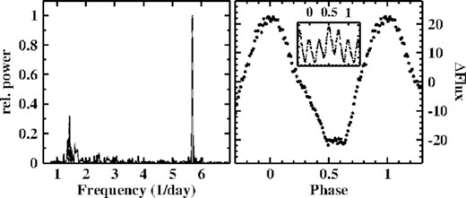
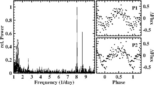
Top: Light curve of V704 And. Bottom left: Power spectrum of the light curve. The upper insert shows the region around the main peak on an expanded scale, with the orbital signal marked by an arrow. The lower insert contains the low frequency range (>2 d variations not removed). The arrow marks the beat between the strongly dominating signal at 6.7696 d−1 and the orbital frequency. Bottom right: Light curve folded on the period 0.147 72 d, binned in phase intervals of width 0.01.
The power spectrum (lower left frame of Fig. 1) is dominated by a very strong signal at 6.7696 (8) d−1.The first overtone is also seen, but is quite faint. The corresponding period of |$P_1 = 0.147\, 72\, (2)$| d is shorter than the spectroscopic orbital period |$P_{\rm WTH} = 0.151\, 424\, (3)$| d measured by Weil et al. (2018). The only other possibly significant signal (other than side lobes of the main one) is a much smaller peak at |$F_2 = 6.481\, (4)\, {\rm d}^{-1}$| (|$P_2 = 0.1542\, (1)$| d) (marked in the upper insert in the figure). This is closer to, but still markedly different from PWTH. The light curve, folded on P1 and binned in phase intervals of width 0.01 is shown in the right lower frame of Fig. 1. The waveform can well be approximated by a simple sine curve.
There is reason to suspect a misprint in period PWTH cited by Weil et al. (2018). Assuming that the third decimal digit in |$P_{\rm WTH} = 0.151\, 424$| d erroneously slipped in, we are left with |$P_{\rm WTH,corr} = 0.154\, 24$| which is identical to P2 within the error of the latter. This by itself is, of course, not sufficient evidence for an error. However, inspecting fig. 4 of Weil et al. (2018) it is obvious that the dominant peak in their periodogram is just below 6.5 d−1, compatible with 1/P2, but not with |$1/P_{\rm WTH}=6.603\, 97$| d−1. This lends more credibility to a misprint. Noting that the period of Weil et al. (2018) was derived from a longer time base than P2 and should thus be more precise, I will therefore henceforth adopt |$P_2 \approx P_{\rm WTH,corr} = P_{\rm orb} = 0.154\, 24\, (3)\, {\rm d}$| as the orbital period of V704 And.
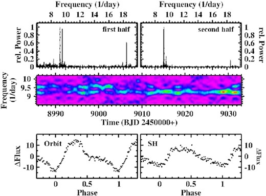
The dominant photometric period P1, coherent over the entire time base of the TESS observations, is thus distinctly different from the orbital period. These photometric variations therefore constitute a (negative, since P1 ≡ PSH < Porb) superhump.
Further investigation of the superhump signal confirms this interpretation. The lower frame of Fig. 2 shows the time resolved power spectrum in the frequency range around 1/PSH, constructed according to Bruch (2014), and using a sliding window of width 1 d. The power of the superhump signal is clearly modulated with time as quantified by the graph in the upper frame of the figure. The power spectrum of the latter contains a strong peak corresponding to 3.46 (5) d. Moreover, although not immediately apparent, the original data are also modulated at the same period, as evidenced by the low frequency part of their power spectrum (lower insert in the lower left frame of Fig. 1 where the corresponding frequency is marked by an arrow). The period is 3.48 (4) d which is fully compatible with the beat period of 3.49 (2) d between orbital and superhump periods.
Bottom: Time resolved power spectrum of a narrow frequency range around the superhump frequency in V704 And. Top: Power integrated over the width of the superhump signal in the lower frame.
3.2 TT Ari: Negative and positive superhumps simultaneously present
TT Ari, detected as a variable star by Strohmeier, Kippenhahn & Geyer (1957), is undoubtedly one of the best studied NLs. Its photometric history over the past 40 y has recently been scrutinized by Bruch (2019) who also provides ample references to previous work. It may therefore be surprising that TESS data can add yet new aspects to the rich photometric behaviour of this system. As a VY Scl type star TT Ari alternates between more common high states and occasional states of reduced brightness. The spectroscopically determined orbital period of 0.137 550 40 (17) d (Wu et al. 2002) causes a photometric modulation only during the deep low state (Bruch 2019). In the high state it has never been detected. Instead, the optical light is dominated by a permanent negative superhump with an average period of 0.132 95 d which slightly varies over time. This behaviour was, however, interrupted between 1997 and 2004, when the negative was replaced by a positive superhump with an average period of 0.149 07 d (see Bruch 2019, for details).
The TESS light curve of TT Ari, based on observations in two sectors in subsequent time intervals, is shown in the upper frame of Fig. 3. Apart from slight variations on longer time scales there appears to be a modulation with a period of just over 1 d. Therefore, in order to fully maintain these variations, for the subsequent frequency analysis the cutoff time scale of the Savitzky–Golay filter used to remove longer term variations (see Section 2) was increased from the usual 2 d to 5 d. The resulting power spectrum is reproduced in the middle frame of Fig. 3 where the insert show the same spectrum on an expanded vertical scale in order to enhance fainter structures. Apart from some low frequency noise 6 signals can unambiguously be identified. They are listed in Table 2.
Top: Light curve of TT Ari. Middle: Power spectrum of the light curve. The insert shows the same data on an expandend vertical scale. Bottom left: Light curve of TT Ari folded on the period of the negative superhump (black) and the beat period between negative and positive superhump (red), binned in phase intervals of width 0.01. Bottom right: The same, folded on the period of the positive superhump.
Significant signals detected in the power spectrum of TT Ari and their interpretation.
| Frequency (d−1) | Period (d) | Interpretation |
|---|---|---|
| |$F_1 = \phantom{1}0.9010 (5)$| | P1 = 1.1099(6) | F4 − F3 |
| |$F_2 = \phantom{1}1.8103 (16)$| | P2 = 0.5524(5) | 2F1 |
| |$F_3 = \phantom{1}6.6210 (10)$| | P3 = 0.15103(2) | Pos. superhump |
| |$F_4 = \phantom{1}7.5233 (2)$| | P4 = 0.132921(2) | Neg. superhump |
| F5 = 13.2393(20) | P5 = 0.07553(1) | 2F3 |
| F6 = 15.0468(20) | P6 = 0.066459(9) | 2F4 |
It is easy to interpret the different signals. F4 is by far the strongest. The corresponding period being very close to the average period of the negative superhump there is no doubt that it is due to this permanent modulation in TT Ari. A much fainter signal at F3 has a period just slightly above the range of periods measured when the positive superhump appeared between 1997 and 2004 (see table 3 of Bruch 2019). Knowing that the superhump periods are slightly variable, it is close at hand to identify F3 with TT Ari’s positive superhump. F1 ≈ F4 − F3 is then due to the beat between the negative and positive superhumps. F2, F5 and F6 are obviously the first overtones of F1, F3 and F4. The slightly asymmetric waveforms of the superhump and beat modulations are shown in the bottom frames of Fig. 3.
Representative eclipse epochs.
| Star | Light curve | Epoch (BJD) | Cycle number1 |
|---|---|---|---|
| AC Cnc | LC#1 | 2457179.2850 | 42895 |
| LC#2 | 2458281.1357 | 46562 | |
| LC#3 | 2459520.0024 | 50685 | |
| TV Col | LC#1 | 2458461.1377 | 52749 |
| LC#2 | 2459199.1453 | 55973 | |
| AQ Men | LC#1 | 2458340.2116 | 0 |
| LC#2 | 2458352.1133 | 791 | |
| LC#3 | 2458529.0722 | 1335 | |
| LC#4 (part 1) | 2458611.1237 | 1915 | |
| LC#4 (part 2) | 2458638.0025 | 2105 | |
| LC#4 (part 3) | 2458669.1256 | 2325 | |
| LC#5 (part 1) | 2459050.0996 | 5018 | |
| LC#5 (part 2) | 2459073.0176 | 5180 | |
| LC#6 | 2459156.0597 | 5767 | |
| LC#7 | 2459266.1223 | 6545 | |
| LC#8 (part 1) | 2459348.0324 | 7124 | |
| LC#8 (part 2) | 2459373.0721 | 7301 |
The remarkable feature of the TESS light curve of TT Ari is thus the simultaneous appearance of both, negative and positive, superhumps. This has never been seen before in this system. But in view of the strong difference in power of the respective power spectrum signals it is doubtful if the fainter positive superhump would be seen in terrestrial data sets, even if it were present simultaneously. Thus, both superhumps may have coexisted previously.
Concluding, I note that the power spectrum of TT Ari contains a broad range of enhanced power between 50 and 100 d−1 (corresponding roughly to periods between 15 and 30 min). Signals in this range have often been seen in the past (see Section 3.2 of Bruch 2019, and references therein) and are generally referred to as quasi-periodic oscillations (QPOs).
3.3 AC Cnc: A 4.6 d period
AC Cnc was detected as a variable star by Kurochkin (1960). Kurochkin & Shugarov (1980) first saw eclipses in the system and determined the orbital period which was last refined to be 0.300 477 47 (4) d by Thoroughgood et al. (2004) who also determined the orbital inclination i = 75.˚6 ± 0.˚7. The system thus belongs to the long period CVs. Slight period changes have been analysed by Qian et al. (2007). Soon after the detection of eclipses the nature of AC Cnc as a CV was disclosed in spectroscopic observations by Okazaki, Kitamura & Yamasaki (1982), and in the same year Downes (1982) detected the secondary star in the spectrum, making AC Cnc one of the few double-lined eclipsing variables among CVs and thus enabling the measurement of masses with a minimum of assumptions (see Schlegel, Kaitchuck & Honeycutt 1984; Thoroughgood et al. 2004). A limited amount of time resolved photometry of AC Cnc has been published by Yamasaki, Okazaki & Kitamura (1983).
TESS observed AC Cnc in two sectors in subsequent time intervals (LC#3). 6.5 and 3.5 yr before this epoch, the system was observed by the Kepler satellite in high cadence mode as part of the K2 mission (LC#1 and LC#2). All light curves are shown on the same time scale in Fig. 4. AC Cnc exhibits primary and secondary eclipses (see below). The primary eclipses are seen in the figure as a dense series of excursions to (almost) the same low flux level. The secondary eclipses cannot be resolved on the scale of the figure. The out-of-eclipse flux level shows significant variations on the time scale of days. These are not artefacts of the data reduction (see Section 2) since they also appear in the PDCSAP data.
Light curves of AC Cnc observed as part of the Kepler K2 mission (LC#1 and LC#2) and by TESS (LC#3), all drawn on the same time scale. The yellow graphs represent smoothed versions of the light curves after applying a Savitzky–Golay filter with a cut-off time scale of 17 d (primary and secondary eclipses masked).
The average waveform of the orbital variations of AC Cnc, based on 467 individual cycles, is shown in the upper left frame of Fig. 5. It is obvious from Fig. 4 that the depth of the primary eclipse increases with increasing system brightness. Therefore the light curves of individual orbital cycles were normalized before averaging such that the flux at eclipse minimum is 50 per cent of the mean flux in the phase intervals 0.2–0.3 and 0.7–0.8. Thus, the average only reflects the shape of the waveform, not the flux differences. Apart from the primary eclipse it is characterized by a secondary eclipse at phase 0.5 which interrupts sinusoidal variations with twice the orbital period and maxima close to phase 0.25 and 0.75. At the long period of AC Cnc it is expected (and confirmed by its imprint on the spectrum of the system) that the secondary star contributes non-negligibly to the total light. Considering also the red passbands of the TESS and Kepler satellites, the quasi-sinusoidal out-of-eclipse variations are readily interpreted as being due to ellipsoidal variations of the late type star. These variations as well as the secondary eclipse are not seen in earlier terrestrial light curves (e.g. Yamasaki et al. 1983) which were observed at shorter wavelengths.
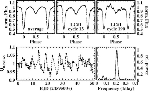
Top: Average waveform (left) of the orbital variations of AC Cnc normalized such that the eclipse minimum has 50 per cent of the average flux of the two maxima. The middle and right frames show examples of individual cycles where the brightness levels of the maxima before and after the secondary eclipse are significantly different. Bottom: Quotient of the average normalized flux in the phase intervals 0.2-0.3 and 0.7-0.8 for each cycle in LC#3 as a function of time (left) and the corresponding power spectrum (right).
However, this is not the whole story. The waveforms of individual cycles, as evidenced by the examples in the middle and right frames in the top row of Fig. 5, can exhibit a considerable difference in the flux of the orbital maxima. These do not occur at random. In the lower left frame of the figure the quotient Q2.5/7.5 of the average normalized flux in the phase intervals 0.2-0.3 and 0.7-0.8 of each cycle in LC#3 is plotted as a function of time. Q2.5/7.5 oscillates with a period of 4.79 (3) d as indicated by the power spectrum in the lower right frame of the figure. A similar, albeit fainter, oscillation of Q2.5/7.5 with a period of 4.77 (9) d is also seen in LC#2, but not in LC#1. It thus appears that a wave with a period just below 5 d modulates the light curves of AC Cnc.
Finally, I note a break in the gradient of the egress of the primary eclipse. Starting at phase ≈ 0.06 it becomes smaller. This feature, seen also in the eclipse shape of many other eclipsing CVs, indicates a non-axisymmetric brightness distribution of the eclipsed body, probably a hotspot at the disc edge.
The constancy of the flux level at eclipse minimum in spite of variations of the total system brightness indicates that these modulations occur in a part of the system which is totally eclipsed. Only when the brightness rises much above the average a small part of the extra light evades eclipse, causing a slight increase of the mid-eclipse flux (e.g. at BJD 2457190-95 in LC#1). On the other hand, the minimum flux of the secondary eclipse is proportional to the average out-of-eclipse flux (constant of proportionality: 0.9).
In particular in LC#3 the variations on time scales of days appear to show some regularity. To investigate this issue further, a Savitzky–Golay filter with a cut-off time scale of 17 d was applied to all light curves (masking both, primary and secondary eclipses), resulting in the smoothed light curves shown in yellow in Fig. 4. The difference between the original (again masking both eclipses) and the smoothed curves is shown in Fig. 6 (left) together with their low frequency power spectra (right). The power spectra of LC#2 and LC#3 clearly indicate the presence of a variation with a period of 4.73 (5) and 4.66 (2) d, respectively; identical within the error margin. The power spectrum of LC#1 contains several peaks, one of the strongest very close in frequency to the peaks seen in the other light curves and corresponding to a period of 4.63 (2) d. Least squares sine fits with periods fixed to the respective values are shown in yellow in Fig. 6. Is this the manifestation of the beat of orbital variations with some other periodicity? This is also suggested by the variations of Q2.5/7.5 in LC#2 and LC#3 which occur at the same periods. At higher frequencies, only the power spectrum of LC#3 contains a faint signal at 3.4305 (15) d−1, indicating the presence of a negative superhump with a period of 0.2924 (1) d. Otherwise, the power spectra of all light curves are strongly dominated by the orbital frequency and its overtones, which can clearly be identified up to the Nyquist frequency in the Kepler data (222th overtone!). No other significant signals are detected.
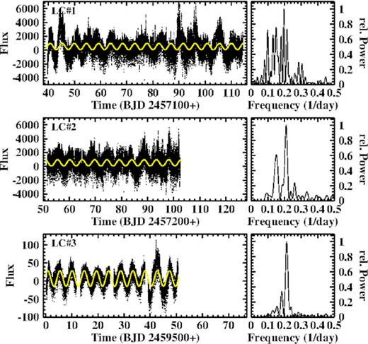
Left: Difference between the original light curves of AC Cnc (primary and secondary eclipses masked) and their smoothed versions (yellow graphs in Fig. 4). Right: Low frequency power spectra of the light curves. The yellow graphs on the left are least squares sine fits with the period fixed to the period of the dominant power spectrum signal (second highest peak in the case of LC#1).
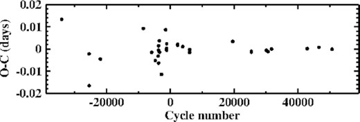
The orbital period of AC Cnc was last discussed in detail by Qian et al. (2007) who found a secular period decrease and suspected a superposed cyclic variation with a period of 16.2 yr. The current data permit to extend the time base for period determination significantly. Each of the light curves contain between 151 and 249 eclipses. Instead of measuring individual eclipse timings the light curves were folded on the orbital period choosing as epoch for the zero-point of phase an instant approximately in the middle of the light curve such that the centre of the primary eclipse coincides with phase 0. This yields the 3 high precision eclipse epochs for the three light curves listed in Table 3.
The O − C diagram is shown in Fig. 7. As expected the scatter is much higher for the photographically determined eclipse epochs (all data before cycle 0). At later epochs O − C is almost constant and close to 0. In particular, the presence of cyclic variations with a period of 16.2 y, suspected by Qian et al. (2007) based on the photoelectric/CCD O − C values and depending decisively on the single data point close to cycle 20 000, is not only not sustained by the present results but definitely ruled out. Thus, the conclusions drawn by them from the cyclic variations are obsolete.
O − C diagram of AC Cnc based on the ephemeris given in equation (1).
3.4 QU Car: Finally a more accurate orbital period
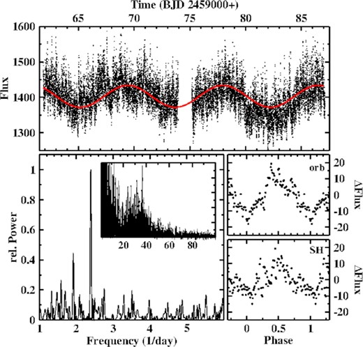
QU Car was discovered as an irregular variable by Stephenson, Sanduleak & Schild (1968) and classified as a cataclysmic variable by Schild (1969). At an average magnitude slightly fainter than 11 mag it is one of the brightest CVs in the sky. Currently considered to be a novalike variable, Kafka, Anderson & Honeycutt (2008) also proposed a classification as V Sge star, i.e. a system with characteristics similar to supersoft X-ray sources (Steiner & Diaz 1998). Despite its high brightness QU Car is a much less well studied system than many other much fainter CVs. Even the most basic of all binary parameters, the orbital period, is only know with a rather low precision. It was first determined spectroscopically by Gilliland & Phillips (1982) as 10.9 ± 0.3 h. While Kafka et al. (2008) did not see this period in their observations, it was later confirmed at an equally low precision by Oliveira et al. (2014). These authors also find a photometric modulation with the same period, but only when the flickering activity is reduced and the system hovers at a slightly lower magnitude level than normal.
The TESS light curve of QU Car is shown in the upper frame of Fig. 8. It is characterized by gradual variations with two well expressed maxima, separated by ≈38 d (the time base is evidently too short to affirm if they are periodic). This modulation is superposed upon variations on shorter time scales which are markedly stronger close to the maxima of the long term variations. While the eye does not clearly detect periodic variations on short time scale, this becomes different when modulations on time scales 2 d or longer are subtracted (second frame of Fig. 8). Regular variations are now unambiguously seen. The power spectrum of this light curve (lower left frame of Fig. 8) reveals irregular variations at frequencies <2 d−1 (very low frequencies are suppressed by the filtering process), and is dominated by a strong signal at F = 2.192 (1) d−1 (|$P=0.4563\, (2)\, {\rm d} = 10.951\, (5)\, {\rm h}$|) and its first overtone. This is obviously the orbital frequency and thus confirms and significantly improves the period found by Gilliland & Phillips (1982) and Oliveira et al. (2014).
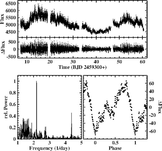
Top: Light curve of QU Car (upper frame) and the same after subtraction of variations on time scales longer than 2 d (lower frame). Bottom: Low frequency part of the power spectrum of QU Car, dominated by signals at the orbital frequency and the first overtone (left) and average waveform of orbital variations of QU Car (right).
Folding the data on the orbital period in order to determine the waveform and a fiducial structure to define a zero-point of phase is complicated by (i) strong flickering and (ii) the strongly varying amplitude of the orbital variations (second frame of Fig. 8). Assuming that the latter does not alter significantly the shape of the waveform this problem can be resolved by a proper normalization. For this purpose, I apply a spline fit to a manually defined approximate upper envelope of the orbital variations in the second frame of Fig. 8 and divide the light curve by the spline. Folding the results on the orbital period and binning them in phase intervals of width 0.005 then results in the average waveform displayed in the lower right frame of Fig. 8. It exhibits a gradual rise from a minimum (defined as phase 0) to a maximum at phase 0.75, and then a much quicker drop to the next minimum. This behaviour is quite similar to that observed by Oliveira et al. (2014) (see their fig. 11), meaning that QU Car did not change its waveform in the ≈9 years between the data sets.
Apart from the orbital signal, fainter isolated peaks in the power spectrum may hint at other persistent periodic modulations in the light curve. The most obvious of these is a pair of signals at 2.728 (2) d−1 and 2.774 (3) d−1 (corresponding to periods of 8.796 (8) h and 8.652 (7) h; see Fig. 8). These frequencies have no obvious relation to each other or to the orbital frequency. Time resolved power spectra revealed that the signals are mainly caused by variations during a few days close to the end of the observations, while at other intervals they are at most marginally present. Therefore, the evidence for them to be persistent is weak. Similarly, time resolved power spectra show that a candidate signal at higher frequencies (38.25 d−1) is not significant.
3.5 V504 Cen: A supraorbital period
Originally classified as a R CrB star (Kholopov et al. 1985), based on its spectrum Kilkenny & Lloyd Evans (1989) identify V504 Cen as a cataclysmic variable. The photometric behaviour made them suspect that V504 Cen belongs to the VZ Scl class. This was confirmed by Kato & Stubbings (2003) and Greiner et al. (2010) and even more impressively by the long term AAVSO light curve which – after a long sojourn in a high state – exhibits frequent and rapid successions of high and low states in recent years. Greiner et al. (2010) detected photometric variations in optical light, as well as in X-rays, and radial velocity variations which permitted them to determine an orbital period of 0.175 566 55 d.
TESS observed V504 Cen in a short intermediate state between two low states, about 1 mag below the normal high state. The light curves exhibits some irregular variations on the time scale of days which were subtracted to yield the power spectrum reproduced in the left frame of Fig. 9. It is dominated by a strong signal at the orbital frequency. At higher frequencies, only its first overtone is faintly present. The phase folded light curve in the right frame of the figure is characterized by a strong hump. Interestingly, it contains a constant interval between phase 0.485 and 0.635 (where the hump maximum defines phase 0). This gives the impression that the light source responsible for the orbital variations is temporarily blocked from view. In spite of having been observed at a similar wavelength this waveform is different from that obtained by Greiner et al. (2010) (see their fig. 2) when V504 Cen was in a genuine high state, and which has a flat topped maximum and a sharp minimum.
Left: Power spectrum of the light curve of V504 Cen. Right: Light curve of V504 Cen folded on the orbital period and on 4 times the orbital period (insert).
As an unusual feature the power spectrum of V504 Cen indicates the presence of another periodic signal at exactly 1/4 of the orbital frequency. The corresponding additional modulation of the brightness of the system at 4 times the orbital period is evident in the light curve, folded on this period, shown in the insert in the right frame of Fig. 9. Every third and fourth maximum is significantly brighter than the first and second. This odd behaviour cannot be explained by the presence of variations with independent periods (such as superhumps). I am not aware of other systems showing anything similar.
3.6 TV Col: The spin period finally detected in optical light
The intermediate polar TV Col was identified as the optical counterpart of the hard X-ray source 2H 0526-328 by Charles et al. (1979). It exhibits complicated photometric variations which include 3 periods observed in optical light, in addition to another period only seen in X-rays. The detection by Schrijver et al. (1985) of a 1938 s X-ray period, also claimed to have been seen in the UBV bands by Bonnet-Bidaud, Motch & Mouchet (1985), was later found to be ambiguous, the true period being 1911 s (Schrijver, Brinkman & van der Woerd 1987). A more accurate value of 1909.67 ± 2.5 s is provided in table 2 of Rana, Singh & Schlegel (2004). This period is interpreted as the rotation period of the WD, giving rise to the classification of TV Col as intermediate polar. It was never observed in the optical. Instead, optical variations occur at the spectroscopic period, considered to be orbital, first measured by Hutchings et al. (1981) and later refined to be 0.228 600 3 (2) d by Hellier (1993). Another shorter period modulation at 0.213 04 d, thought to be due to a negative superhump, is also often seen together with its beat with the orbit at 4.024 d (Motch 1981; Hutchings et al. 1981; Barrett, O’Donoghue & Warner 1988) and may be slightly unstable (Augusteijn et al. 1994). Hellier, Mason & Mittaz (1991) found shallow partial eclipses in the light curve of TV Col. Finally, Retter et al. (2003) claim to have seen a positive superhump with a period of 0.264 d.
Two TESS light curves of TV Col, separated by about 2 yr are avaialble and shown in the upper frames of Figs 10 and 11. LC#2 contains three short term outbursts (at BJD 2459194, 2459198 and 2459201) such as those observed by Szkody & Mateo (1984), Augusteijn et al. (1994) and Hudec, Šimon & Skalický (2005). They are ignored in the following analysis. It is obvious that the temporal behaviour of TV Col is quite different in the two light curves.
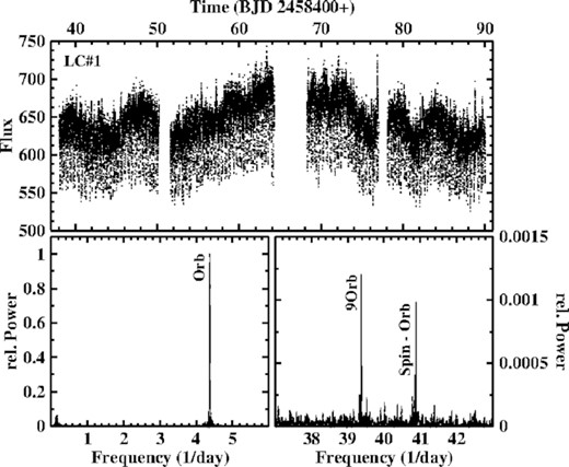
Top: Light curve LC#1 of TV Col. Bottom left: Low-frequency part of the power spectrum of LC#1 containing a strong signal at the frequency of the orbital variations. Bottom right: The same power spectrum at higher frequencies showing apart from an overtone of the orbital frequency a signal due to the beat between the orbital variations and variations caused by the spin of the WD.
The low frequency part of the power spectrum of LC#1 is shown in the lower left frame of Fig. 10. Apart from some very low frequency noise it contains only a single strong signal at the orbital frequency. No trace of the often seen superhump period at ≈4.63 d−1 or its beat with the orbital frequency is present. Thus, the superhump was definitely absent at the epoch of this light curve. A never before seen feature is revealed in the lower right frame of the figure which contains a small section of the power spectrum at higher frequencies. Apart from a high overtone of the orbital frequency a signal at 40.878 (2) d−1 is present which within the error margin is equal to Fspin − Forb = 40.87(6) d−1. It is thus the beat between the WD spin and the orbital period (i.e. the orbital sideband of the spin), a signal which is commonly seen in the light curves of intermediate polars instead of the spin period itself. This is the first time that a manifestation of the WD rotation period is seen in optical light of TV Col. The signal is also present in the power spectrum of LC#2.
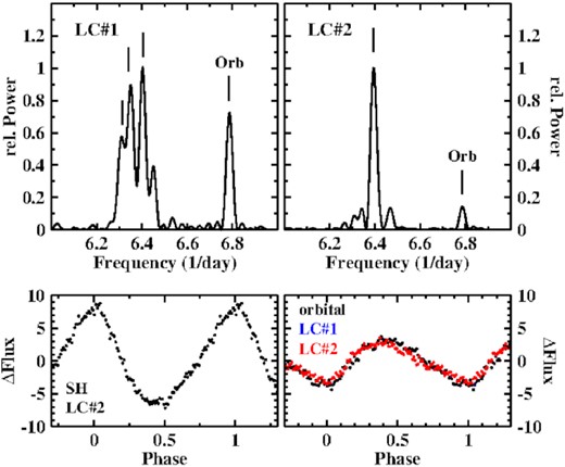
Otherwise, LC#2 behaves quite differently. The light curve contains obvious periodic variations on the time scale of days which immediately suggest to be due to the beat between the orbital and the commonly observed superhump period of TV Col. This is confirmed by the power spectrum, the low frequency part of which is reproduced in the lower left frame of Fig. 11. The superhump is again active at 4.6307 (3) d−1 (|$P = 0.215\, 95\, (1)$| d) and generates a stronger signal than the orbital variations. But the beat between the two at 0.2548 (4) d−1 (|$P = 3.894\, (5)$|) contains even more power. Linear combinations of FSH and Forb give rise to additional signals, as exemplified in the two other frames in the lower part of the figure.
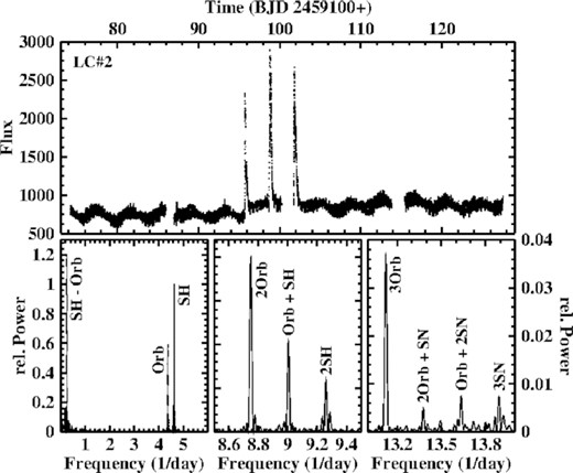
Top: Light curve of LC#2 of TV Col containing three short-term flares. Bottom left: Low frequency part of the power spectrum of LC#2, containing signals due to the orbital and negative superhump variations, as well as to the beat between them. Bottom middle and right: The same power spectrum at higher frequencies, showing examples of signals at linear combinations of the orbital and the superhump frequencies.
The occurrence of eclipses in TV Col, not easily discerned in individual cycles in terrestrial observations, is impressively confirmed when the light curves are folded on the orbital period. The waveform of the orbital variations is shown in the left frame of Fig. 12. For the first time, a secondary eclipse is also documented. While the waveform derived from LC#1 is approximately symmetrical, this is not the case for LC#2. It appears that, not surprisingly, the presence of the superhump light source implies in a significant change in the structure of the accretion flow in TV Col. To complete this issue the waveform of the superhump is shown in the right frame of Fig. 12.
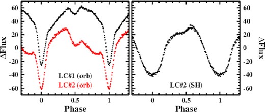
Left: Waveform of the orbital variations of TV Col of LC#1 (black, shifted vertically for clarity) and LC#2 (red). Right: Waveform of the negative superhump observed in LC#2.
3.7 DM Gem: Orbital and superhumps periods: which is which?
DM Gem is an old nova which erupted in 1903. Very few details of the underlying binary system are known. Lipkin, Leibowitz & Retter (2000) observed QPOs which they interpreted as a combination of two distinct signals with closely spaced periods near ∼2.95 h. Variations at the same period were also seen in photometric observations of Rodríguez-Gil & Torres (2005). They consider them to be probably linked to the orbital period. The latter authors also claim the presence of short-term variations on the time scale of ∼20 min.
The TESS SAP light curve of DM Gem contain some features such as systematically different flux levels in adjacent parts of the light curves, significant linear gradients or even apparent ‘outbursts’ which are clearly artefacts. All of these are absent in the PDCSAP data. Therefore, in this case, I prefer to use the latter.
The power spectrum of the light curve is shown in the left frame of Fig. 13. There is the usual forest of peaks at low frequencies caused by residual irregular variations on longer time scales. But dominating are two peaks at |$F_1 = 8.0495\, (8)\, {\rm d}^{-1}$| (|$P_1 = 0.124\, 23\, (1)\, {\rm d}$|) and |$F_2 = 8.0430\, (10)\, {\rm d}^{-1}$| (|$P_2 = 0.115\, 70\, (1)\, {\rm d}$|), the latter being somewhat fainter. The amplitude of these variations is quite small, such that the folded light curves, even after binning, are rather noisy, as seen in the two right hand frames of the figure. In both cases the waveform is sinusoidal. A time resolved power spectrum (not shown) reveals that the strength of the signal is quite variable and may remain below the detection level for intervals of days. This is particularly true for the P2 signal.
Left: Power spectrum of the light curve of DM Gem Right: Light curve of DM Gem folded on the periods P1 (top) and P2 (bottom), binned in phase intervals of width 0.01.
Within the error limits quoted by Rodríguez-Gil & Torres (2005) the period seen in their light curves is identical to P1. If this is the orbital period of DM Gem, it is close at hand to suspect P2 to be the period of a negative superhump. Or should it be vice versa, P2 being the orbital and P1 a positive superhump period? The period difference is 6.9 per cent. The average differences for negative and positive superhumps calculated from table 4 of Yang et al. (2017) is |$3.9 \pm 1.8{{\ \rm per\ cent}}$| and |$5.1 \pm 2.4{{\ \rm per\ cent}}$|, respectively. This may indicate a slight preference for P1 to be due to a positive superhump, but this is far from conclusive. To settle this question, a spectroscopic determination of the orbital period is required.
Beat frequencies and periods between Porb and P2, and calculated values for F2 = Forb − Fbeat and P2 based on LC#1 of V533 Her and its parts LC#11 (before the gap) and LC#12 (after the gap). The time unit is the day.
| LC#11 | LC#12 | LC#11 + LC#12 | |
|---|---|---|---|
| Fbeat | 0.378 (1) | 0.472 (3) | 0.443 (2) |
| Pbeat | 2.644 (9) | 2.12 (1) | 2.26 (1) |
| F2 | 6.407 (1) | 6.314 (2) | 6.343 (2) |
| P2 | 0.15607 (3) | 0.15838 (7) | 0.15766 (5) |
| LC#11 | LC#12 | LC#11 + LC#12 | |
|---|---|---|---|
| Fbeat | 0.378 (1) | 0.472 (3) | 0.443 (2) |
| Pbeat | 2.644 (9) | 2.12 (1) | 2.26 (1) |
| F2 | 6.407 (1) | 6.314 (2) | 6.343 (2) |
| P2 | 0.15607 (3) | 0.15838 (7) | 0.15766 (5) |
Apart from the P1 and P2 signals and the forrest at low frequencies a lonesame peak at 2.650 (2) d−1 (|$P = 0.3774\, (2)$| d) appears to have some significance. This period being very close to 3P1 may or may not be a coincidence. I cannot offer a viable explanation for this signal. At higher frequencies there are no indications for coherent or QPOs such as those seen by Rodríguez-Gil & Torres (2005) at ∼20 min.
3.8 RZ Gru: The orbital period and a superhump?
RZ Gru is a little studied novalike variable of the UX UMa subtype. Originally discovered as a variable star by Hoffmeister (1949) its nature as a cataclysmic variable was first suspected by Kelly, Kilkenny & Cooke (1981) and then confirmed by Stickland, Kelly & Cooke (1984). The orbital period is uncertain. In a short notice Tappert, Hanuschik & Wargau (1998) quote two possible values based on spectroscopic observations on September 29 and Ocober. 2, 1995 (0.360 d and 0.408 d) without indicating error limits.
The TESS light curve of RZ Gru is plotted in the upper frame of Fig. 14. On longer time scales it is characterized by a nearly sinusoidal variation. This is preserved in the PDCSAP data and is therefore probably real. A formal least squares fit (red graph in the figure) yields a period of 8.53 d. The power spectrum of the original light curve has a strong peak corresponding to a very similar period of 8.55 (13) d. Of course, more cycles have to be covered to be certain that this apparent period is persistent.
Top: Light curve of RZ Gru. The red curve is a least squares sine fit to the data with period of 8.53 d. Bottom left: Power spectrum of the light curve of RZ Gru. The insert shows a wider frequency range, containing a broad range of QPOs. Bottom right: Light curve of RZ Gru folded on the orbital (top) and the superhump (bottom) period, binned in phase intervals of width 0.01.
The power spectrum after subtracting variations on time scales >2 d is shown in the lower left frame of Fig. 14. It is dominated by a maximum corresponding to a period of |$P_1 = 0.4175\, (8)$| d. This is quite close to one of the two options quoted by Tappert et al. (1998) for the orbital period. They did not quote errors. But their observations were obtained in two nights spanning a time base of at most ≈3.5 d or ≈8.4 cycles. A period error equal to the difference between their period and P1 would therefore lead at most to a phase shift of 0.20. Depending on the unknown quantity and quality of the spectroscopic data a period error leading to a phase shift of this magnitude is not inconceivable. Therefore, I will assume P1 = Porb.
The beat frequency between the orbital and superhump period at 2.12 (4) is not seen in the power spectrum. Its period is also much smaller than the period of the strong 8.55 d modulation in the light curve. But is it a coincidence that within 0.5 times the propagated formal error the latter is an integer multiple (i.e. four times) of the former? A similar case has been observed by Bruch & Cook (2018) in V603 Aql, the brightness of which is modulated at exactly twice the beat period between orbit and superhump.
A final interesting feature is an enhancement of power at frequencies between roughly 20–65 d−1 (see insert in the lower left frame of Fig. 14) which may be considered a broad range of QPOs. A time resolved power spectrum reveals no persistent features in this range. This distribution of power is different from that of most other CVs where red noise caused by flickering leads to monotonous decrease of power towards high frequencies (see, e.g. Bruch 2022).
3.9 V533 Her: Superhumps with period variations
V533 Her is the remnant of a bright nova which exploded in 1963. The quiescent system gained some attention when Patterson (1979) observed coherent oscillations with a period of 63.3 s which appeared to indicate that the system belongs to the rapidly rotating intermediate polars of the DQ Her subclass. However, later observations by Robinson & Nather (1983) showed that these oscillations had disappeared, casting doubt on the magnetic rotator model for V533 Her. Unfortunately, the time resolution of the TESS data is not sufficient to resolve the corresponding period range and to investigate this issue further. A spectroscopic orbital period of |$P_{\rm orb} = 0.146\, 885\, 1\, (3)$| d or |$P_{\rm orb} = 0.147\, 374\, 3\, (3)$| d was measured by Thorstensen & Taylor (2000). A slightly shorter photometric period of 0.142 89 (2) d was observed by McQuillin et al. (2012) in SuperWASP data. It may be related to a negative superhump.
TESS observed V533 Her during two time intervals separated by about one year. After submission of the original version of this study Leichty et al. (2022) published a small paper on V533 Her based on the same TESS data. They used techniques similar to those applied here, but the approach for the interpretation of the observational results is slightly different.
The power spectra of the light curves are dominated by two signals between 6 and 5 d−1 as shown in upper frames of Fig. 15. The higher frequency peaks can readily be identified as being due to the longer of the two candidate orbital periods of Thorstensen & Taylor (2000) [see also Leichty et al. (2022)].
Top: Power spectra of the two light curves of V533 Her in a narrow frequency range around the dominating signals. Bottom: Waveforms of the superhump variations in LC#2 of V533 Her (left) and the orbital modulation in LC#1 and LC#2, plotted on the same scale.
In agreement with Leichty et al. (2022) I interpret the second signal as a positive superhump. In LC#1 it consists of several overlapping peaks at frequencies (collectively referred to here as FSH) between ≈ 6.25 and 6.50 d−1 in LC#1, but it has a simpler structure with a dominating peak at 6.3947 (7) d−1 in LC#2. In order to understand this behaviour a time resolved power spectrum of LC#1 was calculated, using a sliding window of width 2.6 d. The result is plotted as a function of time and frequency in the bottom frame of Fig. 16 (note that the difference in appearance of the corresponding power spectrum of Leichty et al. (2022) is exclusively due to the larger window used by them). The orbital signal appears and disappears with time in a regular pattern. The power of FSH is modulated similarly in time, but additionally in frequency, being shifted to higher frequencies whenever the orbital signal disappears. This behaviour suggests to be due to the interference of two perodic signals with different amplitudes. This is confirmed by tests with artificial light curves. A similar effect is also clearly seen in the power spectrum of Leichty et al. (2022) where it manifests itself as wiggles in both, the orbital and the superhump frequencies which obviously must not be interpreted as real variations in the former, and probably also not in the latter.
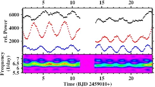
Properties of the power spectrum of LC#1 of V533 Her as a function of time. The lower frame shows the power on a colour scale as a function of time and frequency. The time interval affected by the gap between the two parts of the light curve has been masked. The upper frame contain the power integrated over three small frequency intervals (shifted vertically by an arbitrary amount for clarity). For details, see text.
But there is more to be extracted from the time resolved power spectrum. In the upper frame of Fig. 16 the integrated power in three small frequency intervals (from top to bottom: 6.20–6.44 d−1; 6.46–6.70 d−1, and 6.72–7.04 d−1) are plotted as a function of time (the graphs corresponding to the first two intervals have been shifted upwards by an arbitrary amount for clarity). The regular pattern seen in the time resolved power spectrum repeats, but the period is longer before the light curve gap and shorter afterwards. It appears that the change occurred within a short time interval. Interpreting the periods as the beat between Porb and PSH explains the main peaks of the FSH complex marked in Fig. 15, as is detailed in Table 4. This leaves only the third highest frequency peak in the FSH complex without an explanation.
Spectroscopic and photometric periods (in days) of CP Pup published in the literature. Errors of the last digits are quoted in parentheses if provided in the original paper.
| Spectroscopic period | |
| 0.06115 | Bianchini, Friedjung & Sabbadin (1985) |
| 0.061421 (25) | Duerbeck, Seitter & Duemmler (1987) |
| 0.06141 (3) | O’Donoghue et al. (1989) |
| 0.06148 (5) | O’Donoghue et al. (1989) |
| 0.061375 | Bianchini, Friedjung & Sabbadin (1990) |
| 0.06129 (1) | White, Honeycutt & Horne (1993) |
| 0.06126454 (9) | Bianchini et al. (2012) |
| 0.0614466 | Mason et al. (2013) |
| Photometric period | |
| 0.06196 | Warner (1985) |
| 0.06198 | O’Donoghue et al. (1989) |
| 0.06248 | O’Donoghue et al. (1989) |
| 0.06154 | O’Donoghue et al. (1989) |
| 0.0641 | Diaz & Steiner (1991) |
| 0.06834 (7) | White et al. (1993) |
| 0.061389 (5) | this paper |
Orbital, superhump and mutual beat periods (in days) identified in the TESS light curves of the target stars (literature values for the orbital periods are given whenever they are more accurate).
| Name | TypeA | Porb | PnSH | PpSH | Pbeat |
|---|---|---|---|---|---|
| V795 Her | SW | 0.1082648 (3)f | 0.10474 (1) | – | – |
| DM GemB | N (1903) | 0.11570 (1)a | – | 0.12423 (1) | – |
| DM GemB | N (1903) | 0.12423 (1)a | 0.11570 (1) | – | – |
| MV Lyr | VY | 0.1329 (4)g | 0.12816 (1)C | – | – |
| TT Ari | VY | 0.13755040 (17)c, D | 0.132921 (2) | 0.15103 (2) | 1.1099 (6) |
| AQ Men | UX | 0.14146835 (1)a | – | – | – |
| V533 Her | N (1963) | 0.147374 (5)e | – | 0.15645 (5) | – |
| V704 And | VY | 0.15424 (3)a, b | 0.14772 (2) | – | 3.49 (2) |
| V1193 Ori | UX | 0.165001 (1)h | 0.15883 (4) | 0.179922 (5) | – |
| TV Col | IP | 0.22860010 (2)a | 0.215995 (1) | – | 3.895 (5) |
| AC Cnc | UX | 0.30047747 (4)d | 0.2824 (1) | – | 4.65 (2) |
| RZ Gru | UX | 0.4175 (8)a | – | 0.520(2) | – |
| QU Car | UX | 0.4563 (2)a | – | – | – |
Notes.AN = nova (year or eruption); UX = UX UMa; VY = VY Scl; SW = SW Sex; IP = intermediate polar.
BTwo alternative interpretations.
CAverage from two light curves.
Dorbital period not detected in TESS data.
Considering the simpler structure of FSH in LC#2 a similar exersize for this light curve does not yield surprises. The time resolved power spectrum contains the same beat pattern, but this time the beat frequency does not change significantly over time. It yields a frequency of 6.392 (2) d−1 [|$P_2 = 0.156\, 45\, (5)$| d, marked in the right frame of Fig. 15], consistent with FSH.
The orbital and superhump waveforms (the latter only for LC#2 because of its period variation in LC#1), binned in phase intervals of width 0.01, are plotted in the lower frames of Fig. 15 on the same scale. The figure (i) confirms the larger amplitude of the superhump, (ii) reveals an asymetrical shape of both waveforms with a lower rise and quicker drop of the superhump and vice versa for the orbital modulation, and (iii) shows that the orbital waveform does not change neither in form nor in amplitude over the time scale of ≈1 yr.
The waveforms not being sinusoidal, overtones of the fundamental frequencies are expected in the power spectra. Indeed, several peaks (much fainter than the main signals) are seen at multiples of Forb and F2 and at simple arithmetic combinations. No other independent coherent periodicity could convincingly be detected up to the Nyquist frequency. In particular, just as Leichty et al. (2022) I see no trace of the negative superhump at |$P_{\rm nSH} = 0.142\, 89$| d seen in 2004 by McQuillin et al. (2012). It therefore must have vanished in the meantime. Finally, I mention that similar to the case of RZ Gru, an enhancement of power between roughly 35–80 d−1 indicates a broad range of QPOs in V533 Her.
3.10 V795 Her: First view of a negative superhump
V795 Her was discovered in the Palomar Green survey (Green et al. 1982) and initially suspected to be an intermediate polar (Shafter et al. 1990; Zhang et al. 1991; Thorstensen 1996). However, it appears now to be consensus that V795 Her is a SW Sex type novalike system as first proposed by Casares et al. (1996). With an orbital period of 0.108 264 8 (3) d determined spectroscopically by Shafter et al. (1990) it lies right within the period gap of CVs. V795 Her shows photometric variations with a slightly varying period, averaging 0.116 19 (7) d, somewhat longer than the spectroscopic period (see, e.g. Kalużny 1989; Patterson & Skillman 1994; Shafter et al. 1990; Papadaki et al. 2006; Šimon 2012), establishing the system as a permanent superhumper. Superposed upon the superhumps are rapid flickering variations and occasional QPOs with periods of 10–20 min (Patterson & Skillman 1994; Rosen et al. 1995; Papadaki et al. 2006).
The power spectrum of the TESS light curve is dominated by a signal at |$F_{\rm orb} = 9.2362\, (9)$| d−1 [|$P_{\rm orb} = 0.108\, 26\, (1)$| d], which is the orbital frequency, and a second one at a slightly higher frequency of |$F_{\rm nSH} = 9.547\, (1)$| d−1 [|$P_{\rm nSH} = 0.104\, 74\, (1)$| d] which I identify with a negative superhump. The first overtone of Forb is also present, but not of FnSH. However, the relative strength of the signals varies considerably over time. The upper frames of Fig. 17 contain the power spectra of the first (left) and the second half (right) of the entire light curve. While during the first half both signals have similar strength, the orbital signal is much stronger than the superhump signal during the second half. This is also obvious in the time resolved power spectrum reproduced in the middle frame of the figure.
Top: Power spectrum of the first (left) and second half (right) of the light curve of V795 Her. Middle: Time resolved power spectrum of the entire light curve Bottom: Waveform of the orbital (left) and negative superhump variations (right) of V795 Her.
Not a trace of the positive superhump, expected at 8.61 d−1 and seen in so many earlier observations, is present in the TESS data. On the other hand, a negative superhump has never before been reported in this system. The waveforms of the orbital and superhump variations are shown in the lower frames of Fig. 17.
Finally, I mention an enhancement of power in the broad frequency range of ≈65 − 125 d−1, consistent with the range of periods of QPOs reported previously.
3.11 HR Lyr: A 0.9 d modulation?
HR Lyr has erupted as a nova in 1919. The long term photometric behaviour of the system was studied by Leibowitz et al. (1995) on the base of 5 yr of observations. They found a 64 d modulation. Observing HR Lyr for even 22 yr, Honeycutt et al. (2014) could not confirm this period and discuss possible reasons for this discrepancy. Instead, they find sections of extended ascending or descending ramps in the brightness of HR Lyr. On nightly time scales, Leibowitz et al. (1995) claim the presence of QPOs around 0.1 h which they tentatively associate to an orbital period of about 2.4 h. However, it does not clearly reveal itself in the light curves. The featureless spectrum of HR Lyr (Kraft 1964; Williams 1983) makes it almost impossible to measure the orbital period spectroscopically. Thus, it remains unknown.
The TESS light curve of HR Lyr is reproduced in Fig. 18. It exhibits a slight rise over the 28 d time base which could be interpreted as a ramp as observed by Honeycutt et al. (2014). This notion is confirmed by a check of the AAVSO long-term light curve of the system. No periods are evident on a visual inspection.
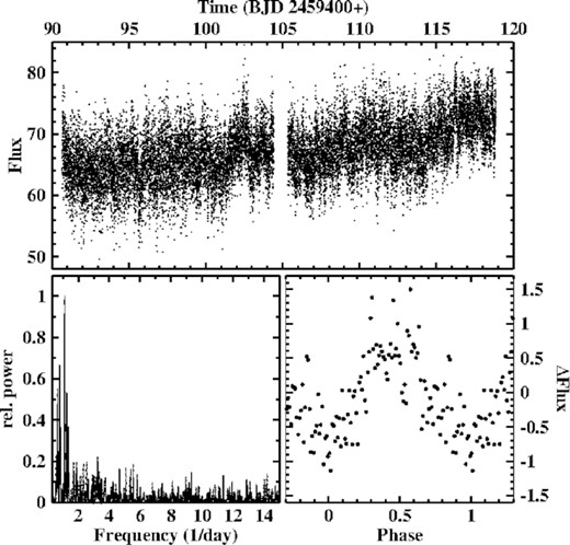
Top: Light curve of HR Lyr. Bottom left: Power spectrum of the light curve after removing variations on time scales >4 d. Bottom right: Light curve folded on the period 0.907 d.
The power spectrum (lower left frame of the figure) is almost featureless up to very high frequencies. In particular, there is no indication for the QPOs around F = 10 d−1 mentioned by Leibowitz et al. (1995). Only at quite low frequencies a peak at |$F = 1.102\, (4)$| d−1 (|$P = 0.907\, (3)$| d) stands out moderately high above surrounding peaks. Considering this signal tentatively to represent a real periodic variation of HR Lyr, the data folded on this period yield the quite noisy low amplitude waveform shown in the lower right frame of Fig. 18.
If real, could this period reflect the orbital motion? Probably not. At a period of just short of 1 d the secondary star should contribute a significant fraction of the system brightness and thus should readily be visible in the spectrum of HR Lyr. This is not the case not only when the system is on a relatively high brightness level as during earlier spectroscopic observations cited above, but also not when it was at a temporarily much reduced brightness of V ≈ 17 (Munari et al. 2016). Leibowitz et al. (1995) speculate about the presence of a third body in HR Lyr with an estimated orbital period of around 1 d and consider worthwhile the search of a corresponding periodicity. Identifying the 0.9 d period suggested here with the period predicted by them would pile speculation upon speculation. Thus, I just mention this possibility here without claiming it to a have a sound basis.
3.12 MV Lyr: First observation of a strong negative superhump
MV Lyr is a well studied NL of the VY Scl subtype. The orbital period has been determined spectroscopically by Voikhanskaya (1988), Borisov (1992) and last by Skillman, Patterson & Thorstensen (1995), but at 0.1329 (4) d it remains of rather low precision. MV Lyr also exhibits a slightly longer photometric period (Borisov 1992; Skillman et al. 1995) which may be interpreted as being due to a (positive) superhump. Periodic variations on longer times scales of near 3.8 d (Borisov 1992) and 3.6 (3) d (Skillman et al. 1995) were also reported but remain inconclusive because of the limited time base of the respective observations.
Three TESS light curves of MV Lyr are available. Vastly more observations were obtained by the Kepler satellite which monitored the star almost uninterruptedly in high cadence mode for just short of 4 years. These data are used here to complement the TESS data.
Starting the discussion with the Kepler observations, the entire light curve, binned in 1 d intervals for clarity, is shown in the upper frame of Fig. 19. For most of the time MV Lyr remained in a high state exhibiting gradual variations on the time scale of many days. For an interval of about 200 d between May and October 2011 the high state was interruped by a low state. Note that the considerable scatter of the average daily flux is not due to noise but reflects real brightness variations of MV Lyr on the time scale of a day.
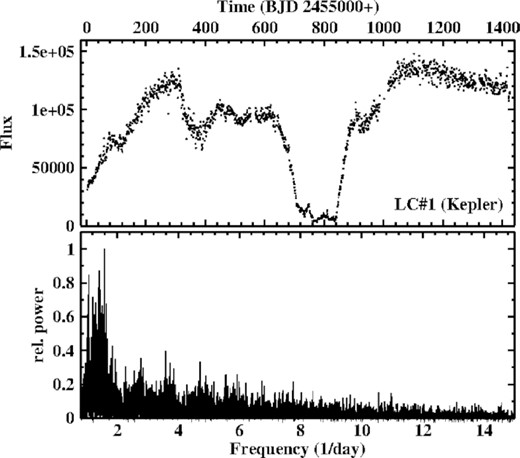
Top: Kepler light curve of MV Lyr binned in 1-d intervals. Bottom: Power spectrum of the light curve.
The power spectrum of the entire Kepler light curve is reproduced in the lower frame of Fig. 19. Is does not contain any outstanding signal which would indicate a persistent periodicity. Investigating smaller sections of the light curve, the power spectra sometimes contain marginally significant peaks, but they are not repeated in other sections and cannot be associated to previously observed periodicities. Instead, the power spectrum contains a wavelike structure with a dominant region of many peaks centred on ≈1.4 d−1, and other regions with decreasing power at integer multiples of the main range.
The power spectrum of LC#2 of the TESS observations (left frame of Fig. 20) is not unlike that of the Kepler data. The same, however, cannot be said of LC#3 and LC#4, the power spectra of which are totally different (right frame of the figure). They are dominated by a strong maximum at a very similar, but not identical frequency as is better seen when drawn on the expanded scale in the insert of the figure. In LC#3 the maximum peaks at |$F = 7.8120\, (8)$| d−1 (|$P = 0.128\, 01\, (1)$| d), in LC#4 at |$F = 7.7933\, (4)$| d−1 (|$P = 0.128\, 315\, (6)$| d). The period is thus slightly variable and about 3.5 per cent smaller than the orbital period, strongly suggesting that the signal is due to a negative superhump in MV Lyr. In both light curves the waveform (not shown) is very nearly sinusoidal.
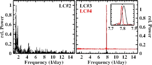
Power spectrum of TESS light curve LC#2 (left) and light curves LC#3 and LC#4 (right; the latter shifted vertically of clarity) of MV Lyr. The insert shows a small frequency range around the dominating peaks in order to emphasize their slightly different frequencies.
The change in behaviour of MV Lyr with no regular variations in LC#1 and LC#2 (before 2019, September) and the appearance of a very strong and never before seen negative superhump in LC#3 and LC#4 (after 2020, May) is remarkable. Moreover, neither the Kepler nor the TESS data contain any indication for the positive superhump observed by Borisov (1992) and Skillman et al. (1995). But both suspect a long term periodicity in their light curves. Is it a coincidence that the beat period between the orbital and the negative superhump period of MV Lyr is 3.63 d, very close the to the claimed long-term period suspected by them, but not detected in any of the present data?
3.13 AQ Men: An improved orbital period
AQ Men was detected in the Edinburgh-Cape Blue Object Survey as EC 05114-7955 by Chen et al. (2001) and classified as a cataclysmic variable. They suspected a dwarf nova nature but did not exclude the possibility of AQ Men being a novalike variable. Armstrong et al. (2013) prefer the latter classification based on the absence of observed outbursts even many years after discovery and the compatible spectrum. From radial velocity variations covering only 1.5 cycles Chen et al. (2001) derived a period of 3.12 h. In extensive photometric observations Armstrong et al. (2013) found a similar but more precise period of 0.141 471 (8) d and suspect the presence of grazing eclipses. They also found a supraorbital period of 3.78 d from which they inferred the presence of a negative superhump and which also causes a marginally significant peak in their power spectrum at 7.33 d−1.
3.14 V1193 Ori: Superhumps with variable waveforms
V1193 Ori was discovered by Hamuy & Maza (1986) who noted its similarity to CVs. This classification was confirmed by Bond et al. (1987) who showed that the system is a UX UMa-type novalike variable. A spectroscopic period measured by Ringwald, Thorstensen & Hamvey (1994) is consistent with the photometric period of 0.165 001 (1) d derived by Papadaki et al. (2006). However, while the latter authors did not see any other period in their data, Ak, Retter & Liu (2005) claim the presence of three different periods which they interpret as orbital [0.1430 d, assuming the periods of Ringwald et al. (1994) and Papadaki et al. (2006) to be 1/day aliases], a negative superhump (0.1362 d), and the beat between the other two periods (2.98 d).
TESS obtained two light curves of V1193 Ori, separated by about 2 yr. They show only small variation on time scales longer than days. On shorter time scales they contain clear variations which represent not only a challenge to reconcile them with the previous observations cited above, but are also drastically different during the two observing intervals. This is evident at first glance, regarding the power spectra of the two light curves in Fig. 21.
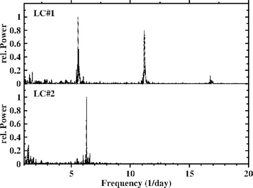
Power spectra of the two light curves of V1193 Ori.
In both power spectra some signals are seen at low frequencies which, however, do not have any relationship with other structures. I therefore consider them as being due to random variations on longer time scales. More importantly, LC#1 is dominated by a strong signal at |$F_1 = 5.580\, (1)$| d−1 [|$P_1 = 0.179\, 22\, (5)$| d]. Clear overtones at integer multiples of F1 are also present, but no other significant features. In contrast, LC#2 only contains a single strong line at |$F_2 = 6.296\, (1)$| d−1 [|$P_2 = 0.158\, 83\, (4)$|] with no overtones.
A closer look at LC#1 reveals another interesting feature. The light curve, after subtraction of variations on time scales >2 d, is shown in the upper frame of Fig. 22. A close inspection reveals even to the naked eye a regular pattern during the first ≈5 d. It reappears with a somewhat smaller amplitude after the gap in the light curve. In between this pattern is not readily apparent (shaded in the figure). In the time resolved power spectrum in the middle frame of Fig. 22 the otherwise strong F1 signal disappears during the highlighted part of the light curve. This can be explained, regarding the waveform of the variations responsible for F1. The lower part of the figure contains the three parts of the light curve, folded on P1 and binned in phase intervals of width 0.01. The zero-point of phase is the same in all three frames, chosen to coincide with the minimum of the waveform of the second half of LC#1 (after the gap). In the first and last part of LC#1 the waveforms are highly structured but differ only slightly. Apart from the difference in amplitude only a shift of the phase of the second maximum is significant. The width of the principle minimum varies slightly, but its phase remains the same. During the central part of the light curve, however, the waveform changes drastically to very nearly sinusoidal with a period P1/2 and extrema at different phases than before and after. The disappearance of F1 in the time resolved power spectrum is then explained by the doubling in frequency and the sinusoidal shape which shifts all power to 2F1. This is confirmed by the time resolved power spectrum around the first overtone of F1 (not shown).
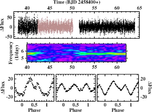
Top: LC#1 of V1193 Ori (after subtraction of variations on time scales >2 d) with a part exhibiting different temporal characteristics (see text) plotted in a lighter shade. Middle: Time resolved power spectrum in a narrow frequency range around the main signal at F1. Bottom: LC#1 folded on 1/F1 and binned in phase intervals of width 0.01: (left:) First part of light curve, (middle:) central (shaded) part, and (right:) final part.
In contrast, the waveform corresponding to the F2 signal in LC#2 is very nearly sinusoidal which explains the absence of overtones in the power spectra. F2 also appears in an independent data set. The AAVSO archives contain a series of light curves of V1193 Ori, observed in 8 nights between 2006, Jan 8–20. The power spectrum of the combined light curves (after subtracting the nightly average magnitude) has a strong peak at |$6.291\, (4)$| d−1, equal to F2 within the error limits. The waveform of the corresponding variations is also quasi-sinusoidal.
How to interpret the various periods of V1193 Ori found here and in the literature? Verifying the radial velocities listed in table 4 of Ringwald et al. (1994) I confirmed their spectroscopic orbital period and the inconsistency of their data with either P1 or P2. Using the on-line data provided by Papadaki et al. (2006) I also confirmed the presence of only the spectroscopic period in their measurements. In particular, the alternative orbital period of 0.1430 proposed by Ak et al. (2005) is incompatible with these data. Ak et al. (2005) based their analysis on a power spectrum with numerous peaks of similar height in the frequency range of interest (see their fig. 3). Their interpretation of structures corresponding to periods of 0.1430 d and 0.1362 d as orbital and as a negative superhump depends crucially on the assumption that the true orbital period is a 1/d alias of the value derived by Ringwald et al. (1994). Moreover, they calculate a probability of only 18 per cent that the alias period is correct. Taking into account also that the variations found by Papadaki et al. (2006) must then be considered as being due to a superhump which accidentally has a period exactly equal to the originally proposed orbital period, leaves little evidence for the period of Ringwald et al. (1994) to be wrong.
Coming back to the present data we then have a sequence |$P_1 = 0.176\, 223\, 8\, {\rm d} \gt P_{\rm orb} = 0.165\, 001\, {\rm d} \gt P_2 = 0.158\, 825\, 2\, {\rm d}$| and ∣P1 − Porb∣/∣P2 − Porb∣ = 0.550. This suggests that P1 is caused by a positive and P2 by a negative superhump in the light curve of V1193 Ori. But the variations seen by Ak et al. (2005) remain unexplained.
3.15 CP Pup: No ordinary old nova
Nova Puppis 1942 (CP Pup) was one of the brightest novae ever observed. Numerous studies have been dedicated to this system. Yet its nature is still shrouded in mysteries. Not only are the spectroscopic and photometric periods different from each other, but various authors found discrepant values at different epochs (see Bianchini et al. 2012, and references therein for a more detailed discussion). Mason et al. (2013) even raise doubts whether the radial velocity variations reflect the binary period at all or whether they might be caused by the rotation of a magnetic WD in a system with a longer orbital period. A summary of published period values is given in Table 5.
Two TESS light curves of CP Pup, separated by about 2 yr, are available. Some sections are evidently corrupted and/or contain short lived small scale outburst and were masked. The power spectra of both light curves are similar but differ drastically from those of all other stars in this study. They are dominated by a multitude of signals confined to the narrow frequency range between 14.3 and 17.0 d−1 (left-hand column of Fig. 23), corresponding to periods between 0.059 and 0.070 d, i.e. encompassing the range of photometric periods reported in the past. More signals on a 1.5 orders of magnitude lower power level occur at frequencies corresponding to the first overtone of this range (right-hand column of the figure). No other significant features were detected in the power spectra.
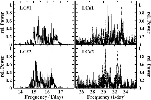
Power spectra of CP Pup.
Only one individual peak, and then the strongest one, repeats itself in both light curves at exactly the same frequency within the error limits. In LC#2 its first overtone can also clearly be identified, but not in LC#1. Its average frequency is |$F_1 = 16.290\, (1)$| d−1 [|$P_1 = 0.061\, 389\, (5)$| d]. The reappearence of this signal and the constancy of its frequency in two light curves separated by two years permits to presume that it is a persistent periodic variation in CP Pup.
The odd apparence of the power spectrum becomes more transparent if its time dependence is regarded. The second and third frames of Fig. 24 contain the time resolved power spectra of the two light curves in the relevant frequency range. A sliding window with a width of 4 d has been used to construct these spectra. Thus, structures within intervals of 4 d are not independent. The power spectra are characterized by a more or less continuous signal at F1, often interrupted or supplemented by other stronger and short-lived signals at neighbouring frequencies. Such intervals are readily identified in the light curves which are plotted above and below, respectively, the power spectra. Different states occur: Most of the time CP Pup remains in a state with a smaller amplitude of the variations (black dots in the figure) which I will call quiescence. However, this state is often interrupted by anomalous states of higher variability – the flaring states – which are highlighted by different colours. These flaring states coincide with the appearance of signals at frequencies other than F1 in the time resolved power spectra. In the lower frames of Fig. 24 the power spectra of only the quiescence (black) and the flaring states (using the same colour code as used in the light curves) are shown. It is obvious that the F1 signal is dominant in the quiescent state, while during flaring states variations at other frequencies prevail. The waveform of the variations is always very nearly sinusoidal.
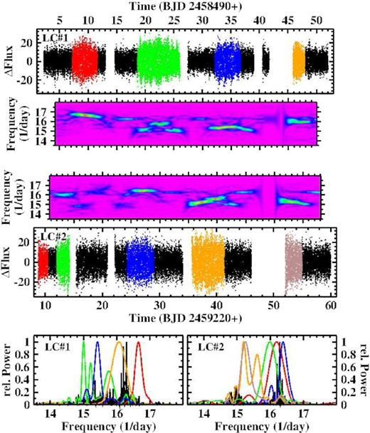
Time dependent behaviour of periodic variations in the light curves of CP Pup. The second and third frames contain the time dependent power spectra of light curves LC#1 and LC#2. The light curves are shown above and below, where quiescent and flaring states are drawn in black and in different colours, respectively. The power spectra of the different states are presented in the lower frames, using the same colour code as in the light curves.
The long and continuous TESS light curves of CP Pup for the first time permit a more comprehensive characterization of its photometric variation than was possible with the much more limited terrestrial data sets of the past. It appears clear that only one periodic signal at |$P_1 = 0.016\, 389$| d is persistent, although it may be suppressed during flaring states when variations at other periods become stronger. This period is close to published spectroscopic periods. It may thus well be the orbital period. But in view of the uncertainties in the interpretation of the spectroscopic data, I am reluctant to associate P1 definitely to the orbital period of CP Pup or the rotation period of the WD. Answering this and other deeper questions such as concerning the sudden appearance and disappearance of strong cyclic variations on a seemingly arbitrary period, albeit limited to a small and well defined period range, the physical origin of these always sinusoidal variations, or the reason for the period changes is beyond the scope of the present study.
The photometric behaviour of CP Pup is clearly different from that of any other CV. Although some of them sometimes exhibit bumps in their power spectra attributable to QPOs, these cannot be compared to the narrow and well defined range of periods and the strength of the signals seen here. Thus, citing the title of the paper of White et al. (1993): CP Puppis: No ordinary old nova.
4 SUMMARY AND OUTLOOK
The value of uninterrupted long duration and high time resolution photometric observations from space performed in particular by the Kepler and TESS missions not only but in particular for CV research has been demonstrated many times in the past. The current study can only confirm this obvious statement. In all of the 15 objects investigated here some new and sometimes surprising aspects have been found (although admittedly the current sample is biased due to the selection critera mentioned in Section 1). An abundance of superhumps, positive as well as negative, was detected, many of which have never been seen before. Some of them exhibit an interesting behaviour concerning their temporal development or their waveforms. Their periods are summarized together with some newly derived or improved orbital periods in Table 6, ordered according to increasing orbital period. There is no preference for superhumps to occur, or not to occur, among specific CV types or in a limited period range. It appears that negative superhumps are more common than positive ones, but this is not a statistically sound statement. Thus, the limited sample does not permit to draw clear and meaningful conclusions. A broader basis for a systematic accessment of superhumps in CVs other than outbursting dwarf novae is required. This is expected to be achieved by the extension of the current study, currently in progress as mentioned in the introduction, to more systems known to have exhibited superhumps in the past. A more thorough discussion, also taking into account the large amount of relevant information scattered in the literature, is therefore postponed to the follow-up study.
Even so, the availability of larger and better datasets already demonstrates that the occurrence of superhumps in NLs and old nova is not the exception as may have been expected in the past, but is a rather common feature in the light curves of these systems. Worthwhile mentioning is also the first detection in optical light of the WD spin period in TV Col in form of its orbital side band, and the curious time dependent frequency behaviour of CP Pup which explains the multitude of apparently contradicting periods reported in the past. Both results could not have been obtained easily by terrestrial observations.
This is an exploratory study. It has the purpose to identify interesting variations in the target stars and to document them. An in-depth investigation of their origin is left to subsequent work. There are many more CVs with TESS light curves which deserve to be scrutinized. The work is going on.
ACKNOWLEDGEMENTS
This paper is based on data collected by the TESS and Kepler missions and obtained from the MAST data archive at the Space Telescope Science Institute (STScI). Funding for the missions is provided by the NASA Explorer Program and the NASA Science Mission Directorate for TESS and Kepler, respectively. STScI is operated by the Association of Universities for Research in Astronomy, Inc., under NASA contract NAS 5-26555. Supportive data were obtained from the data arquives operated by the American Association of Variable Star Observers. I am grateful to Alexandre de Oliveira for his advice on the handling of TESS data.
All data used in the present study are publically available at the Barbara A. Mikulski Archive for Space Telescopes (MAST): https://mast.stsci.edu/portal/Mashub/clients/MAST/Portal.html and at the AAVSO web site: https://www.aavso.org.
