


ABSTRACT
Vega is the prototypical debris disc system. Its architecture has been extensively studied at optical to millimetre wavelengths, revealing a near face-on, broad, and smooth disc with multiple distinct components. Recent millimetre-wavelength observations from ALMA spatially resolved the inner edge of the outer, cold planetesimal belt from the star for the first time. Here we present early science imaging observations of the Vega system with the AzTEC instrument on the 32-m LMT, tracing extended emission from the disc out to 150 au from the star. We compare the observations to three models of the planetesimal belt architecture to better determine the profile of the outer belt. A comparison of these potential architectures for the disc does not significantly differentiate between them with the modelling results being similar in many respects to the previous ALMA analysis, but differing in the slope of the outer region of the disc. The measured flux densities are consistent between the LMT (single dish) and ALMA (interferometric) observations after accounting for the differences in wavelength of observation. The LMT observations suggest the outer slope of the planetesimal belt is steeper than was suggested in the ALMA analysis. This would be consistent with the interferometric observations being mostly blind to structure at the disc outer edges, but the overall low signal to noise of the LMT observations does not definitively resolve the structure of the outer planetesimal belt.
1 INTRODUCTION
Vega (HD 172167, α Lyrae) is a nearby, rapidly rotating A0 V star with a nearly pole-on orientation (Gulliver, Hill & Adelman 1994; Aufdenberg et al. 2006), located at a distance of 7.7 pc (van Leeuwen 2007), with an age of ∼400–850 Myr (Yoon et al. 2010). It was further revealed to be the host of a substantial circumstellar dust disc through detection of spatially extended, excess emission at mid- and far-infrared wavelengths by the InfraRed Astronomical Satellite (IRAS, Aumann et al. 1984). As the first such system to be identified, the Vega phenomenon presented some of the first tangible evidence for planetary systems around stars other than the Sun. Being the progenitor of this class of objects, the importance of understanding the structure and evolution of Vega’s debris disc cannot therefore be understated.
Interpretation of continuum emission from the circumstellar dust, i.e. its spectral energy distribution (SED), spanning infrared to millimetre wavelengths reveals the disc architecture to be best represented by a two-component disc. Spatially unresolved warm emission was identified at ∼ 20 au through Spitzer/IRS spectroscopy (Su et al. 2013), interior to an extended cool debris belt peaking at ∼ 90 au, revealed through imaging observations at longer wavelengths.
Imaging of the disc at millimetre wavelengths revealed a clumpy disc structure (Holland et al. 1998), prompting investigation of the potential for disc–planet interactions to induce dust trapping as a means to produce the observed non-axisymmetric emission (Wyatt 2003). Non-axisymmetric structure was also observed in subsequent observations (Wilner et al. 2002), leading to the interpretation of Vega having a disc perturbed by an unseen planetary companion. The subsequent detection of a clumpy ring in sub-millimetre images associated with a belt of dust-producing planetesimals at ∼ 85 au further reinforced this interpretation (Marsh et al. 2006).
The spatially resolved mid-infrared Spitzer (Su et al. 2005) and far-infrared images of Vega’s disc found that the disc is face-on, radially smooth out to several hundred au, but devoid of evidence for the clumpy substructure previously observed at millimetre wavelengths. The dust grains observed at infrared wavelengths are smaller and their motions more strongly subject to radiation pressure and stellar wind forces than larger grains seen at millimetre wavelengths. As such, they would not be expected to exhibit the same clumpy architecture.
Higher angular resolution far-infrared and sub-millimetre observations with the Herschel Space Observatory better constrained the cool, outer disc architecture as a broad ring lying at ∼ 100 au from the star, but the inner, warm component remained spatially unresolved (Sibthorpe et al. 2010). Subsequent re-investigation of the architecture of the disc at (sub-)millimetre wavelengths did not confirm the previous clumpy interpretation (Piétu et al. 2011; Holland et al. 2017), and interferometric measurements placed strict limits on the brightness and extent of any potential sub-structure in the Vega disc (Hughes et al. 2012). Most recently, ALMA Band 6 (1.34 mm) interferometric observations of Vega spatially resolved the outer cool belt for the first time, confirming its broad, smooth structure (Matrà et al. 2020).
The presence of two distinct components to Vega’s debris disc, as seen in continuum emission, brings into question the presence of planetary companions. The existence of planetary companions is often invoked to occupy the space between the two components (Kennedy & Wyatt 2014), analogous to the Solar system (Horner et al. 2020), but the origin of the inner warm component may be ambiguous (as is the case here). Direct imaging and radial velocity studies of Vega have so far turned up empty handed, with limits on companions of several Jupiter masses within 15 au of the star (Meshkat et al. 2018; Hurt et al. 2021).
A third component of emission from the Vega system has been identified through near-infrared interferometric measurements (Absil et al. 2013; Kirchschlager et al. 2018). This hot dust could originate from icy planetesimals transported inward through the system from the outer debris belt by planetary scattering (Raymond & Bonsor 2014). The observed hot dust component around Vega, if it originates from scattered planetesimals, can be sustained by a chain of five to seven low-mass planets located between the warm and cold components of the disc. It precludes the existence of high mass (≥MSaturn) planetary companions in the outer regions of the system as they would efficiently scatter inwardly migrating planetesimals out of the system entirely (Raymond & Bonsor 2014; Bonsor et al. 2018).
Spatially resolved, millimetre wavelength observations of a debris disc can be used to indirectly infer the presence of a planetary companion through dynamical interactions sculpting the dust-producing planetesimal belt. Sub-structure in broad debris discs around several stars has been identified and associated with the action of a planetary companion (e.g. Marino et al. 2018, 2019, 2020). Whilst the present observations of Vega are too coarse to infer the existence of sub-structure to the debris disc, one might still infer something from the overall shape of the belt (Kennedy 2020; Marino 2021). For example, a shallow outer slope to the debris belt at millimetre wavelengths could be indicative of a substantial high eccentricity, scattered population of planetesimals such as has been suggested for HR 8799 (Geiler et al. 2019). Previous ALMA observations of the Vega system have determined that the outer, cold planetesimal belt has a sharp inner edge and flat outer slope (Matrà et al. 2020). However, the interferometric nature of those observations were insensitive to the large scale structure of the outer planetesimal belt much beyond the peak of emission. To address the open question of the architecture of Vega’s cold debris disc, and search for evidence of planetary interaction with the belt, we obtained Early Science observations of Vega taken by the single dish, 32-m1 Large Millimeter Telescope (LMT) with the AzTEC instrument at a wavelength of 1.1 mm.
The remainder of the paper is laid out as follows. We present the new LMT observations and data reduction in Section 2. Section 3 is devoted to the relevant fundamental stellar parameters derived from ancillary data. We analyse the LMT image, measuring the disc flux density and comparing three radial profile models for the outer debris belt, in Section 4. We compare our findings to the recent study of the disc structure at millimetre wavelengths with ALMA in Section 5. Finally, we present our conclusions in Section 6.
2 OBSERVATIONS AND DATA REDUCTION
Observations of Vega were conducted in February and March of 2016 with the LMT and its 32-m configuration equipped with the 1.1 mm continuum AzTEC instrument (Wilson et al. 2008). The target was observed in small map mode, covering a region centred on the target and approximately 1.5 arcmin in radius to a uniform depth. A total of 8.8 h on source were devoted to observe the target under good to excellent weather conditions with an atmospheric opacity at 225 GHz of τ = 0.11 − 0.04. Pointing was secured through the bracketing observations of the Quasar 1801+440, approximately every hour. The analysis of pointing maps delivered an average of 1|${_{.}^{\prime\prime}}$|2 offset in right ascension and declination, which is well within the pointing uncertainty (≃ 2″) calculated for the entire observing season.
For the data reduction, we implemented a procedure similar to that already reported in Chavez-Dagostino et al. (2016) for the case of Epsilon Eridani, which is based on the processes described in Wilson et al. (2008) and Scott et al. (2008). Briefly, the reduction software takes into account the following aspects:
The first step corresponds to the raw time-stream signal conditioning and consists of cosmic ray and instrumental artefacts removal.
Next the atmosphere emission is calculated and subtracted by removing the largest eigenvalues in a principal component analysis (PCA) of the full array.
The cleaned signals are calibrated using a flux conversion factor (FCF) derived from daily beam map observations of CRL 618 and 3c273. In this step, the astrometric corrections to the telescope position signals are applied as well.
The time domain flux information is projected into a map using a weighted average of all the samples in a 1 × 1 arcsec2 pixel area.
The noise properties of the observation are estimated from a set of 100 simulated maps. These maps are constructed by multiplication of the cleaned timestreams with a random ±1 factor and projecting them into the same grid defined in step (iv).
To address any calibration systematic introduced by the data reduction algorithm, a 1 Jy synthetic point source is inserted into the raw time-streams and reprocessed by the pipeline. The output of this step along with the noise spectral density obtained in step (v) are used to construct an optimal Wiener filter for the observed map.
At this stage we avoid using the band-pass version of the filter used in extragalactic observations of point-like sources, instead we use a low-pass filter that allows us to preserve the extended emission around Vega. The filter allows us to increase the detectability of the astronomical emission at the cost of a slightly smearing of the angular resolution from the native 8|${_{.}^{\prime\prime}}$|5 to ≃ 11″.
2.1 Recovery of extended emission
When dealing with resolved sources, the atmosphere subtraction by PCA decomposition, is prone to modify the angular distribution of flux from astronomical sources. This effect is caused by the simultaneous detection of astronomical emission by multiple bolometers. In order to recover this missing flux, we use a modified version of the Flux Recovery Using ITerations algorithm (Fruit; Wall et al. 2016). The process starts by creating a binary mask over the map regions that exceed a threshold SNR > 3.0. Then, the mask is modified by a mathematical morphology closing operation followed by a dilation operation. The structuring element is a disc with a diameter of 11″. This operation removes from the mask structures smaller than the beam size. The mask is multiplied with the astronomical signal map and all pixels with negative flux values are removed. The result is known as the iteration map. The iteration map is mapped back to time domain and subtracted from the raw timestreams. This new timestreams are processed again by the reduction pipeline. The output map is considered a residual map. A total map is computed by adding the iteration and residual maps. The process is repeated over the total map until the maximum change between iterations is smaller than the noise level in the most current residual map. The comparison between the PCA and Fruit based reductions is shown in Fig. 1.

Azimuthal averaged radial profile comparison for the AzTEC reduction techniques. The blue squares show the output of the PCA based reduction, which is optimized for point-like sources. The profile shows a region of negative values from ≃ 25 to 60 arcsec. This region is the result of the oversubtraction of the atmosphere model to the astronomical emission. The red circles show the average radial profile recovered by the FRUIT technique. The profile exhibits higher values on scales larger than the beamsize and significantly reduces the oversubtraction effect.
3 STELLAR PARAMETERS
Vega is one of the most observed and well-characterized stars on the sky, being a primary calibration standard at optical wavelengths. Allende Prieto & del Burgo (2016) analysed the revised Hubble Space Telescope Space Telescope Imaging Spectrograph (STIS) absolute flux calibrated spectrophotometry for Vega. Their analysis yielded a good match between the best fitted Kurucz based synthetic spectrum and the observed data, as illustrated in their fig. 1, with the following free fundamental stellar parameters: the effective temperature Teff = 9485 ± 10 K, surface gravity log g = 3.94 ± 0.01 (with g in cm s−2), and iron-to-hydrogen abundance ratio [Fe/H] = −0.85 ± 0.01. These values are compatible with others from the literature, e.g. Royer et al. (2014) performed a thorough abundance analysis and spectral synthesis from high resolution, high signal-to-noise spectroscopy, resulting: Teff = 9550 ± 125 K, log g = 4.05 ± 0.20, and [Fe/H] = −0.41 ± 0.10.
Allende Prieto & del Burgo (2016) additionally determined the average angular diameter of Vega, θ = 3.333 ± 0.013 mas. The combination of this value with the Hipparcos parallax (Π = 130.23 ± 0.36 mas; van Leeuwen 2007) leads to an average linear radius R⋆ = 2.752 ± 0.013 R⊙. Note the adopted angular diameter perfectly agrees with the equatorial angular diameter obtained from high-precision interferometric measurements with the CHARA Array and the FLUOR beam combiner (θ = 3.33 ± 0.01 mas; Aufdenberg et al. 2006). Since Vega is a rapidly rotating pole-on star, it may be somewhat variable. For a more detailed discussion, see Allende Prieto & del Burgo (2016) and references therein.
The Bayesian inference code of del Burgo & Allende Prieto (2016, 2018) applied to the PARSEC v1.2S library of stellar evolution models (Bressan et al. 2012) has been proven to be painstaking and accurate enough from the statistical comparison with dynamical masses of detached eclipsing binaries. In particular, the predicted masses for main-sequence stars are, on average, within 4 per cent of accuracy (del Burgo & Allende Prieto 2018). We used this code taking as inputs the values of R⋆, Teff, and [Fe/H] from the aforementioned homogeneous analysis of Allende Prieto & del Burgo (2016), to derive the fundamental stellar parameters of Vega given in Table 1.
Fundamental stellar parameters of Vega. The radius, effective temperature, and metallicity were held as fixed values to infer the rest of parameters from the Bayesian code.
| Parameter | Value |
|---|---|
| Radius (R⊙) | 2.752 ± 0.013 |
| Effective temperature (K) | 9485 ± 10 |
| Metallicity [Fe/H] | -0.85 ± 0.01 |
| Mass (M⊙) | 1.9171 ± 0.0020 |
| Luminosity (log L/L⊙) | 1.7452 ± 0.0006 |
| Bolometric magnitude (mag) | 0.3770 ± 0.0015 |
| Mean density (g cm−3) | 0.0909 ± 0.0002 |
| Surface gravity (log g/cgs) | 3.8380 ± 0.0008 |
| Age (Myr) | 884 ± 4 |
4 MODELLING AND RESULTS
A cutout of the smoothed LMT/AzTEC 1.1 mm image centred on Vega is presented in Fig. 2. It has an effective resolution of 10|${_{.}^{\prime\prime}}$|9 (84 au, FWHM) and a continuum r.m.s. of 0.3 mJy beam−1. The whole map extends to around 90 arcsec in radius, roughly centred on the target position. The mapping is not uniform in coverage such that elevated noise levels are seen towards the map edges due to reduced coverage. However, for the region of interest in this work (the central ≈ 60″ diameter region), the coverage varies by 10 per cent from the centre of the map. Significant emission from the disc is detected out to 18″ (140 au), extending well beyond the peak of emission detected in the spatially resolved ALMA observations. Overall, the target emission is consistent with a spatially resolved face-on, axisymmetric disc detected at low signal-to-noise in its outer regions. We estimate the background level of the image using a circular annulus between 40 and 60 ″ from the stellar position.
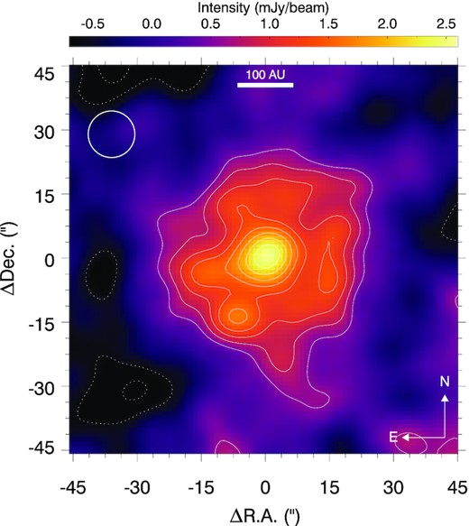
LMT/AzTEC 1.1 mm observation of Vega. The disc is seen to be face-on, extended, and smooth at the angular resolution of the telescope. Contours are from ±2-σ in increments of 1-σ, with negative contours as dotted lines, where the value of σ is calculated from the background variation of the map. Orientation is north up, east left. The instrument PSF (10|${_{.}^{\prime\prime}}$|9 FWHM) is denoted by the white circle in the upper left-hand corner.
In order to assess whether the disc is smooth, we consider a ring with inner and outer radii of 10|${_{.}^{\prime\prime}}$|9 and 23|${_{.}^{\prime\prime}}$|5 (83.7 and 180.5 au), with centre at the star position. The radius limits are chosen to include most of the disc emission at 1.1 mm, while avoiding the majority of the stellar flux: the inner limit is at two PSF standard deviations, while the outer value is the mean distance at which the disc flux has a 2-σ confidence level. We divide the ring along the azimuthal angle in slices 10° wide and compute the mean brightness for each slice. The results, shown in Fig. 3, invoke a smooth ring: a fit with a constant value provides a weighted average brightness of 0.0106 ± 0.0003 mJy arcsec−2 and a reduced chi square of 0.32, with a probability of the null hypothesis of 5.3 × 10⁻⁵. If we assume that the brightness difference of our data is real, a chi-squared test would reject the smoothness hypothesis if the error would be half (or lower) of that of the LMT observation. The signal-to-noise of the data in Fig. 3 implies that the ring is detected at, at least, a 3.9-σ level all along the azimuthal angle.
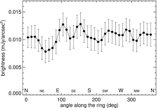
Azimuthal brightness distribution of the ring in the 10|${_{.}^{\prime\prime}}$|9–23|${_{.}^{\prime\prime}}$|5 distance interval from the star, uncertainties are 1-σ.
We model the cool debris disc as a face-on, radially smooth, and axisymmetric belt centred on the stellar position, following the findings from previous imaging observations (e.g. Su et al. 2005; Sibthorpe et al. 2010; Holland et al. 2017; Matrà et al. 2020). The disc inclination is therefore fixed as 0° in the models and the position angle of the disc is immaterial to the modelling. We examine three density radial profiles for the disc in comparison with the results of Matrà et al. (2020), namely a Gaussian ring, a single power law with sharp inner and outer edges, and a two power law model.
We generate disc density distributions for each profile in a 3D Cartesian volume encompassing the whole disc. Each disc model is scaled to the model disc flux density, the stellar flux is added to the central element of the volume, and the whole model is then convolved with a 2D Gaussian PSF model (FWHM 10|${_{.}^{\prime\prime}}$|9) to represent the instrument beam. The quality of the model as a fit to the observations is then evaluated through summation of the residuals (χ2) within 30 ″ (2 809 pixels, ≃ 20 beams) of the stellar position after subtraction of the convolved model from the observation. We multiply the observed noise by a factor |$\sqrt{A_{\rm beam}}$|, the square root of the beam area, in the χ2 calculation to take account of correlation between pixels due to oversampling of the beam by the image’s 1 arcsec pixel scale.
We determine the maximum-likelihood disc model parameters for each of the three model radial profiles using the Python-based Markov Chain Monte Carlo (MCMC) package emcee (Foreman-Mackey et al. 2013). The multidimensional parameter space is explored using 10 walkers per parameter over 500 steps (i.e. 40 walkers for the Gaussian model, 50 walkers for the power-law models). The walkers are initialized at values replicating the disc profiles derived from fitting the ALMA observations in Matrà et al. (2020), with an additional random scatter drawn from a uniform distribution with a width of 20 per cent of the nominal value (i.e. ±10 per cent). Due to the dynamic range we would usually adopt log10 values for the flux densities, radii, and widths. Instead the distributions are explored in linear space to avoid biasing the exploration towards smaller values as the data are weakly constraining (low angular resolution, low signal-to-noise). We determine the maximum likelihood and confidence intervals (16th and 84th percentiles) for all of the chosen parameters from the last 100 steps of the chains (i.e. 4000 or 5000 realizations of the model). The model fitting parameters and their uncertainties are presented in Table 2.
Disc modelling results.
| Model | |||
|---|---|---|---|
| Parameter | Gaussian | Power law | Two power law |
| f⋆ (mJy) | 1.7 ± 0.4 | 2.5 ± 0.3 | 2.6 ± 0.3 |
| fdisc (mJy) | 13.9 ± 1.3 | 13.2 ± 1.4 | 14.6 ± 1.6 |
| Rpeak (au) | 122 ± 2 | ... | 107 ± 5 |
| σR (au) | 46 ± 7 | ... | ... |
| Rin (au) | ... | 83 |$^{+7}_{-8}$| | ... |
| Rout (au) | ... | 232|$^{+26}_{-17}$| | ... |
| α | ... | −2.46|$^{+0.69}_{-0.76}$| | −4.08|$^{+0.30}_{-0.37}$| |
| γ | ... | ... | 6.87|$^{+2.01}_{-1.38}$| |
| χ2 | 20.5 | 20.5 | 20.9 |
All three model architectures tested here reproduce the observed emission with few significant residuals. We present the residual images subtracting the maximum-likelihood model for each architecture from the observation in Fig. 4. We find no substantial difference between the quality of fits for all three models tested in this work with similar χ2 values returned by the model fitting, as shown in Table 2.
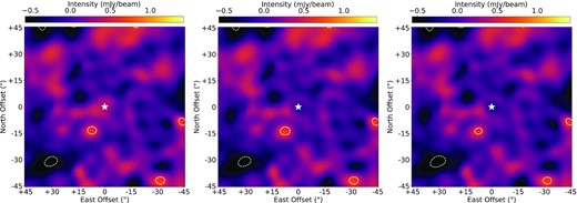
Plots of the residuals (i.e. observation - model) for the three disc architectures tested here. From left to right, they are the Gaussian, one power law, and two power-law models. The stellar position is denoted by the white ‘⋆’ symbol. Contours are in 1-σ increments from ± 2-σ, with negative values denoted by broken contours. The image colour scale is stretched between −2 and+ 5-σ.
5 DISCUSSION
The flux density of the mm-wavelength belt inferred by ALMA was model dependent due to the required extrapolation of the model to zero u, v separations (Matrà et al. 2020). With the single dish 32-m LMT/AzTEC, we measured the flux density of the outer belt to be around 14 mJy, and consistent across all three model architectures. Calculating the spectral slope of dust emission at millimetre wavelengths using measurements obtained with the James Clerk Maxwell Telescope (JCMT) (34.4 ± 1.6 mJy at 850 |$\mu$|m, Holland et al. 2017) and the Institut de Radioastronomie Millimétrique Plateau de Bure Interferometer (IRAM PdBI) (11.4 ± 1.7 mJy at 1.3 mm; Wilner et al. 2002) suggests that Vega’s debris disc should have a flux density around 18 mJy at 1.1 mm. This discrepancy could be resolved if there is some filtering in the map-making process of the data analysis that is removing flux, or that the background of the observed image is not flat and zero.
The stellar photospheric emission is found to be under 3 mJy in all three models. Extrapolation from shorter (near- and mid-infrared) wavelengths in the Rayleigh-Jeans tail of the stellar emission using the stellar parameters obtained in Section 3 predicts a photospheric contribution of around 3.5 mJy, significantly higher than the fitted value. The peak of the target emission, coincident with the stellar position, has a point source flux density of 2.4 mJy. We interpret this as additional evidence that the total emission from the system is being underestimated in these observations. If the background of the image were not flat, but bowled underneath the location of the disc, it would increase both the stellar flux density and the disc flux density.
The disc modelling results are also limited by the low angular resolution of the LMT observations (10|${_{.}^{\prime\prime}}$|9 FWHM). This is exemplified by the large uncertainty in the disc outer radius, Rout, for the one power-law model, and the large uncertainty for the inner power-law exponent, γ, for the two power-law model. Despite the limitations, the results for the disc architecture obtained here are consistent with the higher angular resolution ALMA observations in most regards (Matrà et al. 2020).
6 CONCLUSIONS
We have observed Vega, the prototypical debris disc system, at 1.1 mm with LMT/AzTEC. We resolve the outer belt of the disc, finding its architecture to be smooth and face-on, consistent with previous observations. A comparison of three potential surface brightness profiles for the belt (Gaussian, one and two power law) show that all three are consistent with the LMT/AzTEC observations, which we attribute to the low angular resolution (particularly of the inner extent of the cold planetesimal belt), and low signal-to-noise (≤ 5-σ) of the large-scale extended emission from the disc. The maximum probability models for each architecture fitted here are consistent, within uncertainties, with previous results for the same architectures presented in Matrà et al. (2020).
We confirm here the sharp inner edge of the planetesimal belt revealed in that work. This is inconsistent with models of the disc that invoke self-stirring within a broad belt of planetesimals to reproduce the observed emission, which would induce a flatter slope to the disc’s inner edge. It may therefore interpreted as indirect evidence of sculpting by a massive planetary companion interior to the disc.
However, the shape of the outer edge of the planetesimal belt remains poorly constrained. ALMA observations suggested the disc outer surface brightness profile was relatively flat, but the interferometric measurements were blind to disc structure beyond ∼ 140 au from the star. In contrast, the LMT observations suggest a very steep outer edge to the disc; such a narrow belt structure should reasonably have been detected in the ALMA observations. LMT/AzTEC image processing artificially steepens the slopes of extended structures in the image, this partially accounts for the discrepancy between our measurements and the ALMA-based analysis.
Future observations with appropriate large scale single dish millimetre-wavelength facilities such as the proposed Atacama Large Aperture Submillimeter Telescope (AtLAST; Klaassen et al. 2020), or the full 50-m LMT using the soon to be commissioned TolTEC instrument (Wilson et al. 2020; Lunde et al. 2020) will have a greatly increased angular resolution (≃ 5″ FWHM at 1.1 mm), and a substantially higher sensitivity, providing commensurately better constraints on the architecture of the cool debris disc. These unique capabilities will be essential to answer the still open question of the extent and outer slope of Vega’s cold planetesimal belt.
ACKNOWLEDGEMENTS
This research has made use of the SIMBAD data base, operated at CDS, Strasbourg, France (Wenger et al. 2000). This research has made use of NASA’s Astrophysics Data System.
FK and JPM acknowledge research support by the Ministry of Science and Technology of Taiwan under grant MOST107-2119-M-001-031-MY3, and Academia Sinica under grant AS-IA-106-M03. JPM acknowledges research support by the Ministry of Science and Technology of Taiwan under grant MOST109-2112-M-001-036-MY3. MC thanks Consejo Nacional de Ciencia y Tecnología (CONACyT) for financial support through grant CB-2015-256961.
Facilities: Large Millimeter Telescope.
Software: This paper has made use of the Python packages astropy (Astropy Collaboration 2013, 2018), scipy (Virtanen et al. 2020), numpy (Harris et al. 2020), matplotlib (Hunter 2007), and emcee (Foreman-Mackey et al. 2013).
DATA AVAILABILITY
The data and analysis scripts underlying the results presented in this article are available through a public repository on GitHub.
Footnotes
The LMT operated with its inner 32 m diameter until 2018. Since then, the LMT works with the full 50-m dish aperture.
