


ABSTRACT
Photospheric abundances of C, N, O, and Na were determined by applying the synthetic spectrum-fitting technique to 34 snap-shot high-dispersion spectra of 22 RR Lyr stars covering a metallicity range of |$-1.8 \lesssim$| [Fe/H] |$\lesssim 0.0$|, with an aim of investigating the mixing mechanism in the interior of low-mass giant stars by examining the abundance anomalies of these elements possibly affected by the evolution-induced dredge-up of nuclear burning products. Special attention was paid to check the recent theoretical stellar evolution simulations indicating the importance of thermohaline mixing in low-mass stars (|$M \lesssim$| 1 M⊙), which is expected to be more significant as the metallicity is lowered. By inspecting the resulting abundances in comparison with those of unevolved metal-poor dwarfs at the same metallicity, the deficiency in C as well as enrichment in N was confirmed (while O is almost unchanged), the extent of peculiarities tending to increase with a decrease in [Fe/H]. Accordingly, the [C/N] ratio turned out to progressively decrease towards lower metallicity from ∼0 ([Fe/H] ∼0) to ∼−1 ([Fe/H] ∼−1.5), which is reasonably consistent with the theoretical prediction in the presence of thermohaline mixing. However, these RR Lyr stars do not show any apparent Na anomaly (i.e. essentially the same [Na/Fe] versus [Fe/H] trends as those of dwarfs), despite that metallicity-dependent overabundance in Na is theoretically expected for the case of non-canonical mixing. This inconsistency between C/N and Na may suggest a necessity of further improvement in the current theory.
1 INTRODUCTION
After a star in the core hydrogen-burning phase (main sequence) has exhausted its central fuel, it begins to move towards the red giant stage in the Hertzsprung–Russell (HR) diagram while decreasing the surface temperature (Teff) as well as increasing the luminosity (L). Because of the deepening of convention zone caused by the reduction of Teff, the H-burning product in the interior can be salvaged into the surface by this enhanced mixing, by which the surface chemical composition of red giants tends to show characteristic anomalies due to the contamination of nuclear-processed material. For example, an appreciable C-deficiency as well as N-enrichment (while O is much less susceptible) would result by mixing of CNO-cycle products and a moderate overabundance of Na may arise due to NeNa-cycle products. Likewise, 12C/13C isotope ratio as well as Li or Be abundances may also serve as useful indicators. Yet, such an evolution-induced enhancement of convective dredge-up (standard mixing) is not the only mechanism that would take place in the stellar interior. It has been often argued (see e.g. Lagarde et al. 2012b and the references therein) that other non-canonical mixing processes may be significant depending on situations; such as rotation-induced mixing (meridional circulation or shear instability) and thermohaline mixing (instability induced by molecular weight inversion created by 3He + 3He → 2p + 4He reaction in the external wing of the H-burning shell).
Especially, the importance of thermohaline mixing on the surface composition is theoretically expected for the case of low-mass (|$M \lesssim 1 \, {\rm M}_{\odot }$|) metal-poor giants, because this process becomes more efficient as the initial mass decreases and the metallicity is lowered. This is demonstrated in fig. 6 or fig. 8 of Lagarde et al. (2019), where the simulated [C/N] (C-to-N abundance ratio) is plotted against [Fe/H] (metallicity).1 It is evident from their figures that the [C/N] versus [Fe/H] relations computed for the two cases of [1] standard mixing and [2] non-canonical mixing (including thermohaline mixing)2 are markedly different from each other; that is, while |[C/N]| (the extent of mostly negative [C/N]) tends to be gradually decrease with a decrease in [Fe/H] (i.e. mixing is suppressed as metallicity is lowered) in the former canonical case, a sequence of increasing |[C/N]| towards lower [Fe/H] ([C/N] decreases from ∼−0.5 to ∼−1 with a reduction of [Fe/H] from ∼0 down to ∼−1; which means an enhanced mixing with decreasing metallicity) newly appears in the latter non-canonical case.
Actually, Lagarde et al. (2019) showed in their fig. 8 that observed [C/N] values of red giants in several metal-poor open clusters (down to [Fe/H] ∼−1) appear to be more consistent with the latter trend than the former one, which suggests that thermohaline mixing may play the dominant role (over the standard mixing) in the metal-poor regime. However, since red giant stars in a cluster have various masses and evolutionary stages (but with almost the same age and metallicity), they are not necessarily adequate to study how the efficiency of mixing depends upon metallicity. As a matter of fact, the observed [C/N] values within the same cluster plotted in fig. 8 of Lagarde et al. (2019) are considerably diversified (presumably due to the differences in stellar parameters). Although Lagarde et al.’s (2019) theoretical population-synthesis calculations for the expected surface [C/N] ratios take into account such parameter differences of individual stars, it is rather difficult to compare these theoretical [C/N] versus [Fe/H] distributions with those derived from stars of open clusters, which have large dispersions and are available at only several ‘discrete’ [Fe/H] values.
In this context, it may be worth paying attention to RR Lyr stars, which belong to the class of horizontal-branch (HB) stars (post red-giant stage after the He-ignition) currently crossing the Cepheid instability strip. These pulsating variables may serve as an adequate testing bench for investigating the metallicity dependence of mixing based on their surface compositions for the following reasons. (i) They are low-mass stars (|$M \lesssim 1 \, {\rm M}_{\odot }$|; typically around |$\sim 0.8\, {\rm M}_{\odot }$|) and have effective temperatures in a rather narrow range (Teff ∼ 6000–7500 K), which means that they are similar in terms of stellar parameters and evolutionary stages. (ii) Meanwhile, their metallicities distribute in a sufficiently wide range (|$-2 \lesssim$| [Fe/H] |$\lesssim 0$|), which makes them suitable for studying the metallicity effect.
Very recently, an interesting report following this line has been made by Andrievsky et al. (2021). They determined the C, N, and O abundances of nine field RR Lyr stars, and found that the resulting [C/N] ratios tend to decrease towards lower metallicity from [Fe/H] ∼0 down to ∼−2 (cf. fig. 8 therein). This tendency is almost consistent with the simulation of Lagarde et al. (2019), supporting the importance of thermohaline mixing in low-mass giants. However, since Andrievsky et al.’s (2021) analysis is limited to only nine stars, their conclusion needs to be confirmed based on a larger sample of RR Lyr stars.
Conveniently, useful spectral data of some 20 RR Lyr stars applicable to this purpose are available, which were observed by the author’s group ∼20 yr ago. A part of these data for the specific four stars (for each of which several observations at different times were made) were first analysed by Takeda et al. (2006; hereinafter referred to as Paper I) in order to check the consistency of O and Fe abundances (and the reliability of spectroscopically established atmospheric parameters) determined from the spectra of different pulsation phases. Successively, based on all the available data, Liu et al. (2013; hereinafter Paper II) determined the abundances of 15 elements (Na, Mg, Al, Si, Ca, Sc, Ti, V, Cr, Mn, Fe, Ni, Cu, Y, and Ba) for 23 RR Lyr stars, though light elements such as CNO were outside the scope of their study.
Accordingly, in order to provide an independent follow-up study after Lagarde et al. (2019) and Andrievsky et al. (2021), it was decided to newly determine the photospheric abundances of four key elements (C, N, O, and Na) for this sample of RR Lyr variables (covering the metallicity range between [Fe/H] ∼−2 and ∼0), where the main attention is paid to clarifying the trend of [C/N] in terms of metallicity. This is the purpose of this investigation.
2 PROGRAMME STARS AND OBSERVATIONAL DATA
The observational materials used in this study are the 34 high-dispersion spectra of 22 RR Lyr stars (repeated observations were done for four stars: DH Peg, DX Del, RR Lyr, and VY Ser), which were obtained on 2004 June 27 (UT) by using the High-Dispersion Spectrograph (HDS) on the Nasmyth platform of the 8.2 m Subaru Telescope atop Mauna Kea. See Section 2 of Paper I for more details on the observations. The list of these 22 programme stars along with their observational times (Julian day) is presented in Table 1. Besides, additional information (e.g. pulsation period, phase, radial velocity, etc.) is given in table 1 of Paper II, which describes essentially the same data as adopted in this paper (except that two spectra of V445 Oph analysed in Paper II were discarded in this investigation as remarked in Section 3).
Atmospheric parameters of the program stars and the resulting abundance ratios.
| Star | HJD | Teff | log g | vt | [Fe/H] | [C/Fe] | [N/Fe] | [O/Fe] | [Na/Fe] | [C/N] | Remark |
|---|---|---|---|---|---|---|---|---|---|---|---|
| (1) | (2) | (3) | (4) | (5) | (6) | (7) | (8) | (9) | (10) | (11) | (12) |
| AA Aql | 2453184.955 | 6550 | 2.87 | 2.8 | −0.36 | −0.15 | + 0.30 | + 0.39 | + 0.07 | −0.45 | |
| AO Peg(1) | 2453185.031 | 6180 | 2.19 | 3.1 | −1.23 | −0.47 | (−0.09) | + 0.62 | −0.55 | (−0.38) | |
| AO Peg(2) | 2453185.039 | 6290 | 2.67 | 3.3 | −1.16 | – | – | + 0.77 | −0.54 | – | |
| BR Aqr | 2453185.011 | 6440 | 2.42 | 2.8 | −0.78 | −0.24 | + 0.46 | + 0.53 | + 0.03 | −0.70 | |
| CI And | 2453185.094 | 6380 | 2.72 | 2.8 | −0.39 | −0.14 | −0.04 | + 0.19 | −0.23 | −0.10 | |
| CN Lyr | 2453184.825 | 6380 | 2.98 | 3.2 | −0.08 | −0.16 | + 0.07 | + 0.04 | −0.12 | −0.23 | |
| DH Peg(1) | 2453184.962 | 7780 | 2.85 | 1.7 | −1.05 | −0.36 | + 0.71 | + 0.46 | −0.03 | −1.06 | Paper I |
| DH Peg(2) | 2453185.048 | 6990 | 2.69 | 1.7 | −1.21 | −0.23 | + 0.72 | + 0.56 | + 0.02 | −0.96 | Paper I |
| DH Peg(3) | 2453185.121 | 7110 | 2.79 | 1.7 | −1.23 | −0.26 | + 0.85 | + 0.60 | + 0.07 | −1.11 | Paper I |
| DM Cyg | 2453184.988 | 6400 | 2.88 | 3.1 | + 0.02 | −0.14 | −0.13 | + 0.02 | −0.10 | −0.01 | |
| DO Vir | 2453184.779 | 6340 | 2.63 | 2.0 | −1.24 | + 0.07 | + 0.78 | + 0.49 | + 0.22 | −0.71 | |
| DX Del(1) | 2453184.893 | 6670 | 2.63 | 3.1 | −0.21 | −0.09 | −0.02 | + 0.11 | −0.13 | −0.07 | Paper I |
| DX Del(2) | 2453184.980 | 6340 | 2.63 | 3.0 | −0.26 | −0.04 | −0.06 | + 0.06 | −0.07 | + 0.03 | Paper I |
| DX Del(3) | 2453185.069 | 6260 | 2.69 | 3.4 | −0.22 | −0.01 | −0.18 | + 0.12 | −0.06 | + 0.17 | Paper I |
| IO Lyr | 2453184.902 | 6350 | 2.11 | 2.8 | −1.39 | −0.47 | (−0.38) | + 0.54 | −0.37 | (−0.09) | |
| KX Lyr | 2453184.910 | 6580 | 2.91 | 2.8 | −0.30 | −0.09 | + 0.21 | + 0.11 | + 0.00 | −0.30 | |
| RR Cet | 2453185.083 | 6720 | 2.36 | 2.7 | −1.33 | −0.27 | + 0.48 | + 0.72 | −0.12 | −0.76 | |
| RR Lyr(1) | 2453184.796 | 7530 | 2.80 | 1.9 | −1.31 | −1.03 | + 0.27 | + 0.81 | −0.03 | −1.30 | Paper I |
| RR Lyr(2) | 2453184.882 | 6710 | 2.36 | 3.1 | −1.41 | −0.47 | + 0.21 | + 0.62 | −0.17 | −0.68 | Paper I |
| RR Lyr(3) | 2453184.885 | 6620 | 2.16 | 3.0 | −1.45 | −0.53 | + 0.33 | + 0.66 | −0.24 | −0.86 | Paper I |
| RR Lyr(4) | 2453184.971 | 6210 | 2.14 | 2.8 | −1.45 | −0.46 | + 0.47 | + 0.62 | −0.29 | −0.93 | Paper I |
| RR Lyr(5) | 2453185.056 | 6040 | 2.09 | 3.0 | −1.50 | −0.64 | (−0.13) | + 0.62 | −0.19 | (−0.51) | Paper I |
| RS Boo | 2453184.740 | 6630 | 2.76 | 2.7 | −0.23 | −0.01 | + 0.18 | + 0.14 | + 0.00 | −0.19 | |
| SW And | 2453185.018 | 6750 | 2.60 | 3.3 | −0.21 | −0.05 | −0.12 | + 0.13 | −0.07 | + 0.08 | |
| TV Lib | 2453184.935 | 6580 | 2.80 | 2.2 | −0.48 | −0.12 | + 0.05 | + 0.36 | + 0.12 | −0.17 | |
| TW Her | 2453184.814 | 7550 | 2.59 | 4.4 | −0.48 | −0.10 | + 0.37 | + 0.30 | + 0.06 | −0.47 | |
| UU Cet | 2453185.077 | 6180 | 2.58 | 3.5 | −1.28 | – | + 0.65 | + 0.48 | −0.47 | – | |
| V413 Oph | 2453184.864 | 7040 | 2.55 | 3.2 | −0.87 | + 0.05 | + 0.28 | + 0.68 | + 0.06 | −0.24 | |
| V440 Sgr | 2453184.878 | 7660 | 2.73 | 3.5 | −1.16 | −0.18 | + 0.03 | + 0.62 | −0.18 | −0.22 | |
| VX Her | 2453184.805 | 6250 | 2.33 | 3.0 | −1.46 | −0.09 | – | + 0.59 | −0.08 | – | |
| VY Ser(1) | 2453184.761 | 5970 | 1.96 | 2.4 | −1.86 | – | + 0.53 | + 0.73 | −0.37 | – | Paper I |
| VY Ser(2) | 2453184.845 | 5990 | 2.17 | 2.7 | −1.82 | (−0.66) | + 0.83 | + 0.78 | −0.23 | (−1.49) | Paper I |
| VY Ser(3) | 2453184.943 | 6170 | 2.50 | 3.0 | −1.67 | (−0.55) | (+ 0.08) | + 0.72 | −0.16 | (−0.63) | Paper I |
| VY Ser(4) | 2453185.002 | 6210 | 2.44 | 3.4 | −1.63 | (−0.46) | + 0.98 | + 0.65 | −0.64 | (−1.43) | Paper I |
| Procyon | – | 6612 | 4.00 | 2.0 | −0.02 | + 0.07 | + 0.12 | + 0.08 | + 0.10 | −0.05 | |
| Sun | – | 5780 | 4.44 | 1.0 | 0.00 | 0.00 | 0.00 | 0.00 | 0.00 | 0.00 | |
| 〈AO Peg〉 | – | – | – | – | −1.19 | −0.47 | (−0.09) | + 0.70 | −0.54 | (−0.38) | |
| 〈DH Peg〉 | – | – | – | – | −1.16 | −0.27 | + 0.76 | + 0.54 | + 0.03 | −1.03 | |
| 〈DX Del〉 | – | – | – | – | −0.23 | −0.05 | −0.06 | + 0.09 | −0.08 | + 0.01 | |
| 〈RR Lyr〉 | – | – | – | – | −1.42 | −0.54 | + 0.29 | + 0.65 | −0.20 | −0.83 | |
| 〈VY Ser〉 | – | – | – | – | −1.75 | (−0.57) | (+ 0.78) | + 0.74 | −0.29 | (−1.35) |
Notes. (1) Object name. In case that several spectra are available for a star, an integer (enclosed by parenthesis) is attached to indicate the sequence number. (2) Heliocentric Julian date (in day) at the time of observation. (3) Effective temperature (in K). (4) Logarithmic surface gravity (in dex; g is in cm s−2). (5) Microturbulent velocity dispersion (in km s−1). (6) Logarithmic Fe abundance relative to the Sun (in dex). (7) Logarithmic C-to-Fe abundance ratio (in dex). (8) Logarithmic N-to-Fe abundance ratio (in dex). (9) Logarithmic O-to-Fe abundance ratio (in dex). (10) Logarithmic Na-to-Fe abundance ratio (in dex). (11) Logarithmic C-to-N abundance ratio (in dex). (12) Additional remark.
See footnote 1 in Section 1 for the definition of [X/H] or [X/Y] (X or Y denotes any element). Non-LTE abundances were used for all the quantities related to C, N, O, and Na, while [Fe/H] (≡ A(Fe) − 7.60) was derived with LTE, where A(Fe) is the Fe abundance of a star determined in Section 3 and 7.60 is the adopted solar Fe abundance (see section 3.1 in Paper I). Note that the parenthesised values are unreliable and should not be seriously taken (cf. the last paragraph of Section 4.3). The averaged data for the five stars (for each of which several spectra are available) are summarised in the last five rows. The atmospheric parameters of 17 objects/spectra (indicated as ‘Paper I’ in column 12) were derived already in Paper I and thus used unchanged.
As to the comparison stars, Sun (G2 V star) and Procyon (F5 IV–V star of near-solar composition) were chosen, for which Kurucz et al.’s (1984) solar flux atlas and the spectra published by Takeda et al. (2005a) as well as Allende Prieto et al. (2004) were used as the observational data, respectively, while their atmospheric parameters (given in Table 1) are the same as adopted in Takeda et al. (2005b).
3 ATMOSPHERIC PARAMETERS
The atmospheric parameters [Teff (effective temperature), log g (surface gravity), vt (microturbulence), and [Fe/H] (metallicity)] for each RR Lyr star, which are necessary to construct an adequate model atmosphere used for abundance determination, have to be established from the spectrum (itself) to be analysed, because the physical condition of a pulsating star is time-variable.
In Paper I, these parameters were determined for the 15 spectra of 4 stars based on the conventional method using Fe i and Fe ii lines, which requires that three conditions be simultaneously fulfilled: (i) excitation equilibrium of Fe i (abundances do not depend upon the excitation potential), (ii) ionization equilibrium between Fe i and Fe ii (equality of the mean abundances), and curve-of-growth matching (abundances do not depend upon the line strengths). Following the same procedure as adopted in Paper I (cf. section 3 therein), these parameters were newly determined for the 19 spectra of 18 stars (out of 34 spectra for 22 stars in total) which were not touched in Paper I. The final parameter solutions are given in Table 1, and the resulting Fe abundances for Fe i and Fe ii lines (the detailed line-by-line data are presented in ‘felines.dat’ of the online material) are plotted against Wλ (equivalent width) and χlow (lower excitation potential) in Fig. 1.
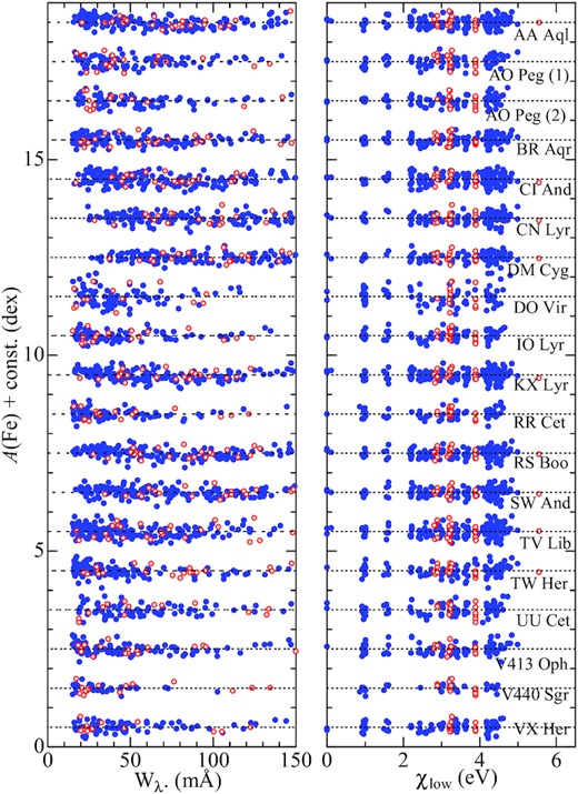
Fe abundance versus equivalent width relation (left-hand panel) and Fe abundance versus lower excitation potential relation (right-hand panel) corresponding to the finally established atmospheric parameters of Teff, log g, and vt for each of the 19 spectra of 18 RR Lyr stars (which were not used in Paper I and newly analysed in this study). The filled and open circles correspond to Fe i and Fe ii lines, respectively. The results for each stars are shown relative to the mean abundances indicated by the horizontal dashed lines, and vertically offset by 1.0 relative to the adjacent ones. (This figure is arranged in the same manner as in fig. 3 of Paper I, where the results for the other 15 spectra of 4 stars are depicted.)
In this connection, the parameters adopted in Paper II were determined (for 36 spectra of 23 stars) based on the same principle [requirements (i), (ii), and (iii)] but using a different computer programme (independently developed by the Chinese group) along with different set of Fe lines. These Paper II values of Teff, log g, vt, and [Fe/H] are compared with those of Paper I and those newly established for this study in Figs 2(a)–(d), where we can see that both are more or less consistent with each other except for a few cases (e.g. log g of DO Vir or vt of TW Her). An important difference is, however, that parameter determination for V445 Oph (somehow accomplished in Paper II) unfortunately failed in this study, because convergence could not be attained with anomalously large Fe abundances. Accordingly, V445 Oph (two spectra) had to be excluded from our analysis, which is the reason for the slight difference in the programme stars between this study (cf. Table 1) and Paper II (cf. table 1 therein).
![Comparison of the atmospheric parameters (and Na abundances) determined in Paper I and this study (abscissa) with those independently derived in Paper II (Liu et al. 2013) based on the same spectra (ordinate). (a) Teff, (b) log g, (c) vt, (d) [Fe/H], and (e) [Na/Fe] (note that Liu et al.’s Na abundances were derived based on the assumption of LTE, while non-LTE corrections are taken into consideration in this study).](https://oup.silverchair-cdn.com/oup/backfile/Content_public/Journal/mnras/514/2/10.1093_mnras_stac1431/1/m_stac1431fig2.jpeg?Expires=1750308268&Signature=KWtgWoVn8uAWq~df4wTVF0FSUraIRgfg2oAiEv-FRsMPcWYWDAO2Xe6Lvoi5gXVjEm7mIgEAE5OlO6edj6hTwztQUny51FvVmBahgcmBLH4OeRsGNwf2z~lT7HMVpRT--OYOi1QicFVaz1M9BsN4R05N07TvLE8JqiD~YYMDrTYTEW4YpQA9LMllpYa0-lHQlxHnYbXE6bdLzfyf1BES9uiPYxT4a8ttn1ATBeVvDSQyOO2lfueo6KbcmNKGGeTZmS1Ptbh4X3MqMRgSSg~6F60Ndy2PFLpM9eAu4~JFekdsDNhy1XjaXAy~vrBnaHk5VkCNrwNAWFhEITHhNb1I~Q__&Key-Pair-Id=APKAIE5G5CRDK6RD3PGA)
Comparison of the atmospheric parameters (and Na abundances) determined in Paper I and this study (abscissa) with those independently derived in Paper II (Liu et al. 2013) based on the same spectra (ordinate). (a) Teff, (b) log g, (c) vt, (d) [Fe/H], and (e) [Na/Fe] (note that Liu et al.’s Na abundances were derived based on the assumption of LTE, while non-LTE corrections are taken into consideration in this study).
The model atmosphere for each star (spectrum) was then constructed by three-dimensionally interpolating Kurucz’s (1993) ATLAS9 model grid (for vt = 2 km s−1) in terms of Teff, log g, and [Fe/H]. The non-LTE departure coefficients for C, N, O, and Na were also computed for a grid of 144 models resulting from combinations of six Teff values (5500, 6000, 6500, 7000, 7500, and 8000 K), four log g values (1.5, 2.0, 2,5, and 3.0), and six [Fe/H] values (−2.0, −1.5, −1.0, −0.5, 0.0, and + 0.5), which were further interpolated for each star as done for model atmospheres. Regarding more details about non-LTE calculations, see Takeda & Honda (2005) (for C, N, and O) and Takeda et al. (2003) (for Na) and the references therein.
4 ABUNDANCE DETERMINATION
In the differential analysis (relative to the Sun) adopted in this study, only one specific line feature of high quality (e.g. almost free from blending of other lines, unaffected by any telluric lines) is used for determining the abundance of each element: C i 5380 line (for C), N i 7468 line (for N), O i 7771/7774/7775 triplet lines (for O), and Na i 5682/5688 doublet lines (for Na). The determination procedures of abundances and related quantities (e.g. non-LTE correction, uncertainties due to ambiguities of atmospheric parameters) consist of two consecutive steps.
4.1 Synthetic spectrum fitting
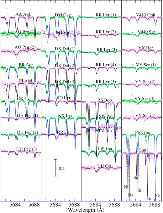
The first step is to find the solutions for the non-LTE abundances of relevant elements (|$A_{1}^{\rm N}, A_{2}^{\rm N}, \ldots$|), macrobroadening velocity (vM),3 and radial velocity (Vrad) such as those accomplishing the best fit (minimizing O − C residuals) between theoretical and observed spectra, while applying the automatic fitting algorithm (Takeda 1995). Four wavelength regions were selected for this purpose: (1) 5378–5382 Å region (for C), (2) 7460–7470 Å region (for N), (3) 7770–7777 Å region (for O), and 5681–5689.5 Å region (for Na). More information about this fitting analysis (varied elemental abundances, used data of atomic lines, etc.) is summarised in Table 2, and the atomic data of important lines are presented in Table 3. How the theoretical spectrum for the converged solutions fits well with the observed spectrum is displayed in Figs 3–6 for each region.
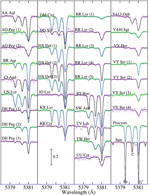
Synthetic spectrum fitting in the 5378–5382 Å region comprising the C i 5380 line. The best-fitting theoretical spectra are shown by solid lines. The observed data are plotted by symbols, where those used in the fitting are coloured in pink or green, while those rejected in the fitting (e.g. due to spectrum defect) are depicted in grey. In each panel, the spectra are arranged in the same order as in Table 1, and a vertical offset of 0.2 is applied to each spectrum relative to the adjacent one.
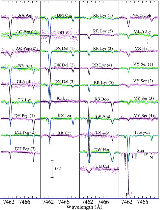
Synthetic spectrum fitting in the 7460–7470 Å region comprising the N i 7468 line. Otherwise, the same as in Fig. 3.
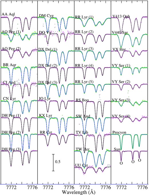
Synthetic spectrum fitting in the 7770–7777 Å region comprising the O i 7771/7774/7775 lines. A vertical offset of 0.5 is applied to each spectrum relative to the adjacent one. Otherwise, the same as in Fig. 3.
Synthetic spectrum fitting in the 5681–5689.5 Å region comprising the Na i 5682/5688 lines. Otherwise, the same as in Fig. 3.
Outline of spectrum-fitting analysis in this study.
| Purpose | Fitting range (Å) | Abundances varieda | Atomic data source | Figure |
|---|---|---|---|---|
| C abundance from C i 5380 | 5378–5382 | C, Ti, Fe | KB95m1 | Fig. 3 |
| N abundance from N i 7468 | 7460–7470 | N, Fe | KB95m2 | Fig. 4 |
| O abundance from O i 7771–5 | 7770–7777 | O | KB95m3 | Fig. 5 |
| Na abundance from Na i 5682/5688 | 5681–5689.5 | Na, Si, Sc, Fe, Ni | KB95 | Fig. 6 |
Notes. aThe abundances of other elements than these were fixed in the fitting.
KB95m1 – All the atomic line data presented in Kurucz & Bell (1995) were used, excepting that Ti ii 5379.15 and Fe i 5382.47 were neglected (by drastically suppressing their gf values to a negligible level).
KB95m2 – All the atomic line data were taken from Kurucz & Bell (1995), excepting that S i 7468.59 was neglected.
KB95m3 – All the atomic line data presented in Kurucz & Bell (1995) were used, excepting that the log gf values of four Fe i lines (at 7770.28, 7771.43, 7772.60, and 7774.00 Å) were empirically adjusted (as −5.12, −2.48, −2.16, and −2.27, respectively) while four lines (Ca i 7771.24, 7775.50, 7775.76, and Ti i 7773.90) were neglected (cf. section 3.3 in Takeda, Kawanomoto & Sadakane 1998).
KB95 – All the atomic line data given in Kurucz & Bell (1995) were used unchanged.
Adopted atomic data of the relevant C, N, O, and Na lines.
| Line | Multiplet | λ | χlow | log gf | Gammar | Gammas | Gammaw |
|---|---|---|---|---|---|---|---|
| No. | (Å) | (eV) | (dex) | (dex) | (dex) | (dex) | |
| C i 5380 | (11) | 5380.337 | 7.685 | −1.842 | (7.89) | −4.66 | (−7.36) |
| N i 7468 | (3) | 7468.312 | 10.336 | −0.270 | 8.64 | −5.40 | (−7.60) |
| O i 7771 | (1) | 7771.944 | 9.146 | +0.324 | 7.52 | −5.55 | (−7.65) |
| O i 7774 | (1) | 7774.166 | 9.146 | +0.174 | 7.52 | −5.55 | (−7.65) |
| O i 7775 | (1) | 7775.388 | 9.146 | −0.046 | 7.52 | −5.55 | (−7.65) |
| Na i 5682 | (6) | 5682.633 | 2.102 | −0.700 | (7.84) | (−5.00) | (−7.23) |
| Na i 5688 | (6) | 5688.204 | 2.104 | −0.404 | (7.84) | (−5.00) | (−7.23) |
Notes. Following the multiplet number, laboratory (air) wavelength, lower excitation potential, and gf value in columns 2–5, three kinds of damping parameters are presented in columns 6–8: Gammar is the radiation damping width (s−1) [log γrad], Gammas is the Stark damping width (s−1) per electron density (cm−3) at 104 K [log (γe/Ne)], and Gammaw is the van der Waals damping width (s−1) per hydrogen density (cm−3) at 104 K [log (γw/NH)].
All the data were taken from Kurucz & Bell (1995), except for the parenthesised damping parameters (unavailable in their compilation), for which the default values computed by the WIDTH9 programme were assigned.
4.2 Abundances from equivalent widths
As the second step, with the help of Kurucz’s (1993) WIDTH9 programme (which had been considerably modified in various respects; e.g. inclusion of non-LTE effects, treatment of total equivalent width for multicomponent lines; etc.), the equivalent widths (W) of the representative lines were ‘inversely’ computed from the abundance solutions (resulting from spectrum synthesis) along with the adopted atmospheric model/parameters; i.e. W5380 (for C i 5380), W7468 (for N i 7468), W7771 (for O i 7771), and W5688 (for Na i 5688), because they are easier to handle in practice (e.g. for estimating uncertainties due to errors in atmospheric parameters). Such derived W values were then analysed by using WIDTH9 to determine AN (NLTE abundance) and AL (LTE abundance), from which the NLTE correction Δ(≡ AN − AL) was further derived. Since the Sun is adopted as the standard star of abundance reference, the relative abundance is defined as [X/H] ≡|$A_{*}^{\rm N}$|(X) − |${\rm A}_{\odot }^{\rm N}$|(X), from which the X-to-Fe ratio is derived as [X/Fe] ≡ [X/H] − [Fe/H] (X = C, N, O, and Na). The resulting [C/Fe], [N/Fe], [O/Fe], and [Na/Fe] for each star are given in Table 1 (more complete results including W and Δ are separately presented in ‘abunds.dat’ of the supplementary material). Figs 7(C), 8(N), 9(O), and 10(Na) graphically show the equivalent width (W), non-LTE correction (Δ), non-LTE abundance (AN), and abundance variations in response to parameter changes (see the following Section 4.3), as functions of Teff.
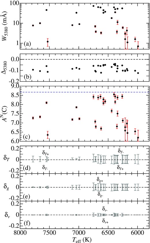
Carbon abundance and C i 5380-related quantities plotted against Teff. (a) W5380 (equivalent width of C i 5380, where the error bars attached to each symbol denote ±δW; cf. Section 4.3), (b) Δ5380 (non-LTE correction for C i 5380), (c) AN(C) (non-LTE abundance derived from C i 5380) where the error bar denotes ±δA defined in Section 4.3, (d) δT + and δT − (abundance variations in response to Teff changes of + 200 K and −200 K), (e) δg + and δg − (abundance variations in response to log g changes by +0.2 dex and −0.2 dex), and (f) δv + and δv − (abundance variations in response to perturbing the vt value by +20 per cent and −20 per cent). The solar |${\rm A}^{\rm N}_{\odot }$|(C) value of 8.67, which is adopted as the reference, is indicated by the horizontal dashed line in panel (c). Note that the ordinate in panel (a) is expressed in the logarithmic scale.
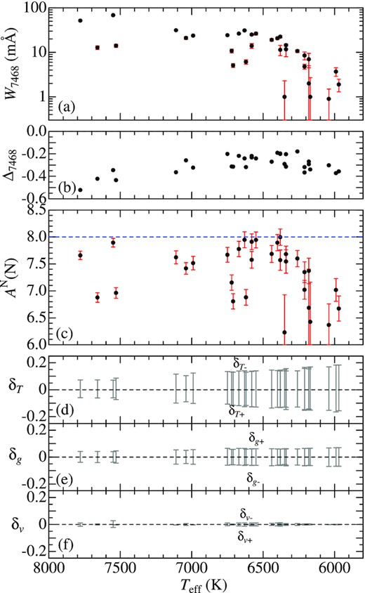
Nitrogen abundance and N i 7468-related quantities plotted against Teff. The reference solar |${\rm A}^{\rm N}_{\odot }$|(N) value of 8.00 is indicated by the horizontal dashed line in panel (c). Otherwise, the same as in Fig. 7.
4.3 Error estimation
In order to evaluate abundance errors caused by uncertainties in atmospheric parameters, we estimated six kinds of abundance variations (δT +, δT −, δg +, δg −, δv +, and δv −) for AN by repeating the analysis on the W values while perturbing the standard atmospheric parameters interchangeably by ±200 K in Teff, ±0.2 dex in log g, and |$\pm 20\,{\rm{per\,cent}}$| in vt (which are tentatively assigned as typical ambiguities of the parameters according to the results in Paper I). These δT ±, δg ±, and δv ± are plotted against Teff in panels (d), (e), and (f) of Figs 7–10. It can be seen from these figures that δT ± is generally more important (|$\lesssim$| 0.1–0.2 dex) than δg ± (reflecting the high-excitation nature of the adopted lines), while δv ± is insignificant (mainly due to the weakness of lines) except for the case of O i 7771 line.
Further, errors due to random noises of the observed spectra were estimated from S/N-related uncertainties in the equivalent width (W) by invoking the relation derived by Cayrel (1988), δW ≃ 1.6(wδx)1/2ϵ, where δx is the pixel size (0.03–0.05 Å), w is the line width (for which λvM/c was tentatively assigned; where λ is line wavelength, vM is the macrobroadening velocity, and c is the velocity of light), and ϵ ≡ (S/N)−1 (S/N is the signal-to-noise ratio in the neighbourhood of the line). The resulting δW (from a few tenths mÅ to several mÅ) are considerably smaller than W and thus generally unimportant as seen from the size of error bars in panel (a) of Figs 7–10, though this error may be exceptionally significant for very weak line cases where δW and W are comparable.
Therefore, for the case where lines are not weak (W ≥ 20 mÅ), the abundance uncertainties (δA) were evaluated by considering only the ambiguities in Teff, log g, and vt as |$\delta A \equiv \delta _{Tgv} \equiv (\delta _{T}^{2} + \delta _{g}^{2} + \delta _{v}^{2})^{1/2}$|, where δT, δg, and δv are defined as δT ≡ (|δT +| + |δT −|)/2, δg ≡ (|δg +| + |δg −|)/2, and δv ≡ (|δv +| + |δv −|)/2, respectively. Meanwhile, for the weak line case (W < 20 mÅ; where A ∝ W), the contribution due to δW was added as |$\delta A \equiv [\delta _{Tgv}^{2} + (\delta ^{^{\prime }}_{W})^2]^{1/2}$|, where |$\delta ^{^{\prime }}_{W}$| is the mean of |log (1 ± δW/W)|. These ±δA are shown as the error bars in panel (c) of Figs 7–10. The values of S/N, δW, δA for each element and for each star are also given in ‘abunds.dat’ of the supplementary material.
For the five stars (AO Peg, DH Peg, DX Del, RR Lyr, and VY Ser), for which several spectra at different phases are available, mean 〈[X/Fe]〉 values were calculated by averaging with the weight proportional to W/δW (equivalent width of the relevant line divided by its error), while the mean 〈[Fe/H]〉 was evaluated all with the same weight. These mean results are given in the last five rows in Table 1. Generally, [X/Fe] data based on very weak lines satisfying the condition δW/W > 0.5 were regarded as unreliable. Besides, quantities (e.g. [C/N] ratio or mean 〈[X/Fe]〉) essentially based on such unreliable [X/Fe] (and mean [X/Fe] values for which the standard deviation is larger than 0.2 dex) were also judged to be trustless. These dubious data are parenthesised in Table 1.
5 DISCUSSION
5.1 Observed trends of C, N, O, and Na abundances
Let us first elucidate the characteristics of surface abundances resulting from the analysis. The values of [C/Fe], [O/Fe], [N/Fe], and [Na/Fe] determined for each RR Lyr star are plotted against [Fe/H] in Figs 11(a), (b), (c), and (d), respectively, where the corresponding relations of unevolved dwarfs (taken from various literature) are also shown for comparison. Whether and how the surface abundance of an element X (X = C, N, O, and Na) has suffered changes in the course of stellar evolution may be studied by comparing the trends of [X/Fe]RRLyr (circles) and [X/Fe]dwarfs (crosses) with each other. The following tendencies are read from these figures:
The [O/Fe] versus [Fe/H] trend for RR Lyr stars is essentially the same as that for dwarfs (Fig. 11b), indicating that the surface abundance of O is almost kept without being appreciably affected by mixing.
While [C/Fe]dwarfs is apt to be supersolar (>0) like α elements, [C/Fe]RRLyr tends to be negative with a decrease in [Fe/H] (Fig. 11a), which means an enhanced C deficiency in the surface of RR Lyr stars towards lower metallicity.
In contrast, while [N/Fe]dwarfs distribute around ∼0 without any clear dependence upon metallicity, [N/Fe]RRLyr progressively increases with a decrease in [Fe/H] (Fig. 11c). This suggests an enhanced enrichment of N in the surface of RR Lyr stars as [Fe/H] is lowered.
Regarding Na, the behaviours of [Na/Fe]RRLyr and [Na/Fe]dwarfs with a decrease in [Fe/H] are quite similar (slightly supersolar at first followed by a downturn into subsolar regime at [Fe/H] |$\lesssim -1$|) (Fig. 11d),4 which indicates that the primordial composition of Na is almost retained in the surface of RR Lyr stars (like the case of O).
5.2 Checking with theoretical predictions
We are now able to check the mechanism of internal mixing by comparing these observed abundance trends with the surface abundance changes predictable from theoretical stellar evolution calculations. In Fig. 12 are shown the expected surface abundance changes of C, N, O, and Na during the course of post-main-sequence evolution of low-mass stars (plotted against Teff) calculated by Lagarde et al (2012b) for 0.85M ⊙ (with z = 0.0001 and 0.002) and 1.0 M⊙ (with z = 0.0001, 0.002, 0.004, and 0.014), where the results for two different assumptions of internal mixing (standard treatment, non-standard treatment including rotational and thermohaline mixing) are presented. In addition, since we are primarily interested in the abundance changes at the horizontal-branch (or red clump) phase, the phase points at the maximum Teff after the He-flash are marked by filled circle at each panel, and the corresponding values of log [X/X0] are separately given in Table 4.
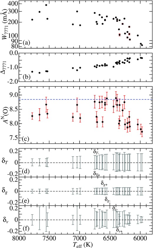
Oxygen abundance and O i 7771-related quantities plotted against Teff. The reference solar |${\rm A}^{\rm N}_{\odot }$|(O) value of 8.85 is indicated. Otherwise, the same as in Fig. 7.
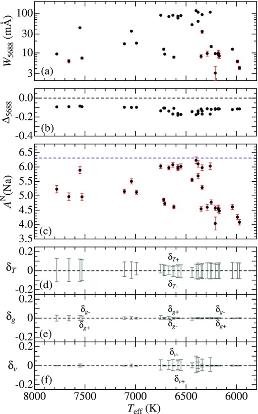
Sodium abundance and Na i 5688-related quantities plotted against Teff. The reference solar |${\rm A}^{\rm N}_{\odot }$|(Na) value of 6.31 is indicated by the horizontal dashed line in panel (c). Otherwise, the same as in Fig. 7.
![The final results of [C/Fe], [O/Fe], [N/Fe], [Na/Fe], and [C/N] derived in this study for RR Lyr stars (summarised in Table 1; mean values are used for AO Peg, DH Peg, DX Del, RR Lyr, and VY Ser) are plotted against [Fe/H] by blue circles in panels (a)–(e), respectively, while the relation between [Na/Fe] and [O/Fe] is depicted in panel (f). Note that open circles denote that these data are unreliable (i.e. parenthesised values in Table 1) and thus should not be seriously taken. In addition, the similar results for RR Lyr stars derived by Andrievsky et al. (2021) (for C, N, O; in panels a, b, c, and e) and those by Andrievsky et al. (2018) (for Na; in panels d and f) are shown by small red squares. The error bars of [C/N] shown in panel (e) denote $\pm \sqrt{\delta A_{\rm C}^{2}+\delta A_{\rm N}^{2}}$ (cf. Section 4.3 for the definition of δA). In panels (a)–(e), the results derived for other type of metal-poor stars taken from various literature are also overplotted by crosses for comparison: (a) Takeda & Honda’s (2005) non-LTE reanalysis results of [C/Fe] for dwarfs based on the C i 7771–9 and C i 9061–9111 data of Tomkin et al. (1992, 1995) and Akerman et al. (2004); (b) Takeda’s (2003) non-LTE reanalysis results of [O/Fe] for dwarfs (+subgiants) based on the O i 7771–5 data of Abia & Rebolo (1989) and Mishenina et al. (2000); (c) Laird’s (1985) [N/Fe] results for dwarfs (cf. his table 1); (d) Gehren et al.’s (2006) non-LTE [Na/Fe] results for dwarfs (cf. their table 2); (e) Afşar, Sneden & For’s ( 2012) [C/N] results for red horizontal-branch (RHB) candidates (which were calculated from CH-based [C/H] and O i based non-LTE [O/H] given in their table 7); here, only those stars which they clearly concluded to be RHB are coloured in pink (otherwise shown in grey inconspicuously). In addition, characteristic distribution regions of [C/N] theoretically expected for metal-poor giants under the influence of thermohaline mixing (roughly read from fig. 8 of Lagarde et al. 2019) are shown by green lines (long-dashed line indicates the sharp sequence corresponding to red clump stars, while the area embraced by short-dashed lines also represents the possible region of existence).](https://oup.silverchair-cdn.com/oup/backfile/Content_public/Journal/mnras/514/2/10.1093_mnras_stac1431/1/m_stac1431fig11.jpeg?Expires=1750308268&Signature=gaTBHyyqwWBQ2nvVFNWc9mAuH4tdW7DftxtbnAG04dpR6QdGLnV70GDTaWOBE~XUGUgkY3lJ9-0DUlsZ2FacLMlYFg5DnoQKcbb-o93XaCbiVSkUNJRWedfw9V5JSrCCc5wKu~usb~ZyaQ~EEgTZ0VdUEpblRCN0bFqlKhl71tDFL8eC9HVglI5~hCazcg~jnEv9forh7AW34HjJTOdn6vhCZALvvuXJaU7mkotaEMomZ9AWHGbQPBeldjf-y0tDTcSxKgGmqciop16hgidaGg2oE7hvQfFA-Lal7oJiLvJp2IAzByr1oMgcRQyC8vITauMLo41K8G4fjTvlg2N34g__&Key-Pair-Id=APKAIE5G5CRDK6RD3PGA)
The final results of [C/Fe], [O/Fe], [N/Fe], [Na/Fe], and [C/N] derived in this study for RR Lyr stars (summarised in Table 1; mean values are used for AO Peg, DH Peg, DX Del, RR Lyr, and VY Ser) are plotted against [Fe/H] by blue circles in panels (a)–(e), respectively, while the relation between [Na/Fe] and [O/Fe] is depicted in panel (f). Note that open circles denote that these data are unreliable (i.e. parenthesised values in Table 1) and thus should not be seriously taken. In addition, the similar results for RR Lyr stars derived by Andrievsky et al. (2021) (for C, N, O; in panels a, b, c, and e) and those by Andrievsky et al. (2018) (for Na; in panels d and f) are shown by small red squares. The error bars of [C/N] shown in panel (e) denote |$\pm \sqrt{\delta A_{\rm C}^{2}+\delta A_{\rm N}^{2}}$| (cf. Section 4.3 for the definition of δA). In panels (a)–(e), the results derived for other type of metal-poor stars taken from various literature are also overplotted by crosses for comparison: (a) Takeda & Honda’s (2005) non-LTE reanalysis results of [C/Fe] for dwarfs based on the C i 7771–9 and C i 9061–9111 data of Tomkin et al. (1992, 1995) and Akerman et al. (2004); (b) Takeda’s (2003) non-LTE reanalysis results of [O/Fe] for dwarfs (+subgiants) based on the O i 7771–5 data of Abia & Rebolo (1989) and Mishenina et al. (2000); (c) Laird’s (1985) [N/Fe] results for dwarfs (cf. his table 1); (d) Gehren et al.’s (2006) non-LTE [Na/Fe] results for dwarfs (cf. their table 2); (e) Afşar, Sneden & For’s ( 2012) [C/N] results for red horizontal-branch (RHB) candidates (which were calculated from CH-based [C/H] and O i based non-LTE [O/H] given in their table 7); here, only those stars which they clearly concluded to be RHB are coloured in pink (otherwise shown in grey inconspicuously). In addition, characteristic distribution regions of [C/N] theoretically expected for metal-poor giants under the influence of thermohaline mixing (roughly read from fig. 8 of Lagarde et al. 2019) are shown by green lines (long-dashed line indicates the sharp sequence corresponding to red clump stars, while the area embraced by short-dashed lines also represents the possible region of existence).
![Run of log [X/X0] (logarithmic mass fraction ratio of the relevant element at the surface relative to the initial value) with Teff according to Lagarde et al.’s (2012b) theoretical stellar evolution calculations. Shown here are the results for M = 0.85 M⊙ (left set of panels in two columns labelled as ‘z0001’ and ‘z002’ corresponding to z = 0.0001 and 0.002, or [Fe/H] = −2.16 and −0.86) and M = 1.0 M⊙ (right set of panels in four columns labelled as ‘z0001’, ‘z002’, ‘z004’, and ‘z014’ corresponding to z = 0.0001, 0.002, 0.004, and 0.014 = solar metallicity, or [Fe/H] = −2.16, −0.86, −0.56, and 0.00). The panels in the 1st, 2nd, 3rd, and 4th row are the log [X/X0] versus Teff diagrams for C (= 12C + 13C + 14C ≃ 12C), N (= 14N) O (= 16O + 17O + 18O ≃ 16O), and Na (= 23Na), respectively, while those in the bottom row show the corresponding log L versus Teff relations (theoretical Hertzsprung–Russell diagrams). Here, the data are restricted only to those after the zero-age main sequence (while neglecting those of the pre-main sequence stage). Note that two kinds of curves are shown corresponding to different treatments of internal mixing; i.e. standard treatment (blue lines) and non-canonical treatment including rotational and thermohaline mixing (pink lines). The bullet points (filled circles) marked at each panel indicate the horizontal-branch (or red-clump) phase closely related to RR Lyr stars, which is defined as the point of maximum Teff after the He ignition (the corresponding log [X/X0] data are separately presented in Table 4).](https://oup.silverchair-cdn.com/oup/backfile/Content_public/Journal/mnras/514/2/10.1093_mnras_stac1431/1/m_stac1431fig12.jpeg?Expires=1750308268&Signature=Yj01o8fZF6nWzzikyOhidTFOPaBbtdx-~tOWcQnm5wIPP-ih7DekvEChYDugtt~dlqiWqRWANb9-6xCn8JL9gRnLuVDZ2Tui5ypQ7gYUgH4P78upwQRdDTxYwbnqhqeW7Bysp2JrIeqOhxJgQ23abOJk6JGjXIn7NNKQ~M68KGX1Maesb~qZDz7EkFi8U6fXqMMZqSWTr7i9jBqcAWF8GzDOvNG3fL34NHWPwAGejQeBxnrt5YTKhK-TDTPVsH-qLXfg3giHG~MT5kYghliurDcV2E3PJNxyHcUk80HlTPVAkal9Tx5-5kPYE1kMyuzURpF2p8fU~wMyDbPOxIYpVg__&Key-Pair-Id=APKAIE5G5CRDK6RD3PGA)
Run of log [X/X0] (logarithmic mass fraction ratio of the relevant element at the surface relative to the initial value) with Teff according to Lagarde et al.’s (2012b) theoretical stellar evolution calculations. Shown here are the results for M = 0.85 M⊙ (left set of panels in two columns labelled as ‘z0001’ and ‘z002’ corresponding to z = 0.0001 and 0.002, or [Fe/H] = −2.16 and −0.86) and M = 1.0 M⊙ (right set of panels in four columns labelled as ‘z0001’, ‘z002’, ‘z004’, and ‘z014’ corresponding to z = 0.0001, 0.002, 0.004, and 0.014 = solar metallicity, or [Fe/H] = −2.16, −0.86, −0.56, and 0.00). The panels in the 1st, 2nd, 3rd, and 4th row are the log [X/X0] versus Teff diagrams for C (= 12C + 13C + 14C ≃ 12C), N (= 14N) O (= 16O + 17O + 18O ≃ 16O), and Na (= 23Na), respectively, while those in the bottom row show the corresponding log L versus Teff relations (theoretical Hertzsprung–Russell diagrams). Here, the data are restricted only to those after the zero-age main sequence (while neglecting those of the pre-main sequence stage). Note that two kinds of curves are shown corresponding to different treatments of internal mixing; i.e. standard treatment (blue lines) and non-canonical treatment including rotational and thermohaline mixing (pink lines). The bullet points (filled circles) marked at each panel indicate the horizontal-branch (or red-clump) phase closely related to RR Lyr stars, which is defined as the point of maximum Teff after the He ignition (the corresponding log [X/X0] data are separately presented in Table 4).
Theoretically simulated surface abundance changes of C, N, O, and Na at the horizontal branch.
| M | z | log [X/X0]C | log [X/X0]N | log [X/X0]O | log [X/X0]Na |
|---|---|---|---|---|---|
| (M⊙) | (dex) | (dex) | (dex) | (dex) | |
| Standard mixing | |||||
| 0.85 | 0.0001 | −0.0074 | +0.0315 | 0.0000 | 0.0000 |
| 0.85 | 0.002 | −0.0216 | +0.0810 | 0.0000 | 0.0000 |
| 1.00 | 0.0001 | −0.0662 | +0.2004 | −0.0001 | 0.0000 |
| 1.00 | 0.002 | −0.0686 | +0.2054 | −0.0001 | +0.1585 |
| 1.00 | 0.004 | −0.0655 | +0.1988 | −0.0001 | 0.0000 |
| 1.00 | 0.014 | −0.0532 | +0.1697 | 0.0000 | 0.0000 |
| Non-canonical mixing | |||||
| 0.85 | 0.0001 | −0.7986 | +0.6548 | −0.0041 | +0.4264 |
| 0.85 | 0.002 | −0.4932 | +0.5804 | −0.0009 | +0.1058 |
| 1.00 | 0.0001 | −0.5667 | +0.6250 | −0.0132 | +0.3629 |
| 1.00 | 0.002 | −0.4360 | +0.5752 | −0.0089 | +0.1601 |
| 1.00 | 0.004 | −0.3023 | +0.4907 | −0.0013 | +0.0394 |
| 1.00 | 0.014 | −0.1474 | +0.3452 | −0.0005 | +0.0064 |
Note. Presented are the log [X/X0] values (logarithmic ratio of the surface abundance relative to the primordial abundance) at the horizontal-branch (or red-clump) phase of maximum Teff after the He ignition (marked by the filled circles in Fig. 12), taken from the simulations of Lagarde et al. (2012b). The first six rows and the last six rows correspond to the cases of standard and non-standard mixing, respectively. See also the caption of Fig. 12 for more details.
5.2.1 Carbon and nitrogen
First of all, our attention is paid to C and N, since their surface abundances serve as the most important key for clarifying the physical process of evolution-induced mixing. It is apparent from Fig. 12 and Table 4 that a deficiency of C (Figs 12a and b) and an enrichment of N (Figs 12c and d) are generally expected. However, a clear difference exists between the two mixing cases (standard mixing, non-standard mixing); i.e. these surface abundance anomalies of C and N are progressively enhanced with a decrease of metallicity in the latter case with thermohaline mixing (while such a metallicity dependence is not seen in the former case). Accordingly, the [C/N] ratio (mostly negative) is predicted to decrease as [Fe/H] is lowered in the latter case of non-canonical mixing, which is just Lagarde et al. (2019) showed in their fig. 8.
The observed trends of [C/Fe] and [N/Fe] described in Section 5.1 (Figs 11a and c) are obviously in favour of the simulation done by including the effect of thermohaline mixing. Actually, the [C/N] versus [Fe/H] relations derived for our sample of RR Lyr stars are reasonably consistent with the distributions predicted for the case of non-canonical mixing (taken from fig. 8 of Lagarde et al. 2019) as shown in Fig. 11(e). Accordingly, it may be concluded that (only the standard mixing is not sufficient but) thermohaline mixing should also be taken into account for evolved low-mass stars (especially at lower metallicity).
5.2.2 Oxygen
Regarding oxygen, stellar evolution calculations suggest that its surface abundance is hardly affected whichever mixing mechanism is assumed (Table 4, Figs 12e and f). Therefore, the observed fact that [O/Fe] versus [Fe/H] trends for RR Lyr stars and for unevolved dwarfs are practically the same (cf Section 5.1) does not contradict the theoretical expectation, though it is not informative for elucidating the physical process of dredge-up.
5.2.3 Sodium
We see a problem with this element. Figs 12 (g) and (h) suggest that, while Na abundances at the surface suffer little changes regardless of metallicity (at least up to the stage of horizontal branch) for the case of standard mixing,5 they are predicted to be conspicuously enriched at the low-metallicity regime in the case of non-canonical mixing in the sense that the anomaly is enhanced with a decrease in metallicity (cf. Table 4). A comparison of these theoretical predictions with the observed results described in Section 5.1 (primordial Na abundances are almost retained at the surface of RR Lyr stars without being affected by evolution-induced mixing) naturally indicates that the former case of standard mixing is preferable as long as Na is concerned. Consequently, implication from C and N (supporting the non-canonical mixing) and that from Na (in favour of standard mixing) are inconsistent with each other. This may suggest that Lagarde et al.’s (2012b) calculations would require some more appropriate improvements.
5.3 Comparison with previous studies
Finally, some comments may be in order regarding the results of past related investigations in comparison with the consequences of this study.
Regarding Andrievsky et al.’s (2021) study (similar to the present one) on the CNO abundances of RR Lyr stars, 2 of their 9 sample stars are in common: DH Peg (considerably metal-poor) and DX Del (near-solar metallicity). Their results of ([Fe/H], [C/Fe], [N/Fe], [O/Fe]) are (−1.40, −0.16, +1.21, +0.68) for DH Peg and (−0.12, −0.09, +0.00, +0.30) for DX Del Comparing these with our values given in Table 1 (−1.16, −0.28, +0.76, +0.54) for DH Peg and (−0.23, −0.04, −0.09, +0.10) for DX Del, both are reasonably consistent in most cases (differences are within |$\lesssim$| 0.1–0.2 dex). Only [N/Fe] for DH Peg is the exceptional case, where an appreciable discrepancy (∼ 0.4–0.5 dex) is seen. An inspection on their non-LTE corrections for the N i 7468 line (−0.18 for DH Peg and −0.15 for DX Del) in comparison with our 〈Δ7468〉 values (−0.43 for DH Peg and −0.21 for DX Del; 〈Δ7468〉 is the W7468-weighted mean of Δ7468) suggests that the discrepancy in [N/Fe] of DH Peg may (at least partially) be attributed to the difference in the applied non-LTE correction.6
In any event, despite the existence of such a partial inconsistency, the consequences of Andrievsky et al. (2021) and this investigation are generally in accord with each other. The [Fe/H]-dependent trends of [C/Fe], [N/Fe], and [O/Fe] shown in fig. 6 of their paper are consistent with our results (cf Figs 11a, c, and b). Accordingly, the resulting [C/N] versus [Fe/H] relation for RR Lyr stars (cf their fig. 8) is quite similar to that obtained here (cf. Fig. 11e). In Fig. 11(e) are also overplotted the [C/N] ratios derived by Afşar et al. (2012) for 76 stars (many are G-type giants and subgiants), where we can see that their [C/N] results for red horizontal-branch (RHB) stars are consistent with the trend revealed by RR Lyr stars at the meal-poor regime ([Fe/H] |$\lesssim -0.5$|). Accordingly, all these results support the decreasing tendency of [C/N] ratios towards lower metallicity for horizontal-branch stars (at the post red-giant phase), indicating the importance of thermohaline mixing in low-mass giants.
Turning to Na, we may invoke the work of Andrievsky et al. (2018), who studied the O and Na abundances of 20 field RR Lyr stars. The [Na/Fe] versus [Fe/H] relation derived by them (cf fig. 8 therein) is in satisfactory agreement with ours as shown in Fig. 11(d). The mutual consistency is also confirmed for the correlation between [Na/Fe] and [O/Fe] (Fig. 11f). This supports our argument that surface Na abundances of RR Lyr stars have suffered little changes during the course of past evolution, which suggested a necessity of further theoretical improvement because of the conflicting implications between C/N and Na (cf. Section 5.2.3).
6 SUMMARY AND CONCLUSION
According to recent theoretical simulations on how the nuclear-processed materials in the stellar interior are salvaged to the surface in the course of evolution, not only the standard mixing (due to deepening of convective zone) but also the thermohaline mixing can play a significant role for the case of low-mass stars (|$M \lesssim$| 1 M⊙) in the sense that its importance increases with a decrease of metallicity. This can be tested by examining the surface abundances of key elements (such as C, N, O, and Na; more or less affected by mixing of H-burning products) determined for evolved giant stars in a wide metallicity range.
In order to check this theoretical prediction, photospheric abundances of C, N, O, and Na were spectroscopically determined for 22 RR Lyr stars (low-mass horizontal-branch stars after He-ignition currently in the Cepheid-instability strip) based on their 34 snap-shot spectra obtained by High-Dispersion Spectrograph of the Subaru Telescope.
The atmospheric parameters (Teff, log g, vt, and [Fe/H]) for each star were determined from the spectrum itself based on the equivalent widths of Fe i and Fe ii lines, and the resulting metallicities of the sample stars are in the range of |$-1.8 \lesssim$| [Fe/H] |$\lesssim 0.0$|.
The C, N, O, and Na abundances were determined by applying the synthetic spectrum-fitting technique to the regions comprising C i 5380, N i 7468, O i 7771–5, and Na i 5682/5688 lines, while taking the non-LTE effect adequately into consideration.
Comparing the resulting abundances ([C/Fe], [N/Fe], [O/Fe], and [Na/Fe]) of RR Lyr stars with those of unevolved metal-poor dwarfs at the same metallicity, we were able to check whether and how the surface abundance of each element has suffered a change due to evolution-induced mixing, by which information on the physical process of mixing may be gained in comparison with theoretical simulations.
Regarding C and N, a characteristic trend was confirmed that C is deficient while N is enriched, and the extent of these peculiarities tending to increase with a decrease in [Fe/H]. Accordingly, the [C/N] abundance ratio progressively decreases with a lowering of metallicity from ∼0 ([Fe/H] ∼0) to ∼−1 ([Fe/H] ∼−1.5). This lends support to the theoretical prediction for the case of non-canonical mixing (including thermohaline mixing).
In contrast, the observed abundances of O as well as Na in RR Lyr stars were found to be almost the same as those of dwarfs, which means that the surface compositions of these two elements are almost retained without being affected by dredge-up of nuclear-processed products.
The inertness of O is reasonably understandable, which is anyhow theoretically expected for whichever case of standard or non-canonical mixing. Meanwhile, according to currently available simulations, surface Na abundance is predicted to be progressively more enriched towards lower metallicity for the case of non-canonical mixing, while it hardly suffers changes for the case of standard mixing. Therefore, the observed behaviour of Na is more consistent with the case of standard mixing (i.e. without thermohaline mixing).
Consequently, since implications from C/N (supporting non-canonical mixing) and Na (in favour of standard mixing) are rather contradictory, this presumably means that the current theory is not complete and still has room for further improvement. The results obtained in this investigation may hopefully serve as observational constraints towards further progress on the theoretical side.
SUPPORTING INFORMATION
onlinedata.tar.gz
Please note: Oxford University Press is not responsible for the content or functionality of any supporting materials supplied by the authors. Any queries (other than missing material) should be directed to the corresponding author for the article.
ACKNOWLEDGEMENTS
This investigation is based on the data collected at Subaru Telescope, which is operated by the National Astronomical Observatory of Japan. This research has made use of the SIMBAD data base, operated by CDS, Strasbourg, France.
DATA AVAILABILITY
The basic data and results underlying this article are presented as the online supplementary material. The original observational data are in the public domain and available at https://smoka.nao.ac.jp/index.jsp (SMOKA Science Archive site).
Footnotes
As usual, [X/H] is the differential abundance for element X of a star relative to the Sun defined as [X/H] ≡ A*(X) − A⊙(X), where A(X) is the logarithmic number abundance of element X (so normalized with respect to H as A(H) = 12.00). Likewise, the notation [X/Y] is defined as [X/Y] ≡ [X/H] − [Y/H].
Regarding the term ‘non-canonical mixing’, three kinds of mixing processes are generally involved (cf. Lagarde et al. 2012b): (i) convective (standard) mixing, (ii) thermohaline mixing, and (iii) rotational mixing. Among these, the last rotational one may be regarded as insignificant in low-mass (|$M \lesssim$| 1 M⊙) stars of our concern, because efficient rotational braking (loss of angular momentum) would take place when they are on the main sequence (late-type dwarfs). Accordingly, when non-canonical mixing is referred to in the remainder of this paper, we do not explicitly mention about rotational mixing but confine only to thermohaline mixing (e.g. the term ‘thermohaline mixing’ is occasionally used to mean the equivalent concept of ‘non-canonical mixing’ for simplicity). In Lagarde et al.’s (2019) population-synthesis calculations for [C/N] where comparatively lower-mass stars are primarily concerned, the effect of rotation is not included in the non-standard mixing (regarding the impact of rotational mixing, see the other papers of the same group; e.g. Charbonnel & Lagarde 2010; Lagarde et al. 2012a).
This vM is the e-folding half width of the Gaussian macrobroadening function to be convolved, fM(v) ∝ exp [ − (v/vM)2], which represents the combined effects of rotational broadening, macroturbulence, and instrumental broadening.
Note that generally higher [Na/Fe] values were obtained in Paper II (cf. fig. 5 therein) in comparison with those of this study. This systematic discrepancy (cf. fig. 2e) is attributed to that fact that the non-LTE effect was not taken into account in the analysis of Paper II.
As shown in Table 4, an appreciable increase of surface Na by + 0.16 dex is seen even in the standard mixing only for the case of M = 1 M⊙ and z = 0.002 (its change appears to begin already at the first dredge-up phase before He ignition), in contrast to other (M, z) combinations where the primordial Na is retained in the standard mixing case. Considering a possibility that this might be due to some kind of error, we refrain from taking into account this data for the time being.
Andrievsky et al. (2021) reanalysed Takeda & Sadakane’s (1997) equivalent width data of CNO lines for the metal-poor ([Fe/H] ∼−1.5) horizontal-branch star HD 161817. As seen from tables 5 and 6 of their paper, their |Δ| values for the N i 8683/8686/8706 lines are generally smaller than those of Takeda & Sadakane (1997), just like the case for Δ7468 of DH Peg described here. Besides, they reported that their LTE abundances are also in disagreement. Since N abundance determinations from these N i 8683/8686/8706 lines are severely affected by the strong wings of Paschen lines, the way how the background opacity of these overlapping H i lines may have been different between Takeda & Sadakane (1997) and Andrievsky et al. (2021).
