


ABSTRACT
We present the results from a high-cadence, multiwavelength observation campaign of AT 2016jbu (aka Gaia16cfr), an interacting transient. This data set complements the current literature by adding higher cadence as well as extended coverage of the light-curve evolution and late-time spectroscopic evolution. Photometric coverage reveals that AT 2016jbu underwent significant photometric variability followed by two luminous events, the latter of which reached an absolute magnitude of MV ∼ −18.5 mag. This is similar to the transient SN 2009ip whose nature is still debated. Spectra are dominated by narrow emission lines and show a blue continuum during the peak of the second event. AT 2016jbu shows signatures of a complex, non-homogeneous circumstellar material (CSM). We see slowly evolving asymmetric hydrogen line profiles, with velocities of 500 km s−1 seen in narrow emission features from a slow-moving CSM, and up to 10 000 km s−1 seen in broad absorption from some high-velocity material. Late-time spectra (∼+1 yr) show a lack of forbidden emission lines expected from a core-collapse supernova and are dominated by strong emission from H, He i, and Ca ii. Strong asymmetric emission features, a bumpy light curve, and continually evolving spectra suggest an inhibit nebular phase. We compare the evolution of H α among SN 2009ip-like transients and find possible evidence for orientation angle effects. The light-curve evolution of AT 2016jbu suggests similar, but not identical, circumstellar environments to other SN 2009ip-like transients.
1 INTRODUCTION
Massive stars that eventually undergo core-collapse when surrounded by some dense circumstellar material (CSM) are known as Type IIn supernovae (SNe) (Schlegel 1990; Filippenko 1997; Fraser 2020). This is signified in spectra by a bright, blue continuum with narrow H and He i emission lines at early times. Type IIn SNe spectra show narrow (∼100–500 km s−1) components arising in the photoionized, slow-moving CSM. Intermediate-width emission lines (∼1000 km s−1) arise from either electron scattering of photons in narrower lines or emission from gas shocked by SN ejecta. Some events also show very broad emission or absorption features (∼10 000 km s−1) arising from fast ejecta, typically associated with material ejected in a core-collapse explosion.
The existence of the dense CSM indicates that the Type IIn progenitors have high mass-loss rates shortly before their terminal explosion. This dense material at the end of a star’s life can come from several pathways (see reviews by Puls, Vink & Najarro 2008; Smith 2014; Fraser 2020, for further detail.)
Complicating this picture are a growing number of extragalactic transients that show narrow emission lines in their spectra (indicating CSM) but have much fainter absolute magnitudes than most typical Type IIn SNe. These events are often termed SN Impostors (Van Dyk et al. 2000; Maund et al. 2006; Pastorello & Fraser 2019), and are believed in many cases to be extragalactic Luminous Blue Variables (LBVs) experiencing giant eruptions (e.g. SN 2000ch; Wagner et al. 2004; Pastorello et al. 2010). These eruptions do not completely destroy their progenitors.
Perhaps the best studied exemplar of the confusion between LBVs, SN impostors, and genuine Type IIn SNe is SN 2009ip. SN 2009ip was found on 2009 August 26 at ∼17.9 mag in NGC 7259 by CHASE project team members (Maza et al. 2009). This transient was originally classified as a Type IIn SN, and then reclassed as an impostor when it became clear that the progenitor had survived. SN 2009ip was characterized by a year-long phase of erratic variability that ended with two luminous outbursts a few weeks apart in 2012 (Li et al. 2009; Drake et al. 2010; Margutti et al. 2012; Fraser et al. 2013; Pastorello et al. 2013; Graham et al. 2014; Smith, Mauerhan & Prieto 2014).
From pre-explosion images taken 10 yr prior to the 2009 discovery, the progenitor star of SN 2009ip was suggested to be an LBV with a mass of 50–80 M⊙ (Smith et al. 2010; Foley et al. 2011). There is much debate on the fate of SN 2009ip. Some argue that SN 2009ip has finally exploded as a genuine Type IIn SN during the 2012 outburst (Mauerhan et al. 2013; Prieto et al. 2013). However, other authors remain agnostic as to SN 2009ip’s fate as a Core Collpase Supernova (CCSN), pointing to the absence of any evidence for nucleosynthesized material in late-time spectra, as well as SN 2009ip not fading significantly below the progenitor magnitude (Fraser et al. 2013, 2015; Margutti et al. 2014). Since the discovery of SN 2009ip, a number of remarkably similar transients have been found. The growing family of SN 2009ip-like transients share similar spectral and photometric evolution. SN 2009ip-like transients have the following observable traits.
History of variability lasting (at least) ∼10 yr with outbursts reaching Mr ∼ −11 ± 3 mag.
Two bright luminous events with the first peak reaching a magnitude of Mr ∼ −13 ± 2 mag followed by the second peak reaching Mr ∼ −18 ± 1 mag several weeks later.
Spectroscopically similar to a Type IIn SN i.e. narrow emission features and a blue continuum at early times.
Restrictive upper limits to the mass of any explosively synthesized 56Ni.
In this paper, we focus on one such SN 2009ip-like transient. AT 2016jbu (also known as Gaia16cfr; Bose et al. 2017) was discovered at RA = 07:36:25.96, Dec. = −69:32:55.25 (J2000) by the Gaia satellite on 2016 December 1 with a magnitude of G = 19.63 (corresponding to an absolute magnitude of −11.97 mag for our adopted distance modulus). The Public ESO Spectroscopic Survey for Transient Objects (PESSTO) collaboration (Smartt et al. 2015) classified AT 2016jbu as an SN 2009ip-like transient due to its spectral appearance and apparent slow rise (Fraser et al. 2017). Fraser et al. (2017) also find that the progenitor of AT 2016jbu seen in archival Hubble Space Telescope (HST) images is consistent with a massive (<30 M⊙) progenitor. The transient was independently discovered by B. Monard in late December who reported the likely association of AT 2016jbu to its host, NGC 2442. AT 2016jbu is situated to the south of NGC 2442, a spiral galaxy commonly referred to as the Meathook galaxy. NGC 2442 has hosted two other SNe including SN 1999ga, a low-luminosity Type II SN (Pastorello et al. 2009) and SN 2015F, a Type Ia SN (Cartier et al. 2017). We mark their respective locations in Fig. 1. Bose et al. (2017) and Prentice et al. (2018) reported initial spectroscopic observations and classification of AT 2016jbu.
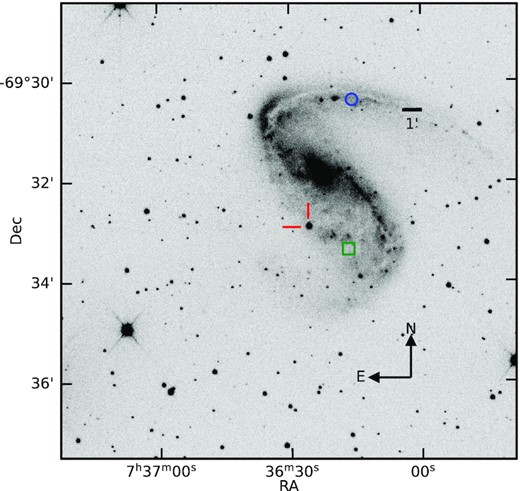
Finder chart for AT 2016jbu. The image is a 60s r-band exposure taken with the LCO 1-m. AT 2016jbu is situated to the south-east of the spiral galaxy NGC 2442 nucleus and is indicated with a red cross reticle in the centre of the image. This location lies on the outskirts of a Superbubble (Pancoast et al. 2010), with a high star formation rate. We also include the location of the Type Ia SN 2015F (blue circle, north-west of image centre; Cartier et al. 2017) and the Type II SN 1999ga (green square, south-west of image centre; Pastorello et al. 2009).
AT 2016jbu has been previously studied by Kilpatrick et al. (2018) (hereafter referred to as K18). K18 find that AT 2016jbu appears similar to a Type IIn SN, with narrow emission lines and a blue continuum. The Gaia light curve shows that AT 2016jbu has a double-peaked light curve showing two distinct events (we refer to these events as Event A and Event B). This is common in SN 2009ip-like transient with Event B reaching an absolute magnitude of r ∼ −18 mag. H α displays a double-peaked profile a few weeks after maximum brightness, indicating a complex CSM environment. K18 model H α using a multicomponent line profile including a shifted blue emission feature that grows with time, with their final profile similar to that of the Type IIn SN 2015bh (Elias-Rosa et al. 2016; Thöne et al. 2017) at late times.
Using HST images, spanning 10 yr prior to the 2016 transient, K18 report that AT 2016jbu underwent a series of outbursts in the decade prior, similar to SN 2009ip, and find the progenitor is consistent with a ∼18 M⊙ progenitor star, with strong evidence of reddening by circumstellar (CS) dust (which would allow for a higher mass). Performing dust modelling using Spitzer photometry, K18 find the spectral energy distribution (SED) ∼10 yr prior is fitted well with a warm dust shell at 120 au. They find that, given typical CSM velocities, it is unlikely that this dusty shell is in the immediate vicinity of the progenitor and is unlikely to be seen during the 2016 event. This means that the progenitor of AT 2016jbu was experiencing episodic mass-loss within years to decades of its most recent explosion.
This paper focuses on photometry and spectra obtained for AT 2016jbu which is not covered by K18. In particular, this includes searching through historic observations of AT 2016jbu’s host, NGC 2442 for signs of variability, as is expected for SN 2009ip-like transients, as well as presenting high-cadence data for Event A and the late-time photometric and spectroscopic evolution.
We take the distance modulus for NGC 2442 to be 31.60 ± 0.06 mag, which is a weighted average of the values determined from HST observations of Cepheids (|$\mu =31.511\pm 0.053~\mathrm{ mag}~$|; Riess et al. 2016) and from the SN Ia 2015F (|$\mu =31.64\pm 0.14$| mag; Cartier et al. 2017). This corresponds to a metric distance of 20.9 ± 0.58 Mpc. We adopt a redshift of z = 0.00489 from H i Parkes All-Sky Survey (Wong et al. 2006). The foreground extinction towards NGC 2442 is taken to be AV = 0.556 mag, from Schlafly & Finkbeiner (2011) via the NASA Extragalactic Database (NED1). We correct for foreground extinction using RV = 3.1 and the extinction law given by Cardelli, Clayton & Mathis (1989). We do not correct for any possible host galaxy or CS extinction, however we note that the blue colours seen in the spectra of AT 2016jbu do not point towards significant reddening by dust. We take the V-band maximum during the second, more luminous event in the light curve (as determined through a polynomial fit) as our reference epoch (MJD 57784.4 ± 0.5; 2017 January 31).
This is the first of two papers discussing AT 2016jbu. In this paper (Paper I), we report spectroscopic and photometric observations of AT 2016jbu. In Section 2, we present details of data reduction and calibration. In Section 3 and Section 4 we discuss the photometric and spectroscopic evolution of AT 2016jbu, respectively. In Section 5, we compare AT 2016jbu to SN 2009ip-like transients, and also consider the observational evidence for core-collapse.
Brennan et al. (2021) (hereafter Paper II) focus on the progenitor of AT 2016jbu, its environment, and using modelling to constrain the physical properties of this event.
2 OBSERVATIONAL DATA
The optical light-curve evolution of AT 2016jbu has been previously discussed in K18. Their analysis covers Event B up to ∼+140 d past maximum brightness. We present a higher cadence photometric data set that covers both Event A, Event B, and late-time observations up to ∼+ 575 d. This high-cadence data set allows for a more detailed photometric analysis of AT 2016jbu, which will be discussed in Section 5. K18 discuss the spectral evolution of AT 2016jbu from −27 d until + 118 d. Our observational campaign presented here contains increased converge during this period as well as observations up until +420 d allowing for late-time spectral follow-up.
2.1 Optical imaging and reduction
Optical imaging of AT 2016jbu in BVRri filters was obtained with the 3.58m ESO New Technology Telescope (NTT) + EFOSC2, as part of the ePESSTO survey. All images were reduced in the standard fashion using the PESSTO pipeline (Smartt et al. 2015); in brief images were bias and overscan subtracted, flat fielded, before being cleaned of cosmic rays using a Laplacian filter (van Dokkum 2001). Further optical imaging was obtained from the Las Cumbres Observatory network of robotic 1-m telescopes as part of the Global Supernova Project. These data were reduced automatically by the banzai pipeline, which runs on all Las Cumbres Observatory (LCO) Global Telescope images (Brown et al. 2013). Images were also obtained from the Watcher telescope. Watcher is a 40 cm robotic telescope located at Boyden Observatory in South Africa (French et al. 2004). It is equipped with an Andor IXon EMCCD camera providing a field of view of 8 × 8 arcmin. The Watcher data were reduced using a custom-made pipeline written in Python.
AT 2016jbu was monitored using the Gamma-Ray Burst Optical/Near-Infrared Detector (GROND; Greiner et al. (2008)), a seven-channel imager that collects multicolour photometry simultaneously with Sloan-griz and JHK/Ks bands, mounted at the 2.2 m MPG telescope at ESO La Silla Observatory in Chile. The images were reduced with the GROND pipeline (Krühler et al. 2008), which applies de-bias and flat-field corrections, stacks images, and provides astrometry calibration. Due to the bright host galaxy we disabled line-by-line fitting of the sky subtraction for the GROND NIR data since this caused oversubtraction artefacts. Since the photometry background estimation is limited by the extended structure of the host galaxy and not by the large-scale variation in the background of the image, we do not expect any adverse effects from this change.
Unfiltered imaging of AT 2016jbu was also obtained by B. Monard. Observations of AT 2016jbu were taken at the Kleinkaroo Observatory (KKO), Calitzdorp (Western Cape, South Africa) using a 30 cm telescope Meade RCX400 f/8 and CCD camera SBIG ST8-XME in 2 × 2 binned mode. Unfiltered images were taken with 30 s exposures, dark subtracted and flat fielded and calibrated against r-band sequence stars. Nightly images resulted from stacking (typically five to eight) individual images.
We also recovered a number of archival images covering the site of AT 2016jbu. Two epochs of g and r imaging from the Dark Energy Camera (DECam) (Flaugher et al. 2015) mounted on the 4 m Blanco Telescope at the Cerro Tololo Inter-American Observatory (CTIO) were obtained from the NOIRLab Astro Data Archive. The science-ready reduced ‘InstCal’ images were used in our analysis. In addition to these, we downloaded deep imaging taken in 2005 with the MOSAIC-II imager (the previous camera on the 4 m Blanco Telescope). As for the DECam data, the ‘InstCal’ reductions of MOSAIC-II images were used. We note that the filters used for the MOSAIC-II images (Harris V and R, Washington C Harris & Canterna 1979) are different from the rest of our archival data set. The Harris filters were calibrated to Johnson-Cousins V and R. The Washington C filter data are more problematic, as this bandpass lies between Johnson-Cousins U and B. We calibrated our photometry to the latter, but this should be interpreted with appropriate caution.
Deep Very Large Telescope (VLT) + OmegaCAM images taken with i, g, and r filters in 2013, 2014, and 2015, respectively, were downloaded from the ESO archive. The Wide Field Imager (WFI) mounted on the 2.2-m MPG telescope at La Silla also observed NGC 2442 on a number of occasions between 1999 and 2010 in B, V, and R; these images are of particular interest as they are quite deep, and extend our monitoring of the progenitor as far back as −15 yr. Both the OmegaCAM and WFI data were reduced using standard procedures in iraf.2
NED contains a number of historical images of NGC 2442, dating back to 1978. We examined each of these but found none that contained a credible source at the position of AT 2016jbu.
Several transient surveys also provided photometric measurements for AT 2016jbu. Gaia G-band photometry for AT 2016jbu was downloaded from the Gaia Science Alerts web pages. As this photometry was taken with a broad filter that covers approximately V and R, we did not attempt to calibrate it on to the standard system. V-band imaging was also taken as part of the All-Sky Automated Survey for Supernovae (ASAS-SN Shappee et al. 2014; Kochanek et al. 2017).3
The OGLE IV Transient Detection System (Kozłowski et al. 2013; Wyrzykowski et al. 2014) also identified AT 2016jbu, and reported I-band photometry via the OGLE webpages.4
The Panchromatic Robotic Optical Monitoring and Polarimetry Telescopes (PROMPT) (Reichart et al. 2005) obtained imaging of AT 2016jbu in BVRI filters, and as discussed in Section 5.1.1, unfiltered PROMPT observations of NGC 2442 were also used to constrain the activity of the progenitor of AT 2016jbu over the preceding decade. Images were taken with the PROMPT1, PROMPT3, PROMPT4, PROMPT6, PROMPT7, and PROMPT8 robotic telescopes (all located at the CTIO). PROMPT4 and PROMPT6 have a diameter of 40 cm, while PROMPT1, PROMPT3, and PROMPT8 have a diameter of 60 cm and PROMPT7 has a diameter of 80 cm. All images collected with the PROMPT units were dark subtracted and flat-field corrected. In case multiple images were taken in consecutive exposures, the frames were registered and stacked to produce a single image.
NGC 2442 was also serendipitously observed with the FOcal Reducer/low dispersion Spectrograph 2 (FORS2) as part of the late-time follow-up campaign for SN 2015F (Cartier et al. 2017). Unfortunately, most of these data were taken with relatively long exposures, and AT 2016jbu was saturated. However, a number of pre-discovery images from the second half of 2016, as well as late-time images from 2018 are of use. These data were reduced (bias subtraction and flat fielding) using standard iraf tasks.
2.2 UV imaging
UV and optical imaging was obtained with the Neil Gehrels Swift Observatory (Swift) with the Ultra-Violet Optical Telescope (UVOT). The pipeline reduced data were downloaded from the Swift Data Center. The photometric reduction follows the same basic outline as Brown et al. (2009). In short, a 5 arcsec radius aperture is used to measure the counts for the coincidence loss correction, and a 3 arcsec source aperture (based on the error) was used for the aperture photometry and applying an aperture correction as appropriate [based on the average Point Spread Function (PSF) in the Swift HEASARC’s calibration database (CALDB) and zero-points from Breeveld et al. 2011].
Subsequent to the photometric reduction of our Swift data, there was an update to the Swift CALDB with time-dependant zero-points which we have not accounted for. Given that our Swift observations occurred in early 2017, this would amount to a |$\sim ~3{{\ \rm per\ cent}}$| shift in zero-point and would not lead to a significant change in our light curve.
2.3 NIR imaging
Near-infrared imaging was obtained with NTT + SOFI as part of the ePESSTO survey, and with GROND as mentioned previously. In both cases JHK/Ks filters were used. SOFI data were reduced using the PESSTO pipeline (Smartt et al. 2015). Data were corrected for flat-field and illumination, sky subtraction was performed using (in most instances) off-target dithers, before individual frames were co-added to make a science-ready image.
In addition to the follow-up data obtained for AT 2016jbu with SOFI, we examined pre-discovery SOFI images taken as part of the PESSTO follow-up campaign for SN 2015F. We downloaded reduced images from the ESO Phase 3 archive which covered the period up to 2014 April. Two subsequent epochs of SOFI imaging from 2016 October were taken after PESSTO SSDR3 was released, and so we downloaded the raw data from the ESO archive, and reduced these using the PESSTO pipeline as for the rest of the SOFI follow-up imaging.
Fortuitously, the ESO VISTA telescope equipped with VIRCAM observed NGC 2442 as part of the VISTA Hemisphere Survey (VHS) in 2016 December. We downloaded the reduced images as part of the ESO Phase 3 data release from VHS via ESO Science Portal. Photometry was performed using AutoPhOT, see Section 2.6.
2.4 MIR imaging
We queried the WISE data archive at the NASA/IPAC infrared science archive, and found that AT 2016jbu was observed in the course of the NEOWISE reactivation mission (Mainzer et al. 2014). As the spatial resolution of WISE is low compared to our other imaging, we were careful to select only sources that were spatially coincident with the position of AT 2016jbu. There were numerous detections of AT 2016jbu in the W1 and W2 bands over a 1 week period shortly before the maximum of Event B (MJD 57784.4 ± 0.5). The profile-fitted magnitudes measured for each single exposure (L1b frames) were averaged within a 1 d window.
We also examined the pre-explosion images covering the site of AT 2016jbu in the Spitzer archive, taken on 2003 November 21 (MJD 52964.1). Some faint and apparently spatially extended flux can be seen at the location of AT 2016jbuin Ch1, although there is a more point-like source present in Ch2. No point source is seen in Ch3 and Ch4. K18 report values of 0.0111 ± 0.0032 mJy and 0.0117 ± 0.0027 mJy in Ch1 and Ch2 (corresponding to magnitude of 18.61 mag and 17.917 mag, respectively) and similarly do not detect a source in Ch4 and Ch4 for the 2003 images.
2.5 X-ray imaging
A target of opportunity observation (ObsID: 0794580101) was obtained with XMM–Newton (Jansen et al. 2001) on 2017 January 26 (MJD 57779) for a duration of ∼57 ks. The data from EPIC-PN (Strüder et al. 2001) were analysed using the latest version of the Science Analysis Software, sas v185 including the most updated calibration files. The source and background were extracted from a 15 arcsec region avoiding a bright nearby source. Standard filtering and screening criteria were then applied to create the final products.
X-ray imaging was also taken with the XRT on board Swift. These observations are much less sensitive than the XMM–Newton data, and so we do not expect a detection. Using the online XRT analysis tools6 (Evans et al. 2007, 2009) we co-added all XRT images covering the site of AT 2016jbu available in the Swift data archive. No source was detected coincident with AT 2016jbu in the resulting ∼100 ks stacked image.
2.6 Photometry with the AutoPHoT pipeline
The data set presented in this paper for AT 2016jbu comprises ∼3000 separate images from around 20 different telescopes. To expedite photometry on such large and hetrogeneous data sets, we have developed a new photometric pipeline called AutoPhOT (AUTOmated PHotometry Of Transients; Brennan & Fraser 2022). AutoPhOT has been used to measure all photometry presented in this paper, with the exception of imaging from space telescopes (i.e. Swift, Gaia, WISE, Spitzer, XMM–Newton OM, and HST), as well as from ground-based surveys which have custom photometric pipelines (i.e. ASAS-SN and OGLE).
AutoPhOT7,8 is a Python3-based photometry pipeline built on a number of commonly used astronomy packages, mostly from astropy. AutoPhOT is able to handle hetrogeneous data from different telescopes, and performs all steps necessary to produce a science-ready light curve with minimal user interaction.
In brief, AutoPhOT will build a model for the PSF in an image from bright isolated sources in the field (if no suitable sources are present then AutoPhOT will fall back to aperture photometry). This PSF is then fitted to the transient to measure the instrumental magnitude. To calibrate the instrumental magnitude on to the standard system (either AB magnitudes for Sloan-like filters or Vega magnitudes for Johnson-Cousins filters) for this work on AT 2016jbu, the zero-point for each image is found from catalogued standards in the field. For griz filters, the zero-point was calculated from magnitudes of sources in the field taken from the SkyMapper Southern Survey (Onken et al. 2019). For Johnson-Cousins filters, we used the tertiary standards in NGC 2442 presented by Pastorello et al. (2009). In the case of the NIR data (JHK) we used sources taken from the Two Micron All-Sky Survey (2MASS; Skrutskie et al. 2006). There is no u-band photometry covering this portion of the sky. We use U-band photometry from Cartier et al. (2017) and convert to u-band using table 1 in Jester et al. (2005). We include Swope photometry from K18 in Fig. 2 to show that our u-band is consistent.
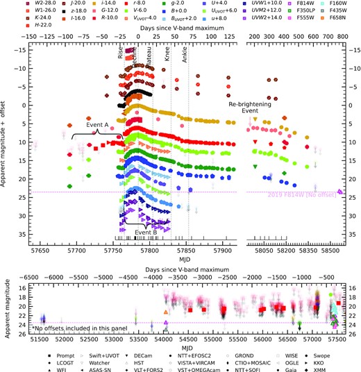
The complete multiband observed photometry for AT 2016jbu. The upper panel covers the period from the start of Event A (first detection at −91 d from VLT + FORS2) until the end of our monitoring campaign ∼2 yr after Event B peak. Offsets (listed in the legend) have been applied to each filter for clarity in the upper panels only. Note that there is a change in scale in the X-axis after 135 d. We indicate Event A and the rise and decline of the peak of Event B. Epochs where spectra were taken are marked with vertical ticks. We also include the published Swope photometry from K18 (given as filled circles) to demonstrate that our photometry is consistent. We include a horizontal magenta dotted line in all panels to demonstrate the early 2019 F814W magnitudes (Paper II). We only plot error bars greater than 0.1 mag. The lower panel shows detections and upper limits over a period from ∼18 yr prior to Event A. No offsets are included in this panel; light points with arrows show upper limits, while solid points are detections.
Log of optical, UV, and NIR spectra obtained for AT 2016jbu. MJD refers to the start of the exposure. Phase is with respect to the time of V-band maximum (MJD 57784.4 ± 0.5).
| Date | MJD | Phase (d) | Instrument | Grism |
|---|---|---|---|---|
| 2016-12-31 | 57753.0 | −31.4 | DuPont + WFCCD | Blue grism |
| 2017-01-02 | 57755.4 | −28.0 | Magellan + FIRE | LDPrism |
| 2017-01-04 | 57757.3 | −27.1 | NTT + EFOSC2 | Gr#13 |
| 2017-01-06 | 57759.3 | −25.1 | NTT + EFOSC2 | Gr#11 |
| 2017-01-08 | 57761.7 | −22.7 | FTS + FLOYDS | red/blue |
| 2017-01-15 | 57768.5 | −15.9 | FTS + FLOYDS | red/blue |
| 2017-01-17 | 57770.2 | −14.2 | NTT + EFOSC2 | Gr#11 + Gr#16 |
| 2017-01-18 | 57771.3 | −13.1 | NTT + EFOSC2 | Gr#11 + Gr#16 |
| 2017-01-20 | 57773.2 | −11.2 | NTT + EFOSC2 | Gr#11 |
| 2017-01-20 | 57773.1 | −10.7 | Gemini S + FLAMINGOS2 | JH |
| 2017-01-22 | 57775.2 | −9.2 | Swift + UVOT | UV Grism |
| 2017-01-26 | 57779.3 | −5.1 | NTT + EFOSC2 | Gr#11 + Gr#16 |
| 2017-01-27 | 57780.0 | −4.4 | ANU 2.3m + WiFeS | red/blue |
| 2017-01-27 | 57780.2 | −4.2 | NTT + EFOSC2 | Gr#11 + Gr#16 |
| 2017-01-27 | 57780.7 | −3.7 | FTS + FLOYDS | red/blue |
| 2017-01-28 | 57781.2 | −3.2 | NTT + EFOSC2 | Gr#11 + Gr#16 |
| 2017-01-30 | 57783.6 | −0.8 | FTS + FLOYDS | red/blue |
| 2017-02-02 | 57786.3 | + 1.9 | Gemini S + FLAMINGOS2 | JH |
| 2017-02-02 | 57786.5 | + 2.1 | FTS + FLOYDS | red/blue |
| 2017-02-04 | 57788.4 | + 4.0 | NTT + EFOSC2 | Gr#11 + Gr#16 |
| 2017-02-07 | 57791.2 | + 6.8 | NTT + EFOSC2 | Gr#11 + Gr#16 |
| 2017-02-08 | 57792.6 | + 8.2 | FTS + FLOYDS | red/blue |
| 2017-02-11 | 57795.7 | + 11.3* | FTS + FLOYDS | red |
| 2017-02-14 | 57798.5 | + 14.1 | FTS + FLOYDS | red/blue |
| 2017-02-17 | 57801.5 | + 17.1 | FTS + FLOYDS | red/blue |
| 2017-02-19 | 57803.2 | + 18.8 | NTT + EFOSC2 | Gr#11 + Gr#16 |
| 2017-02-20 | 57804.6 | + 20.2 | FTS + FLOYDS | red/blue |
| 2017-02-24 | 57808.6 | + 24.2 | FTS + FLOYDS | red/blue |
| 2017-02-25 | 57809.1 | + 24.7 | NTT + EFOSC2 | Gr#11 + Gr#16 |
| 2017-02-27 | 57811.1 | + 26.7 | NTT + EFOSC2 | Gr#11 + Gr#16 |
| 2017-03-06 | 57818.1 | + 33.7 | NTT + EFOSC2 | Gr#11 + Gr#16 |
| 2017-03-06 | 57818.5 | + 34.1* | FTS + FLOYDS | red/blue |
| 2017-03-11 | 57823.5 | + 39.1* | FTS + FLOYDS | red |
| 2017-03-24 | 57836.0 | + 51.6 | NTT + EFOSC2 | Gr#11 + Gr#16 |
| 2017-03-28 | 57840.5 | + 56.1 | FTS + FLOYDS | red |
| 2017-04-01 | 57844.5 | + 60.1 | FTS + FLOYDS | red |
| 2017-04-14 | 57857.5 | + 73.1 | FTS + FLOYDS | red/blue |
| 2017-04-22 | 57865.0 | + 80.6* | NTT + EFOSC2 | Gr#11 + Gr#16 |
| 2017-05-01 | 57874.1 | + 89.7 | NTT + EFOSC2 | Gr#11 + Gr#16 |
| 2017-06-01 | 57905.1 | + 120.7 | NTT + EFOSC2 | Gr#11 + Gr#16 |
| 2017-08-21 | 57986.3 | + 201.9 | NTT + EFOSC2 | Gr#11 + Gr#16 |
| 2017-08-22 | 57987.3 | + 202.9 | NTT + EFOSC2 | Gr#16 |
| 2017-09-29 | 58025.3 | + 240.9 | NTT + EFOSC2 | Gr#11 + Gr#16 |
| 2017-10-28 | 58054.3 | + 269.9 | NTT + EFOSC2 | Gr#11 + Gr#16 |
| 2017-11-26 | 58083.3 | + 298.9 | NTT + EFOSC2 | Gr#11 + Gr#16 |
| 2018-01-12 | 58130.2 | + 345.8 | NTT + EFOSC2 | Gr#11 + Gr#16 |
| 2018-02-19 | 58168.3 | + 383.9 | NTT + EFOSC2 | Gr#11 + Gr#16 |
| 2018-03-26 | 58203.1 | + 418.7 | NTT + EFOSC2 | Gr#11 + Gr#16 |
AutoPhOT utilizes a local version of Astrometry.net9 (Barron et al. 2008) for astrometric calibration when image astrometric calibration meta-data are missing or incorrect. In instances where AT 2016jbu could not be clearly detected in an image, AutoPhOT performs template subtraction using hotpants10 (Becker 2015), before doing forced photometry at the location of AT 2016jbu. Based on the results of this, we report either a magnitude or a 3σ upper limit to the magnitude of AT 2016jbu. Artificial sources of comparable magnitude were injected and recovered to confirm these measurements and to determine realistic uncertainties, accounting for the local background and the presence of additional correlated noise resulting from the template subtraction.
Finally, in order to remove cases where a poor subtraction leads to spurious detections, we require that the full width at half-maximum (FWHM) of any detected source agrees with the FWHM measured for the image to within one pixel, as well as being above our calculated limiting magnitude. In practice, we find these are good acceptance tests to avoid false positives, especially in the pre-discovery light curve of AT 2016jbu.
We present the observed light curve of AT 2016jbu in Fig. 2, and show a portion of the tables of calibrated photometry in Appendix A (the full tables are presented in the online supplementary materials).
2.7 Spectroscopic observations
Most of our spectroscopic monitoring of AT 2016jbu was obtained with NTT + EFOSC2 through the ePESSTO collaboration. With the exception of the first classification spectrum reported by Fraser et al. (2017), observations were taken with grisms Gr#11 and Gr#16, which cover the range of 3345–7470 Å and 6000–9995 Å at resolutions of R ∼ 390 and R ∼ 595, respectively.
The EFOSC2 spectra were reduced using the PESSTO pipeline; in brief, two-dimensional spectra were trimmed, overscan and bias subtracted, and cleaned of cosmic rays. The spectra were flat-fielded using either lamp flats taken during daytime (Gr#11), or that were taken immediately after each science observation in order to remove fringing (in the case of Gr#16). An initial wavelength calibration using arc lamp spectra was then checked against sky lines, and in the final pass all spectra were shifted by ∼few Å, so that the [O i] λ 6300 sky line was at its rest wavelength. This was done to ensure that all spectra were on a common wavelength scale in the critical region around H α where Gr#11 and Gr#16 overlap.
Low-resolution spectra were obtained with the FLOYDS spectrograph, mounted on the 2-m Faulkes South telescope at Siding Spring Observatory, Australia. These spectra were reduced using the FLOYDS pipeline11 (Valenti et al. 2014). The automatic reduction pipeline splits the first- and second-order spectra into red and blue arms and rectifies them using a Legrendre Polynomial. Data are then trimmed, flat-fielded using images taken during the observing block and cleaned of cosmic rays. Red and blue arms are then flux and wavelength calibrated and then merged into a 1D spectrum.
A single spectrum was obtained with the WiFeS IFU spectrograph, mounted on the ANU 2.3m telescope. This spectrum was reduced with the PyWiFeS pipeline (Childress et al. 2014).
All optical spectra are listed in Table 1 and are shown in Fig. 7. For completeness, we also include the classification spectrum of AT 2016jbu in our analysis obtained with the du Pont 2.5-m telescope + WFCCD (and reported in Bose et al. 2017), as it is the earliest spectrum available of the transient, see also Fig. 3.
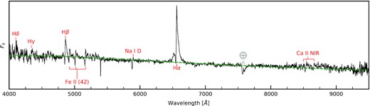
Classification spectrum of AT 2016jbu obtained with the Du Pont 2.5-m telescope and WFCCD (and reported in Bose et al. 2017) taken on 2016 December 31 (−31.4 d), corrected for reddening. This spectrum coincides with the approximate peak of Event A. The green dashed line is the blackbody fit with |$T_{BB}\, \sim$| 6750 K. H α and H β dominate the spectra and are both well fitted with a P Cygni profile with an additional emission component. We can also distinguish the Na i D lines superimposed on He i λ 5875 absorption. Fe ii λλ 4924,5018,5169 are present, all with a P Cygni profiles, giving a velocity at maximum absorption of ∼−700 km s−1. A noise spike at 5397 Å has been removed manually.
We present a single NIR spectrum taken in the low-dispersion and high-throughput prism mode with FIRE (Simcoe et al. 2013) mounted on one of the twin Magellan Telescopes (Fig. 16). The spectrum was obtained using the ABBA ‘nod-along-the-slit’ technique at the parallactic angle. Four sets of ABBA dithers totalling 16 individual frames and 2028.8 s of on-target integration time were obtained. Details of the reduction and telluric correction process are outlined by Hsiao et al. (2019).
In addition, we present two spectra taken with Gemini South + Flamingos2 (Eikenberry et al. 2006) in long-slit mode. An ABBA dither pattern was used for observations of both AT 2016jbu and a telluric standard. These data were reduced using the gemini.f2 package within iraf. A preliminary flux calibration was made using the telluric standard on each night (in both cases a Vega analogue was observed), and this was then adjusted slightly to match the J − H colour of AT 2016jbu from contemporaneous NIR imaging.
Swift + UVOT spectra were reduced using the uvotpy python package (Kuin 2014) and calibrations from Kuin et al. (2015).
3 PHOTOMETRIC EVOLUTION
3.1 Overall evolution
We present our complete light curve for AT 2016jbu in Fig. 2 and given in Table A1, spanning from ∼10 yr before maximum brightness (MJD: 57784.4) to ∼1.5 yr after maximum light. K18 mainly focus on the time around maximum light up until +118 d. on AT 2016jbu. Our photometric coverage is much higher cadence and covers a wider wavelength range.
For the purpose of discussion, we adopt the nomenclature for features seen in the light curve of SN 2009ip from Graham et al. (2014): rise, decline, knee, and ankle. We do not designate a ‘bump’ phase as while SN 2009ip shows a clear bump at ∼ 20 d, this is not seen in AT 2016jbu. The rise begins at ∼+ 22 d prior to V-band maximum. The decline phase begins at V-band maximum. The plateau begins at ∼+20 d, when the decline gradient flattens out initially. The knee stage is ∼+45 d past maximum when a sharp drop is seen in the light curve, and the ankle is the flattening of the light curve after ∼65 d before the seasonal gap.
AT 2016jbu shows a clear double-peaked light curve which has been previously missed in literature. The first fainter peak (at MJD 57751.2, mainly seen in rband) will be referred to as ‘Event A’, and the subsequent brighter peak is ‘Event B’. Event A is first detected around 3 months (phase: −91 d) before the Event B maximum in VLT + FORS2 imaging (Fraser et al. 2017). Phases presented in this paper for AT 2016jbu and other SN 2009ip-like transients will always be in reference to Event B maximum light (MJD 57784.4). The rise and decline of this first peak is clearly seen in r band (mainly detected from the Prompt telescope array) and sparsely sampled by Gaia in G band. Event A has a rise time to peak of ∼ 60 d, reaching an apparent magnitude r ∼ 18.12 mag (absolute magnitude −13.96 mag). We then see a short decline in r band for ∼ 2 weeks until AT 2016jbu exhibits a second sharp rise seen in all photometric bands, starting on MJD 57764.
We regard the start of this rise as the beginning of Event B. The second event has a faster rise time of ∼19 d, peaking at r ∼ 13.8 mag (absolute magnitude −18.26 mag). Our high-cadence data show after ∼20 d past the Event B maximum, a flattening is seen in Sloan-gri and Cousins BV that persists for ∼ 2 weeks, with a decline rate |$\sim 0.04\, {\rm mag\, d^{-1}}$|. At ∼50 d, a rapid drop is seen at optical wavelengths, with the drop being more pronounced in the redder bands and less in the bluer bands. After the drop there is a second flattening. After 2 months from the Event B peak, the optical bands flatten out with a decay of ∼0.015 mag d−1 and remain this way until the seasonal gap at ∼120 d.
Our data set includes late-time coverage of AT 2016jbu not previously covered in the literature. A rebrightening event is seen after ∼120 d and is seen clearly in BVGgr bands. We miss the initial rebrightening event in our ground-based data, so it is unclear if this is a plateau lasting across the seasonal gap or a rebrightening event. However, evidence for a rebrightening in the light curve is seen in Gaia-G (See Fig. 2). We can deduce that this event occurred between +160 and +195 d from our Gaia-G data, where we have G = 18.69 mag at +160 d, but an increase to 18.12 mag 1 month later. An additional bump is seen in Gaia-G at +345 d. We observe G = 18.95 mag at +316 d and G = 18.88 mag at + 342 d before AT 2016jbu fades to G = 19.72 mag a month later.
Late-time bumps and undulations in the light curves of SNe are commonly associated with late-time CSM interaction, when SN ejecta collide with dense stratified and/or clumpy CSM far away from the progenitor, providing a source of late-time energy (Fox et al. 2013; Martin et al. 2015; Arcavi et al. 2017; Nyholm et al. 2017; Andrews & Smith 2018; Moriya, Mazzali & Pian 2020).
3.2 Colour evolution
There exists a growing sample of SN 2009ip-like transients which evolve almost identically in terms of their photometry and spectroscopy, in the years prior to, and during their main luminous events.
The colour evolution of AT 2016jbu is discussed by K18. However, we include colour information prior to Event B maximum. Additionally, we show late-time colour evolution of K18.
In addition to AT 2016jbu, we focus on a small sample of objects that show common similarities to AT 2016jbu. For the purpose of a qualitative study, we will compare AT 2016jbu with SN 2009ip (Fraser et al. 2013; Graham et al. 2014), SN 2015bh (Elias-Rosa et al. 2016; Thöne et al. 2017), LSQ13zm (Tartaglia et al. 2016), SN 2013gc (Reguitti et al. 2019), and SN 2016bdu (Pastorello et al. 2018). We will refer to these transients (including AT 2016jbu) as SN 2009ip-like transients.
We also include SN 1996al (Benetti et al. 2016) in our SN 2009ip-like sample. Although no pre-explosion variability or an Event A/B light curve was detected, SN 1996al shows a similar bumpy decay from maximum and a similar spectral evolution as well as showing no sign of explosively nucleosynthesized material; e.g. |$[\mathrm{ O}\, \small{\rm I}]~\lambda \lambda ~6300,6364$| even after 15 yr. A modest ejecta mass and restrictive constraint on the ejected 56Ni mass are similar to what is found for AT 2016jbu and other SN 2009ip-like transients, see Paper II. Benetti et al. (2016) suggest that this is consistent with a fall-back SN in a highly structured environment, and we discuss this possibility for AT 2016jbu in Paper II.
We will also discuss SN 2018cnf (Pastorello et al. 2019); a previously classified Type IIn SN (Prentice et al. 2018). Although Pastorello et al. (2019) argue that SN 2018cnf displays many of the characteristics of SN 2009ip, it does not show the degree of asymmetry in H α when compared to AT 2016jbu but does show pre-explosion variability and general spectral evolution similar to SN 2009ip-like transients.
Fig. 4 shows that all these transients show a relatively slow colour evolution, typically seen in Type IIn SNe (Taddia et al. 2013; Nyholm et al. 2020). Where colour information is available, SN 2009ip-like transients initially appear red ∼1 month before maximum light, becoming bluer as they rise to maximum light. This is best seen in (B − V)0 for AT 2016jbu, SN 2015bh, and SN 2009ip. These three transients span colours from (B − V)0 ∼0.5 at ∼−20 d to ∼0.0 at ∼−10 d. In general, after the peak of Event B the transients begin to cool and again evolve towards the red.
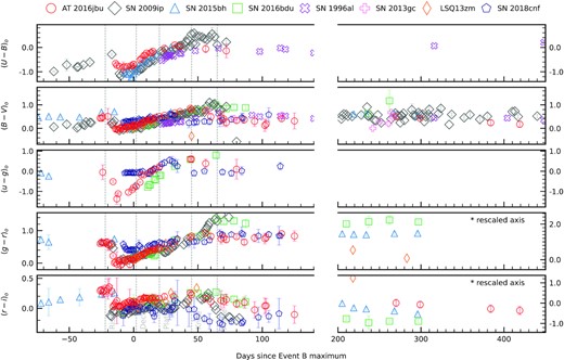
Intrinsic colour evolution of AT 2016jbu and SN 2009ip-like transients. All transients have been corrected for extinction using the values from Table A2. X-axis gives days from Event B maximum light. We include a broken X-axis to exclude the seasonal gap for AT 2016jbu. The data shown for AT 2016jbu have been regrouped into 1 d bins and weighted averaged. Error bars are shown for all objects, and we do not plot any point with an uncertainty greater than 0.5 mag. The different stages of evolution of AT 2016jbu are marked with grey dashed vertical bands.
For the first ∼20 d after Event B, AT 2016jbu follows the trend of other transients, which is seen clearly in (U − B)0, (B − V)0, (g − r)0, and (r − i)0. At ∼ 20 d AT 2016jbu flattens in (U − B)0 and (r − i)0, similar to SN 1996al and SN 2018cnf, whereas SN 2009ip flattens at ∼40 d in (U − B)0. This phase corresponds with the plateau stage in AT 2016jbu. This feature is also seen in (r − i)0 and (u − g)0, where AT 2016jbu plateaus at ∼20 d and then slowly evolves to the blue.
This behaviour is also seen in (B − V)0 and (g − r)0, where a colour change is observed at ∼50 d, followed by AT 2016jbu remaining at approximately constant colour until the seasonal gap at ∼120 d.
SN 2018cnf follows the trend of AT 2016jbu quite closely in (B − V)0 but this abrupt transition to the blue is seen at ∼30 d in SN 2018cnf, and ∼60 d in AT 2016jbu. AT 2016jbu and SN 2018cnf are distinct in their (g − r)0 evolution, as they match SN 2009ip and SN 2016bdu closely until ∼50 d, after which AT 2016jbu remains at an approximately constant colour, while SN 2009ip and SN 2016bdu make an abrupt shift to the red.
Filters that cover H α (viz. r,V) show an abrupt colour change at ∼60 d in AT 2016jbu (i.e. (B − V)0, (g − r)0, and (r − i)0), whereas those that do not cover H α show a similar feature at ∼30 d i.e. (U − B)0 and (u − g)0. As noted by K18, at this time we see an increase in the relative strength of the H α blue shoulder emission component (see Section 4.1). (B − V)0, (g − r)0, and (r − i)0 do not show this trend but rather a transition to the blue at ∼ 60 d. At late times, >120 d, AT 2016jbu remains relatively blue and follows the trends of other SN 2009ip-like transients, especially in (B − V)0.
3.3 Ground-based pre-explosion detections
A trait of SN 2009ip-like transients is erratic photometric variability12 in the period leading up to Event A and Event B.
The lower panel of Fig. 2 shows all pre-Event A/B observations for AT 2016jbu from ground-based instruments. The majority of these observations are from the PROMPT telescope array, and have been host subtracted using late time r-band templates from EFOSC2. Unfortunately, these images are relatively shallow. In addition, we recovered several images from the LCO network which were obtained for the follow-up campaign of SN 2015F (Cartier et al. 2017). These images have been host subtracted using templates from LCO taken in 2019. We also present several images taken from VLT + OMEGAcam, which are deeper than our templates and are hence not host subtracted. For completeness, we also plot detections of the progenitor of AT 2016jbu from HST in Fig. 2, which we discuss in Paper II.
If AT 2016jbu underwent a similar series of outbursts prior to Event A/B as seen in other SN 2009ip-like transients, then we would expect to only detect the brightest of these. SN 2009ip experiences variability at least 3 yr prior to its main events.
For AT 2016jbu, several significant detections are found with r∼ 20 mag in the years prior to Event A/B. For our adopted distance modulus and extinction parameters, these detections correspond to an absolute magnitude of Mr ∼ −11.8 mag. Similar magnitudes were seen in SN 2009ip and SN 2015bh, see Fig. 17. SN 2009ip was observed with eruptions exceeding R ∼ −11.8 mag, with even brighter detections for SN 2015bh.
Both SN 2009ip and SN 2015bh show a large increase in luminosity ∼450 d prior to their Event A/B. The AT 2016jbu progenitor is seen in HST images around −400 d showing clear variations. A single DECam image in r band gives a detection at r ∼ 22.28 ± 0.26 mag at −352 d, which roughly agrees with our F350LP light curve at this time (if we presume H α is the dominant contributor to the flux). We present and further discuss HST detections inPaper II.
We note that we detect a point source at the site of AT 2016jbu in several PROMPT images but not in any of the LCO, WFI, NTT+EFOSC2/SOFI, OmegaCAM, or VISTA+VIRCAM pre-explosion images. However, a clear detection is made with CTIO + DECAM that is compatible with our HST observations (see Paper II for more discussion of this).
In Fig. 5, we show a selection of cut-outs from our host-subtracted PROMPT images, showing the region around AT 2016jbu. While some of the detections that AutoPhOT recovers are marginal, others are quite clearly detected, and so we are confident that the pre-discovery variability is real. If these are indeed genuine detections, then AT 2016jbu is possibly undergoing rapid variability similar to SN 2009ip and SN 2015bh in the years leading up to their Event A. The high cadence of our PROMPT imaging and the inclusion of H α in the Lum filter plausibly explain why we have not detected the progenitor in outburst in data from any other instrument.
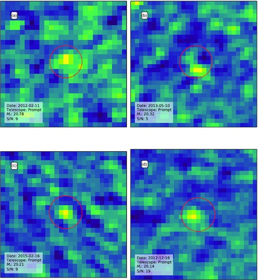
Sample of pre-explosion detections from PROMPT at the progenitor location. Centre of cut-out corresponds to AT 2016jbu progenitor location. The red circle signifies aperture with radius 1.3 × FWHM placed in the centre of the cut-out. As mentioned in Section 2.1, these unfiltered images have been host subtracted using r-band templates. Template subtractions performed using AutoPhOT and hotpants (Becker 2015), see Section 2.6.
AT 2016jbu could be undergoing a slow rise up until the beginning of Event A similar to UGC 2773-OT (Smith et al. 2016) (Intriguingly this is also seen in Luminous Red Novae, Pastorello et al. 2021; Williams et al. 2015 – we return to this in Paper II). Fitting a linear rise to the PROMPT pre-explosion detections (i.e. excluding the HST and DECam detections) gives a slope of −5.4 ± 1 × 10⁻⁴ mag d−1 and intercept of 19.07 ± 0.19 mag. If we extrapolate this line fit to −60 d (roughly the beginning of r-band coverage for Event A) we find a value of rextrapolate ∼ 19.11 mag which is very similar to the detected magnitude at −59 d of r ∼ 19.09 mag. However, this is speculative, and accounting for the sporadic detections in the preceding years, and the non-detections in deeper images e.g. from LCO see lower panel of Fig. 2, it is more likely that AT 2016jbu is undergoing rapid variability (similar to SN 2009ip) which is serendipitously detected in our PROMPT images due to their high cadence.
3.4 UV observations
Fig. 6 shows Swift + UVOT observations around maximum light. All bands show a sharp increase at ∼−18 d, consistent with our optical light curve. The Swift + UVOT can constrain the initial Event B rise to some time between ∼−18.6 and ∼−16.2 d.
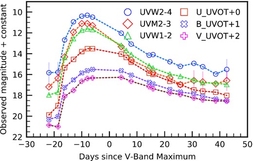
Swift + UVOT light curve for AT 2016jbu. All photometry is host subtracted. Offsets are given in the legend and uncertainties are included for all points.
The decline of the UV light curve is smooth and does not show any obvious features up to +45 d. UVW2 shows a possible bump beginning at ∼24 d that spans a few days. This bump is also evident in UVM2 at the same time. This bump is consistent with the emergence of a blue shoulder emission in H α (See Section 4.1) and it is possible that we are seeing an interaction site between ejecta and CSM at this time.
3.5 X-ray observations
No clear X-ray source was found consistent with the location of AT 2016jbu in the XMM data taken at −5 d. Using the sosta tool on the data from the PN camera we obtain a 3σ upper limit of <3.2 × 10⁻³ counts s−1 for AT 2016jbu, while the summed MOS1 + MOS2 data give a limit of <2.1 × 10⁻³ counts s−1. Assuming a photon index of 2, the upper limit to the observed flux in the 0.2–10 keV energy range is 1.2 × 10⁻¹⁴ erg cm−2 s−1.
For comparison, SN 2009ip was detected in X-rays in the 0.3–10 keV energy band with a flux of (1.9 ± 0.2) × 10−14 erg cm−2 s−1, as well as having an upper limit on its hard X-ray flux around optical maximum (Margutti et al. 2014).
X-ray observations can tell us about the ejecta–CSM interaction as well as the medium into which they are expanding into (Dwarkadas & Gruszko 2012). The non-detection for AT 2016jbu provides little information on the nature of Event A/B. Making a qualitative comparison to SN 2009ip we note that AT 2016jbu is not as X-ray bright, and this may reflect different explosion energies, CSM environments or line-of-sight effects.
3.6 MIR evolution
We measure fluxes for AT 2016jbu in Spitzer IRAC Ch1 = 0.123 ± 0.003 mJy and Ch2 = 0.136 ± 0.003 mJy, which are roughly consistent with those found by K18. This corresponding to magnitudes of 16.00 and 15.25 for Ch1 and Ch2, respectively. Neither this work nor K18 find evidence for emission from cool dust in Ch3 and Ch4 at the progenitor site of AT 2016jbu.
We further discuss the evidence for a dust-enshrouded progenitor in Paper II but here we briefly report the findings from K18. Coupled with pre-explosion HST observations, K18 find that the progenitor of AT 2016jbu is consistent with the progenitor system having a significant IR excess from a relatively compact, dusty shell. The dust mass in the immediate environment of the progenitor system is small (a few × 10−6 M⊙). However, the different epochs of the HST (taken in 2016) and Spitzer (taken in 2003) data suggest they may be at different phases of evolution. Fig. 2 shows that the site of AT 2016jbu underwent multiple outbursts between 2006 and 2013, and, as mentioned by K18, fitting a single SED to the HST and Spitzer data sets may be somewhat misleading.
4 SPECTROSCOPY
We present our high-cadence spectral coverage of AT 2016jbu in Fig. 7. Our spectra begin at −31 d and show an initial appearance similar to a Type IIn SN, i.e. narrow emission features seen in H and a blue continuum. Our first spectra coincide with the approximate peak of Event A. After around a week, additional absorption and emission features emerge in the Balmer series, which we illustrate in Fig. 8 and plot the evolution of in Fig. 9. The spectrum does not vary significantly over the first month of evolution aside from the continuum becoming progressively bluer with time. H α shows a P Cygni profile with an emission component with FWHM ∼ 1000 km s−1and a blue shifted absorption component with a minimum at ∼−600 km s−1. The narrow emission lines likely arise from an unshocked CSM environment around the progenitor. Over time AT 2016jbu develops a multicomponent emission profile seen clearly in H α that persists until late times. We do not find any clear signs of explosively nucleosynthesized material at late times, and indeed the spectral evolution appears to be dominated by CSM interaction at all times. We discuss the evolution of the Balmer series in Section 4.1. In Section 4.2, we discuss the evolution of |$\mathrm{ Ca}\, \small {\rm II}$| features and model late-time emission profiles. Section 4.3 discusses the evolution of several isolated, strong iron lines. Section 4.4 discusses the evolution of |$\mathrm{ He}\, \small{\rm I}$| emission and makes qualitative comparisons between |$\mathrm{ He}\, \small{\rm I}$| features and the optical light curve. We present UV and NIR spectra in Section 4.6 and Section 4.7, respectively.
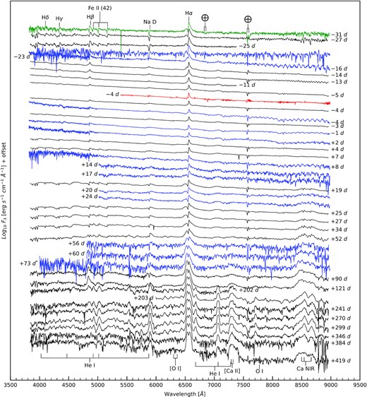
Spectral evolution of AT 2016jbu. Wavelength given in rest frame. Flux given in log scale. Prominent spectral lines and strong absorption bands are labelled. Colours instruments used (see Table 1); black: NTT+EFOSC2, blue: FTS + FLOYDS, red: WiFeS, green: DuPont. Spectra marked with an asterisk have been smoothed using a Gaussian filter of FWHM 1 Å.
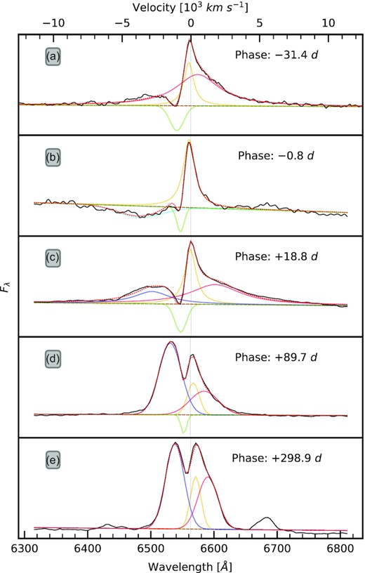
Multicomponent evolution of H α over a period of ∼1 yr. We use Lorentzian emission and Gaussian absorption profiles at early times (phase <+ 120 d), and Gaussian emission and absorption thereafter. Epochs are given in each panel, lines are coloured such that yellow = core emission, red = redshifted emission, green = P-Cygni absorption, cyan = high-velocity absorption, and blue is blueshifted emission. In panel A, an additional emission component could be included to account for the blue excess shown, although this can simply be extended electron scattering wings.
4.1 Balmer line evolution
The most prominent spectral features are the Balmer lines, which show dramatic evolution over time. In particular the H α profile, which shows a complex, multicomponent evolution, provides insight to the CSM environment, mass-loss history, and explosion sequence. Although SN 2009ip never displayed obvious multicomponent emission features, a red-shoulder emission is seen at late times (Fraser et al. 2013). We present the evolution of H α for AT 2016jbu at several epochs showing the major changes in Fig. 8.
K18 discuss the evolution of the H α in detail out to +118 d. With our high-cadence spectral evolution we preform a similar multicomponent analysis while focusing on individual feature evolution.
Similar to K18, we conducted spectral decomposition to understand line shape and the ejecta–CSM interaction. We used a Markov Chain Monte Carlo approach for fitting a multicomponent spectral profile (Newville et al. 2014) using a custom python3 script. When fitting, absorption components are constrained to be blueward of the rest wavelength of each line to reflect a P Cygni absorption. All lines are fitted over a small wavelength window and we include a pseudo-continuum during our fitting, which is allowed to vary. Fitting the H α evolution is performed on each spectrum consecutively, using the fitted parameters from the previous model as the starting guess for the next. This is reset after the observing gap at +202 d. Fig. 8 presents fitted models to the H α profile at epochs where significant change are seen. The FWHM and peak wavelength for H α are illustrated in Fig. 9.

Evolution of fitted parameters for H α. The upper panel shows the absolute velocity evolution of each feature. We fit a power decay law with index 0.4 dex to the blue emission from when it first appears (∼+18d) until the seasonal gap (∼+ 125 d) indicated by the blue dashed line. The is also fitted for the red shoulder emission (with a different normalization constant) as the red dashed line. We include a purple dotted line at 1200 km s−1that matches the late-time red and blue emission components. The lower panel shows the FWHM evolution of each of the components. We do not plot the redshifted broad emission fitted during the first three epochs in either panel.
Days −31 to −25: Similar to K18, our first spectrum coincides with the approximate peak of Event A (Fig. 2). H α can be modelled by a P Cygni profile with an absorption minimum at ∼−700 km s−1 superimposed on a broad component at ∼+700 km s−1with an FWHM of ∼2600 km s−1. This can be interpreted as a narrow P Cygni with extended, electron-scattering wings, as often seen in Type IIn SN spectra (see review by Filippenko 1997).
Days −14 to +4: We see a gradual decay in amplitude of the core broad emission until we find a best fit by a single intermediate-width Lorentzian profile (FWHM ∼ 1000 km s−1) and P Cygni absorption. Our Lorentzian profile has broad wings, possibly due to electron scattering along the line of sight (Chugai 2001). For further discussion, see K18.
At −14 d, a blue broad absorption component clearly emerges at ∼−5000 km s−1with an initial FWHM of ∼3800 km s−1, with the fastest material is moving at ∼10 000 km s−1. This feature was not seen in K18 due to a lack of observations at this phase. The trough of this absorption features slows to ∼−3200 km s−1 at +3 d. Panel B in Fig. 8 shows H α at −1 d with a strong Lorentzian emission with the now obvious blue absorption. This feature indicates that there is fast-moving material that was not seen in the initial spectra. Assuming free expansion, we set an upper limit on the distance travelled by this material to |$\sim 2.5\times 10^{15}\, {\rm cm}$|.
A similar feature was also seen in SN 2009ip (e.g. fig. 2 of Fraser et al. 2013) around the Event B maximum. A persistent second absorption feature was also seen in SN 2015bh (Elias-Rosa et al. 2016), which remained in absorption until several weeks after the Event B maximum, when it was replaced by an emission feature at approximately the same velocity.
Days +7 to +34: A persistent P Cygni profile is still seen but a dramatic change is seen in the overall H α profile, now being dominated by a red-shifted broad Gaussian feature centred at ∼+2200 km s−1 and FWHM ∼4000 km s−1. The blue absorption component has now vanished and been replaced with an emission profile with a slightly lower velocity, −2400 km s−1 at + 18 d, seen in panel C of Fig. 8. Over the following month, this line moves towards slower velocities with a decreasing FWHM. The blue shoulder emission is clearly seen at ∼+18 d and remains roughly constant in amplitude (with respect to the core component) until ∼+34 d. At +34 d this line now has an FWHM ∼ 2700 km s−1. By +52 d this blue emission line has grown considerably in amplitude with respect to the core component. During this period the relative strength of the red and blue component begins to change, indicating on-going interaction and/or changing opacities. We note that prior to +52 d, this H α profile may be fitted with a single, broad emission component with a P Cygni profile. However, during our fitting a significant blue excess was always present during +7 to +34 d. Allowing for both a blue and red emission component during these times allows each consistent component to evolve smoothly into later spectra, as is seen in Figs 8 and 9.
Days +52 to +120: As mentioned in by K18, H α shows an almost symmetric double-peaked emission profile. The earliest profile of H α at −31 d is reminiscent of some stages during an eruptive outburst from a massive star (for example Var C; Humphreys et al. 2014). We plot the profile of the +90 d profile in Fig. 10 with a blue-shifted Lorentzian profile removed. The profiles are very similar in overall shape with a slightly broader red-core component in the +90 d spectrum. A possible interpretation is the P Cygni-like profile seen in our −31 d spectra is associated with the events during/causing Event A (for example a stellar merger or eruptive outburst) and the blue side emission is associated with events during/causing Event B (for example a core-collapse or CSM interaction).
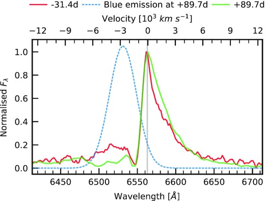
H α profile at −31 d (red) and +90 d (green) for AT 2016jbu. The +90 d profile has had a strong blue emission profile (given by dotted blue line) subtracted and we plot the residual in green. Each spectra is normalized at 6563 Å. The profile at +90 d has been blue-shifted by 4Å (∼−180 km s−1) to match the peak at the H α rest wavelength (6563 Å) of the profile at −31 d.
Days +203 to +420: We present late-time spectra of AT 2016jbu not previously covered in the literature. The red and blue components of the H α profile now have similar FWHM of ∼2100 and ∼1600 km s−1, respectively. The overall H α profile has retained its symmetric appearance (panel D of Fig. 8). After this time we no longer fit a P Cygni absorption profile, and our spectra can be fitted well using three emission components. We justify this as any opaque material may have become optically thin after ∼7 months and the photospheric phase has ended.
Little evolution in H α is seen for the remainder of our observations. The three emission profiles remain at their respective wavelengths and the approximate same width. The overall evolution of H α suggests that AT 2016jbu underwent a large mass-loss event (whether that be an SN or extreme mass-loss episode) in a highly aspherical environment. Interaction with dense CSM forming a multicomponent H α profile as well as a bumpy light curve.
4.2 Calcium evolution
Section 4.1 indicates that AT 2016jbu has a highly non-spherical environment. We investigate similar trends in other emission profiles. K18 suggest that the [Ca ii] and Ca ii NIR triplet may be coming from separated regions. Motivated by this, we explore the Ca ii NIR triplet λλλ 8498, 8542, 8662 using the same method in Section 4.1. The Ca ii NIR triplet appears in emission at approximately the same time as blue-shifted emission in H α (∼+18 d) and at early times shows P Cygni absorption minima at velocities similar to H α. For profile fitting, the wavelength separation between the three components of the NIR triplet was held fixed, while the three components were also constrained to have the same FHWM. Amplitude ratios between the three lines were constrained to physically plausible values between the optically thin and optically thick regimes (Herbig & Soderblom 1980).
The early evolution of the Ca ii NIR triplet is detailed in K18. We explore two scenarios for the Ca ii NIR triplet evolution after +200 d. In the first, we assume that the Ca ii emission comes from the same regions as H α (as suggested in Section 4.1) i.e. two spatially separated emitting regions. We allow the first region to be fitted with the above restrictions (fixed line separation, single common FWHM), we refer to this as Region A. A second, kinematically distinct, multiplet is added (we refer to this as Region B) and simultaneously fitted with additional constraints; the lines have the same FWHM as the region A and the amplitude ratio of the Ca ii NIR triplet being emitted from region B is some multiple of the region A. Region B represents this blue-shifted material seen in H α. The second scenario has an additional Gaussian representing |$\mathrm{ O}\, \small{\rm I}~\lambda 8446$| fitted independently to a single Ca ii emitting region.
As shown in Fig. 11, both scenarios give an acceptable fit to spectrum at +345 d. Fitting a single Gaussian emission line representing |$\mathrm{ O}\, \small{\rm I}~\lambda 8446$| gives a reasonable fit with FWHM ∼ 4000 km s−1redshifted by ∼800 km s−1. Alternatively, adding an additional Ca ii emission profile we find a good fit at FWHM ∼ 2000 km s−1and blue-shifted by ∼−2800 km s−1. Although the scenarios are inconclusive, this does not exclude a complex asymmetrical CSM structure producing these multiple emitting regions along the line of sight.
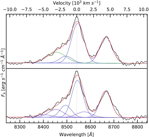
Calcium NIR triplet fit for +345 d. The individual components of the primary Ca ii NIR triplet is given by the blue dashed lines in both plots. The upper panel shows the emission profile with the inclusion of |$\mathrm{ O}\, \small{\rm I}~\lambda 8466$| (in green). The lower panel shows the model fit in blue (Region A) with the second region of Ca ii NIR triplet emission shown in purple (Region B). Both |$\mathrm{ O}\, \small{\rm I}~\lambda 8466$| and a second region of Ca emission give a similarly acceptable fit to the data.
Although both scenarios give reasonable fits, the FWHM and velocities deduced for both scenarios are not seen elsewhere in the spectrum at +345 d. It is possible that the region(s) producing the Ca ii NIR triplet is separated from H-emitting areas although detailed modelling is needed to confirm. We note however one should expect a similar flux from |$\mathrm{ O}\, \small{\rm I}~\lambda 7774$| when assuming the presence of |$\mathrm{ O}\, \small{\rm I}~\lambda 8446$|, which is not the case here. If both lines are produced by recombination, we expect similar relative intensities (Kramida et al. 2020). Interestingly, this is also trend is also seen in SN 2009ip (Graham et al. 2014).
Our final spectra on +385 d and +420 d show the Ca ii NIR triplet and [Ca ii] having a broadened appearance compared to earlier spectra. This may indicate an increase in the velocity of the region where these lines form, similar to what is seen in H α in Section 4.1.
4.3 Iron lines
As temperatures and opacities drop the spectra of many CCSNe become dominated by iron lines, as well as Na i and Ca ii. We notice persistent permitted Fe group transitions throughout the evolution of AT 2016jbu, which is likely pre-existing iron in the progenitor envelope. Our initial spectra display the |$\mathrm{ Fe}\, \small {\rm II} ~\lambda \lambda \lambda ~4924,5018,5169$| (multiplet 42) as P Cygni profiles, see Fig. 3. At −31 d we measure the absorption minimum of Fe ii multiplet 42 at −750 km s−1. This is the same velocity as the fitted absorption profile from H α/H β see Fig. 8 A. We can assume that this lines originate in similar regions.
The Fe ii multiplet 42 appears in our late-time spectra, see Fig. 12. Fe ii lines in general appear with P Cygni profiles at late times. It is difficult to measure the absorption minimum of the Fe ii profile due to severe blending. However, using several relatively isolated Fe ii lines at +345 d we measure an absorption minimum of ∼−1300 km s−1. The values is similar to the velocity offset for the red and blue emission components seen in H α. This suggest that these lines are originating in the same region.
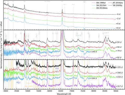
Spectral comparison of SN 2009ip-like transients around Event B peak (top), 3 months after Event B (middle), and late-time spectra around 1 yr later (bottom). We include several strong Fe ii emission lines in the bottom panel as orange vertical lines. We note the remarkable similarities between AT 2016jbu and other SN 2009ip-like transients at late times.
4.4 Helium evolution
None of the He i lines display the degree of asymmetry seen in hydrogen. Transients exist displaying double-peaked helium lines, such as the Type Ibn SN 2006jc; (Foley et al. 2007; Pastorello et al. 2008), as well as some displaying asymmetric He i and symmetric H emission e.g. the Type Ibn/IIb SN 2018gjx (Prentice et al. 2020).
We show the evolution of |$\mathrm{ He}\, \small{\rm I} ~\lambda 5876$| (black line) and |$\mathrm{ He}\, \small{\rm I} ~\lambda 7065$| (green line) in Fig. 13. |$\mathrm{ He}\, \small{\rm I} ~\lambda 7065$| first appears in emission on −14 d with a boxy profile that is poorly fit with a single Lorentzian emission line. |$\mathrm{ He}\, \small{\rm I} ~\lambda 7065$| then becomes more symmetric by +18 d. Note the blue absorption feature in H α is also first seen at this time. The line begins to broaden over the next month, peaking at FWHM ∼ 3400 km s−1 at ∼+28 d. After +51 d, |$\mathrm{ He}\, \small{\rm I} ~\lambda 7065$| is no longer detected with any reasonable S/N.
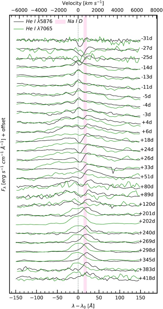
Evolution of |$\mathrm{ He}\, \small{\rm I}~\lambda 5876$| (black) and |$\mathrm{ He}\, \small{\rm I}~\lambda 7065$| (green) from NTT + EFOSC2 and DuPont spectra. The rest wavelength of the |$\mathrm{ He}\, \small{\rm I}$| lines (5876 and 7065 Å) are marked with a vertical line, while Na i D λλ 5890, 5895 is shown by the red vertical band. A velocity scale for the |$\mathrm{ He}\, \small{\rm I}$| lines is given in the upper axis. Each spectrum has been normalized to a peak value of unity.
Interestingly, |$\mathrm{ He}\, \small{\rm I} ~\lambda 7065$| then re-emerges at +200 d, the emission feature has FWHM ∼ 1100 km s−1 centred at rest wavelength. We see this same FWHM in the red and blue shoulders in H α (Section 4.1). We find that a single emission profile matches the |$\mathrm{ He}\, \small{\rm I} ~\lambda 7065$| line well after +200 d. However, motivated by the multicomponent profile of H α we also find that |$\mathrm{ He}\, \small{\rm I}~\lambda 7065$| after +200 d can be fitted equally well with two emission components. In this case, both components are offset by ∼±400 km s−1from their rest wavelength, and each has an FWHM of ∼1000 km s−1. Unlike H α, no third core emission component is needed.
For |$\mathrm{ He}\, \small{\rm I} ~\lambda 5876$|, in our −31 d spectrum there is a clear P Cygni profile centred at 5898 Å. The emission is likely caused by Na i D with the possibility of some absorption contamination from |$\mathrm{ He}\, \small{\rm I} ~\lambda 5876$|. We measure a velocity offset of ∼−450 km s−1with respect to 5890 Å. At −13 d, |$\mathrm{ He}\, \small{\rm I} ~\lambda 5876$| emerges and has a complicated, multicomponent profile with contamination from Na i D. Emission centred on 5876 Å persists until +20 d, after which the emission returns to being dominated by Na i D.
Low-resolution spectra preclude further investigation, but if |$\mathrm{ He}\, \small{\rm I}~\lambda 7065$| is composed of two emission profiles, these two emission regions are at significantly lower velocity when compared to the similar components in H α. An increase in the strength of He i was also seen in the Type IIn SN 1996al and was interpreted as a signature of strengthening CSM interaction (Benetti et al. 2016).
|$\mathrm{ He}\, \small{\rm I} ~\lambda 6678$| evolves in a similar manner to |$\mathrm{ He}\, \small{\rm I} ~\lambda 7065$|, but shows a clear P Cygni profile as early as −14 d with an absorption trough at ∼−500 km s−1, similar to H α. After the seasonal gap |$\mathrm{ He}\, \small{\rm I}~\lambda 5876$| is not clearly seen. At +345 d we measure a Gaussian emission profile centred at 5897 Å with an FWHM ∼ 1800 km s−1. This is likely dominated by Na i D with minor contamination from |$\mathrm{ He}\, \small{\rm I}~\lambda 5876$|. The FWHM value for this line suggests that it is coming from the site of AT 2016jbu and not due to host contamination.
We plot the evolution of the pseudo-Equivalent Width (pEW) (a pseudo-continuum is fitted over a small wavelength window) of the two seemingly isolated |$\mathrm{ He}\, \small{\rm I}~\lambda \lambda ~6678,7065$| emission lines in Fig. 14. We note that there is little change in pEW for the first ∼120 d. After the seasonal gap, both emission lines increase dramatically in pEW, until ∼+ 300 d after which the pEW declines. A similar jump in He i was seen in SN 1996al (Benetti et al. 2016). This decline coincides with the narrowing and increase in amplitude of the blue, red, and core emission components of H α.
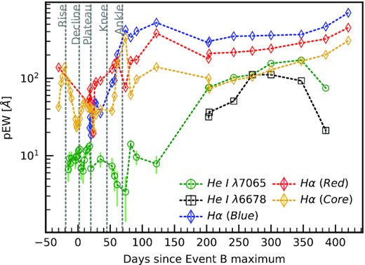
Evolution of pEW for |$\mathrm{ He}\, \small{\rm I}~\lambda ~6678, \lambda ~7065$| and H α components. The He i emission appears to be roughly constant until the knee/ankle stage when it increases rapidly. After ∼+ 300 d the pEW of He i again begins to decrease. The measurement of pEW is based on a single emission component fit which provides a reasonable fit at late times. |$\mathrm{ He}\, \small{\rm I}~\lambda ~6678$| is not plotted for t < 220 d due to its low pEW and contamination from H α.
He i emission is expected to be formed in the de-excitation/recombination region of the shock wave (Chevalier & Kirshner 1978; Gillet & Fokin 2014). As mentioned in Section 4.1, after ∼ 2 months, the blue shifted emission in H α grows in amplitude and narrows considerably, likely due to changing opacities. This jump in pEW may represent a time when shocked material is no longer obscured and photons can escape freely from the interaction sites. We reach a similar conclusion for He i. If the trend in both He i lines is linked to the H α emitting regions, then it is likely that the late time He i might also be double-peaked.
Fig. 2 shows a rebrightening/flattening after the seasonal gap. This is seen best in Gaia-G. The trend seen in He i λ 6678 and λ 7065 pEW may follow the interaction of the shock front with some clumpy dense material far away from the progenitor site. This would reflect a stratified CSM profile possibly produced by the historic eruptions, or possibly a variable wind, in AT 2016jbu.
4.5 Forbidden emission lines
A clear sign of a terminal explosion is forbidden emission lines from material formed during explosive nucleosynthesis/late-time stellar evolution. All CCSNe will eventually cool down sufficiently for the photosphere to recede to the innermost layers of the explosion. We expect to see the signatures of material synthesized in the explosion as well as material produced in the late-stages of stellar evolution such as |$[\mathrm{ O}\, \small{\rm I}]~\lambda \lambda ~6300, 6364$| or |$\mathrm{ Mg}\, \small{\rm I}]~\lambda ~4571$| (Jerkstrand 2017).
Fig. 12 shows the late-time spectra of AT 2016jbu highlighting prominent emission lines. Tenuous detections are made of [O i] and Mg i], although these lines are much weaker than are typically seen during the nebular phase of CCSNe. Late-time spectra show that there is on-going CSM interaction for AT 2016jbu, as is clear for the double-peaked H α emission. The spectra are still relatively blue (i.e. Fig. 12, λ ≲5600 Å) even after 1 yr, again indicating interaction in the CS environment.
It is a common conclusion for SN 2009ip-like transients that there are only tenuous signs of core-collapse (Fraser et al. 2013; Benetti et al. 2016). Fraser et al. (2013) find no clear signs of any such material during the late-time nebular phase of SN 2009ip. SN 2009ip showed little indication of a nebular phase and in 2012 showed spectral features similar to its 2009 appearance. Benetti et al. (2016) find no evidence of nebular emission features in SN 1996al even after 15 yr of observations. For AT 2016jbu one may posit that if the transient is indeed a CCSNe, on-going interaction has led to densities too high for forbidden lines to form. Alternatively, fallback on to a compact remnant could result in an apparently small mass of synthesized heavy elements, and hence an absence of nebular CCSN features. We will expand further on the nature of AT 2016jbu and SN 2009ip-like transients, their powering mechanism, and the possibility that the progenitor survived, in Paper II.
4.6 UV spectrum
We present a single UV spectrum in Fig. 15 taken with Swift + UVOT on 2017 January 22. The spectrum has quite low S/N towards the red with a very tenuous detection of the Balmer series. It is likely that λ > 4000 Å is affected by second order contamination. The continuum of AT 2016jbu deviates significantly from a blackbody at short wavelengths (λ < 2400 Å) mainly due to blends of lines of singly ionized iron-peak elements.
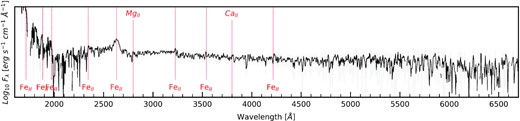
Swift + UVOT spectrum for AT 2016jbu taken on 2017 January 22 (MJD: 57775, Phase: −18 d). Wavelength in given in rest frame and the spectrum is corrected for Galactic extinction (AV = 0.556 mag). The spectrum is given in black with the grey shaded region showing the uncertainty. The trough around 2000 Å is likely noise which is likely exacerbated by our extinction correction.
A broad (FWHM ∼ 5000 km s−1) emission line is the strongest feature seen. It is centred at ∼2630 Å and is well fitted with a single Gaussian. We are unsure of the identification of this emission line, however there is a strong |$\mathrm{ Fe}\, \small {\rm II}$| line at ∼ 2631 Å (Nave et al. 1994; Kramida et al. 2020).
It is curious that there is a strong |$\mathrm{ Fe}\, \small{\rm II}$| line here and no other emission features at comparable strength. Swift observations of SN 2009ipdo show this emission line but it is much weaker than that seen in AT 2016jbu (Margutti et al. 2014). This particular emission line has been seen in several Type IIP SNe with UV coverage such as SN 1999em and SN 2005cs (see Gal-Yam et al. 2008, and references therein). However, the Type IIP SNe discussed by Gal-Yam et al. (2008) also show strong emission from |$\mathrm{ Mg}\, \small {\rm II}~\lambda ~2800$|. AT 2016jbu shows a weaker P Cygni feature centred at 2800 Å with an absorption at ∼−1200 km s−1, which is likely due to |$\mathrm{ Mg}\, \small {\rm II}~\lambda ~2800$|. Detailed spectral modelling is needed to secure this line identification.
4.7 NIR spectra
We present our NIR spectra in Fig. 16 covering the peak of Event A as well as the rise and peak of Event B. Paβ λ 12822 follows the same evolution as H α, with a strong blue absorption profile that is not present in the −31 d FIRE spectrum but which appears in the FLAMINGOS-2 − 12 d spectra. At this phase the blue absorption is already seen in H α and H β. Pa β is also broader at −31 d and narrows at −12 d, similar to the H α evolution shown in Fig. 8 at −31 d and +1 d.
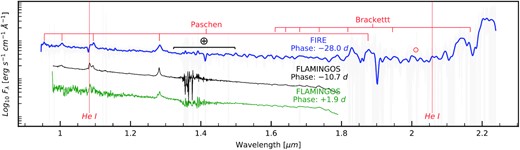
NIR spectra of AT 2016jbu, covering the peak of Event A as well as the rise and peak of Event B. H and He i are clearly seen in all spectra. The FIRE spectrum (blue) has been smoothed for presentation and shows what appears to be an excess redwards of 2.05 |$\mu$|m. This excess is likely due to spectra being saturated by the bright K-band sky.
There is a strong He i λ10830 line blended with Paγ. At −31 d this line appears in absorption at rest wavelength, while by −12 d the line is in emission. This helium feature may be thermally excited and this is supported by the blackbody temperature seen peaking at this time (see Paper II). We see an absorption trough bluewards of λ10830 which may be associated with Paγ λ 10941 (as a similar absorption is seen in Paβ). There appears to be a flux excess beyond 2.1 |$\mu$|m in the FIRE spectrum at −31 d. This may represent emission from a CO bandhead, possibly signifying some pre-existing dust during Event A. However, the S/N is extremely low in this region of the spectrum (see the grey shaded region in Fig. 16), and it is likely that the apparent ‘excess’ is due to bright K-band sky contamination rather than CO emission.
5 DISCUSSION
We will discuss AT 2016jbu and their relation to SN 2009ip-like objects, mainly their photometric similarities in Section 5.1.1 and their spectroscopic appearance in Section 5.1.2, in particular the appearance of their H α emission profiles is varies times during their evolution (Section 5.1.3).
5.1 AT 2016jbu and other SN 2009ip-like transients
For this paper, we focus the discussion on the photometric and spectral comparison between AT 2016jbu and similar transients. In Paper II, we discuss topics including the progenitor of AT 2016jbu using pre-explosion images, the environment around the progenitor, and a non-terminal explosion scenario.
5.1.1 Photometric comparison
We compare the R/r-band light curves of a sample of SN 2009ip-like transients events in Fig. 17. In cases where r-band photometry was not available, Johnson-Cousin R-band is shown. The adopted extinction and distance moduli are given in Table A2. The photometric evolution for SN 2009ip-like transients is undoubtedly similar. Our sample of transients all show a series of outbursts in the years prior to Event A, as seen in Fig. 17. This has been described as historic ‘flickering’ by K18. AT 2016jbu shows several clear detections within ∼10 yr before the peak of Event B. Similar outbursts are seen in other SN 2009ip-like transients (see Fig. 17).
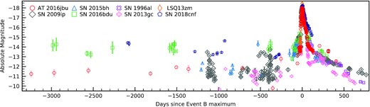
Pre-explosion outbursts and the main luminous event for the sample of SN 2009ip-like transients. SN 2009ip (Sloan r) is taken from Fraser et al. (2013), Graham et al. (2014), SN 2015bh(R) from Thöne et al. (2017), SN 2016bdu(r) from Pastorello et al. (2018), SN 2013gc(R) from Reguitti et al. (2019), SN 1996al(R) from Benetti et al. (2016), SN 2018cnf(r) from Pastorello et al. (2019), and LSQ13zm(R) is taken from Tartaglia et al. (2016). All data are given in Vega magnitudes (Blanton & Roweis 2007). We do not show limiting magnitudes in this figure for clarity. All events show an initial rise to a magnitude of ∼−14 (if coverage available) followed by a second rise to ∼−18 roughly 30 d later. Our sample of SN 2009ip-like transients all show outbursts in the months/years prior to their luminous events.
The duration of Event A varies between each transient. For SN 2009ip, Event A lasts for ∼1.5 months (Fraser et al. 2013) and rises to ∼−15 mag. LSQ13zm shows a rise to ∼−14.8 mag and has a time frame of a few weeks (Tartaglia et al. 2016). All transients show a fast rise of ∼ 17 d to maximum in Event B to ∼−18 ± 0.5 mag followed by a rapid/bumpy decay. Kiewe et al. (2012) found that a magnitude of −18.4 is typical for Type IIn SNe. Using a larger sample size, Nyholm et al. (2020) find a larger value for the mean value although Event B peak is still within a standard deviation of this.
Curiously, several of the transients in our sample show their first initial bump around the same time, approximately 20 d post maximum; see Fig. 18. AT 2016jbu shows no major bumps in its light curve, but instead flattens slightly, whereas SN 2009ip and SN 2018cnf show a clear and prominent bump at ∼20 d.
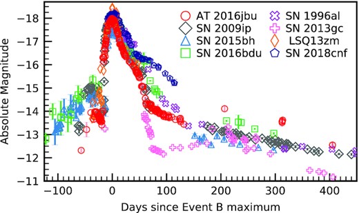
Same as Fig. 17, but focusing Event A/B. All SN 2009ip-like transients show a similar Event B (light curve), although Event A tends to be more diverse (if observations are available). AT 2016jbu shows a major rebrightening after ∼200 d not seen in other SN 2009ip-like transients.
From ∼60–120 d, AT 2016jbu appears to follow the extrapolated decline of SN 2009ip (see Fig. 18). However, when AT 2016jbu emerged from behind the Sun at +200 d, it shows a large increase in magnitude in all bands. No other SN 2009ip-like transient shows a comparable behaviour. At ∼200 d, AT 2016jbu is almost 1 mag brighter than SN 2009ip. We see a change in He i pEW (see Section 4.4), which is not clearly seen in H α at this time and may reflect enhanced interaction with a complex CSM environment.
5.1.2 Spectroscopic comparison
The spectra of SN 2009ip-like transients remain remarkably similar as they evolve. Fig. 12 shows our sample of extinction-corrected SN 2009ip-like transients at several phases during their evolution. All objects initially appear similar to Type IIn SNe, with TBB ∼ 10 000 K and prominent narrow lines seen in the Balmer series.
In Fig. 19, we compare the appearance of SN 2009ip, AT 2016jbu, and SN 2015bh around the time of their Event A maxima. We also include the apparent pre-explosion outburst of SN 2015bh (Thöne et al. 2017) seen in 2013 (∼1.5 yr before the possible SN). This spectrum of SN 2015bh shows a very narrow H α profile that is fitted well with a single P-Cygni profile, and is reminiscent of an LBV in quiescence (Thöne et al. 2017). All four transients show a blue continuum with narrow emission features seen mainly in the Balmer series and Fe. Where they differ is in the presence or absence of a broad component in H α. SN 2009ip is dominated by a ∼13 000 km s−1absorption feature and strong narrow emission line. AT 2016jbu shows a broader emission component (FWHM ∼ 2600 km s−1) with a P-cygni absorption feature at ∼−700 km s−1. Similarly SN 2015bh shows a broad emission profile like AT 2016jbu and also lacks any broad absorption at this time. Although these transients evolve similarly (see below), our earliest Event A spectra suggest that the explosion mechanism for these transients may be quite diverse. This argument is strengthened by the variety among Event A light curves (inset in Fig. 18). It is a puzzle why these transients appear to evolve similarly during and after Event B but show such diversity during Event A. In particular, the presence of fast material during Event A of SN 2009ip was suggested to be evidence that the progenitor has undergone core-collapse (Mauerhan et al. 2013). If this is true, then the absence of high-velocity features in the other transients must be explained by different CSM configuration or viewing angle effects. If geometry is a strong contributor to the appearance of these transients, then one cannot ignore the possibility that Event A for each transient is a result of a similar explosion mechanism e.g. a low-luminosity Type II SN (Mauerhan et al. 2013; Margutti et al. 2014; Elias-Rosa et al. 2016).
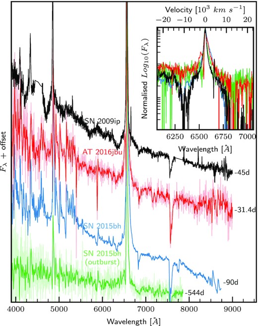
Spectral comparison of SN 2009ip, AT 2016jbu, and SN 2015bh during their respective A events. Also included is the spectrum of SN 2015bh during an apparent LBV outburst in 2013 (Thöne et al. 2017). The inset shows a close-up of H α, normalized to the emission peak to highlight the velocity structure on SN 2009ip. SN 2015bh has been shifted bluewards by 2 Å to match the other H α lines. AT 2016jbu and SN 2015bh have been smoothed with a Gaussian kernel for clarity.
5.1.3 H α comparison
We show a zoom-in on H α in Fig. 20, where the spectra are plotted in order of ‘double-peaked’-ness i.e. according to the level of double-peaked nature of the H α line profile. We arbitrarily define double-peaked-ness as the strength and separation between the two emission peaks (if any) seen in H α. All objects also appear to show an additional high-velocity blue absorption in their Balmer lines (panel B of Fig. 20).13 At intermediate times, ∼3 months after maximum, all transients (excluding SN 2009ip) show clear evidence of strong multicomponent profiles. AT 2016jbu shows the strongest appearance of a double-peaked profile, whereas SN 2009ip shows the least, with weak evidence of some blue excess.
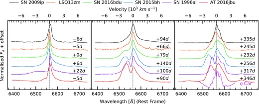
H α spectral comparison between SN 2009ip-like transients. Spectra are plotted after normalizing with respect to the peak of H α, with arbitrary flux offsets for clarity. Spectra were de-reddened using the parameters given in Table A2. Early-time spectra show a Type IIn SNe-like profile with narrow emission. while spectra ∼3 months later show the emergence of a blue and red shoulder in each profile. At late times, H α forms a double-peaked emission profile, aside from in the case of SN 2009ip (although here there is still evidence for a red shoulder component). The difference in line shape is most likely due to inclination, an idea we elaborate on in Section 5. We also show the spectrum of η Car (at ∼+150 yr).
After ∼10 months, all transients show multicomponent profiles in H α. Each transient displays different velocity and FWHM values for their red and blue components. For SN 2009ip, Fraser et al. (2015) note a red component at +500 km s−1 at late times; this shoulder is also seen in H β. We measure the same component at +625 km s−1while fitting for an additional blue component at −510 km s−1. Our fit is illustrated in Fig. 21. In the case of SN 2009ip, this red shoulder only appeared at ∼5.5 months after maximum light, whereas there is evidence of this red shoulder as early as a week after maximum for AT 2016jbu. This is likely due to geometric inclination effects along the line of sight, with SN 2009ip being the most edge on and AT 2016jbu being the more face on. Ejecta-disc models by Kurfürst, Pejcha & Krtička (2020) show this profile shape versus line-of-sight effect.

We include a close-up of the H α profile of η Carin Fig. 20, based on VLT + MUSE observations taken on 2014 November 13. This spectrum was extracted from spaxels with a 14 arcsec radius of η Car after masking nearby stars. η Car displays a multipeaked H α profile similar to what we see in our SN 2009ip-like transients events, albeit at a lower velocity. A similarly shaped profile is also seen in spectra obtained from light echoes of the Great Eruption (GE) (Smith et al. 2018). This resemblance raises the tantalizing possibility that η Car and SN 2009ip-like transients share similar progenitors or progenitor systems.
To date, it is still uncertain what caused the GE in η Car, although commonly discussed scenarios include a major eruption triggered by a merging event in a triple stellar system (Smith et al. 2018), mass transfer from a secondary star during periastron passages (Kashi & Soker 2010), or even a pulsational pair-instability explosion (Woosley, Blinnikov & Heger 2007).
Despite the asymmetric H α emission lines, curiously no other lines show such asymmetry, in particular He i. However, we cannot exclude that this is simply due to lower S/N in these other lines, or that their lower velocities mean that any signs of asymmetry are masked by our moderate instrumental resolution.
6 CONCLUSION
In this paper, we have presented the results of our follow-up campaign for AT 2016jbu consisting of high-cadence photometry up to ∼1.5 yr after maximum light, together with spectra spanning −31 to +420 d covering the UV, optical, and NIR. We also present historical observations over the preceding decade from ground-based observations.
In summary, the salient points of this work are:
AT 2016jbu displays variability in the years prior to maximum light, with outbursts reaching Mr ∼ −11.5 mag, and a double-peaked light curve. The first peak reaches Mr ∼−13.5 mag and the second reaches an SN-like magnitude of Mr ∼−18.26 mag, with both peaks separated by ∼1 month.
AT 2016jbu shows a smooth light curve with a major rebrightening event occurring after the seasonal gap (∼200 d). An increase in He i emission is seen during this time, which may be a sign of increased interaction.
AT 2016jbu appears spectroscopically and photometrically alike to SN 2009ip, SN 2015bh, SN 2016bdu, SN 1996al, SN 2013gc, and SN 2018cnf. However, the increase in brightness at ∼+200 d is unique to AT 2016jbu with respect to our sample of SN 2009ip-like transients. The colour evolution is similar amongst all SN 2009ip-like transients. Colour changes can be linked with the appearance of the red and blue emission components seen in H α.
The H α profiles of each transient show an apparent continuum of asymmetry and we deduce that this may be caused by an geometric inclination effect.
AT 2016jbu and other SN 2009ip-like transients do not exhibit signs of explosive nucleosynthesis at late times such as |$[\mathrm{ O}\, \small{\rm I}]~\lambda \lambda ~6300, 6364$| or |$\mathrm{ Mg}\, \small{\rm I}]~\lambda ~4571$|. On-going CSM interaction may be inhibiting these features and/or obscuring their emitting regions.
AT 2016jbu and the SN 2009ip-like transients are peculiar objects. If they are indeed SNe then their progenitors undergo an unusual and poorly understood series of eruptions in the years prior to core-collapse. If these events are non-terminal and the progenitor star will be revealed in the future, it begs the question what sort of mechanism can produce such an energetic explosion.
In Paper II, we continue the discussion of AT 2016jbu and SN 2009ip-like transients using the data presented here, focusing on the local environment, the progenitor, and modelling of the light curve.
SUPPORTING INFORMATION
AT2016jbu_muiltiband_photometry.txt
Please note: Oxford University Press is not responsible for the content or functionality of any supporting materials supplied by the authors. Any queries (other than missing material) should be directed to the corresponding author for the article.
ACKNOWLEDGEMENTS
SJB acknowledges support from Science Foundation Ireland and the Royal Society (RS-EA/3471). MF is supported by a Royal Society - Science Foundation Ireland University Research Fellowship. TMB was funded by the CONICYT PFCHA / DOCTORADOBECAS CHILE/2017-72180113 and acknowledges their financial support from the Spanish Ministerio de Ciencia e Innovación (MCIN), the Agencia Estatal de Investigación (AEI) 10.13039/501100011033 under the PID2020-115253GA-I00 HOSTFLOWS project, and from Centro Superior de Investigaciones Científicas (CSIC) under the PIE project 20215AT016. KM is funded by the EU H2020 ERC grant no. 758638. TWC acknowledges the EU Funding under Marie Skłodowska-Curie grant H2020-MSCA-IF-2018-842471, and thanks to Thomas Krühler for GROND data reduction. MN is supported by a Royal Astronomical Society Research Fellowship. BJS is supported by NSF grants AST-1908952, AST-1920392, AST-1911074, and NASA award 80NSSC19K1717. MS is supported by generous grants from Villum FONDEN (13261, 28021) and by a project grant (8021-00170B) from the Independent Research Fund Denmark. LH acknowledges support for Watcher from Science Foundation Ireland grant 07/RFP/PHYF295. Time domain research by DJS is supported by NSF grants AST-1821987, 1813466, and 1908972, and by the Heising-Simons Foundation under grant #2020-1864. NER acknowledges support from MIUR, PRIN 2017 (grant 20179ZF5KS). LG acknowledges financial support from the Spanish Ministry of Science, Innovation and Universities (MICIU) under the 2019 Ramón y Cajal program RYC2019-027683 and from the Spanish MICIU project PID2020-115253GA-I00. Support for TW-SH was provided by NASA through the NASA Hubble Fellowship grant HST-HF2-51458.001-A awarded by the Space Telescope Science Institute, which is operated by the Association of Universities for Research in Astronomy, Inc., for NASA, under contract NAS5-26555. Support for JLP is provided in part by ANID through the Fondecyt regular grant 1191038 and through the Millennium Science Initiative grant ICN12_009, awarded to The Millennium Institute of Astrophysics, MAS. DAH and DH are supported by AST-1911151, AST19-11225, and NASA Swift grant 80NSSC19K1639. GP acknowledge support by the Ministry of Economy, Development, and Tourism’s Millennium Science Initiative through grant IC120009, awarded to The Millennium Institute of Astrophysics, MAS. LT acknowledges support from MIUR (PRIN 2017 grant 20179ZF5KS). HK was funded by the Academy of Finland projects 324504 and 328898.
This research used astropy,14 a community-developed core Python package for Astronomy (Astropy Collaboration 2013; Price-Whelan et al. 2018). This research used data provided by Astrometry.net.15 This research has used the NASA/IPAC Extragalactic Database (NED), which is operated by the Jet Propulsion Laboratory, California Institute of Technology, under contract with the National Aeronautics and Space Administration. We acknowledge the use of public data from the Swift data archive. This work used data supplied by the UK Swift Science Data Centre at the University of Leicester. We acknowledge Telescope Access Program (TAP) funded by the NAOC, CAS, and the Special Fund for Astronomy from the Ministry of Finance. This work was partially supported from Polish NCN grants: Harmonia No. 2018/30/M/ST9/00311 and Daina No. 2017/27/L/ST9/03221. Parts of this research were supported by the Australian Research Council Centre of Excellence for All-Sky Astrophysics in 3 Dimensions (ASTRO 3D), through project number CE170100013. This work is based in part on observations made with the Spitzer Space Telescope, which was operated by the Jet Propulsion Laboratory, California Institute of Technology under a contract with NASA. Support for this work was provided by NASA through an award issued by JPL/Caltech. This work used v2.2.1 of the Binary Population and Spectral Synthesis (BPASS) models as described in Eldridge et al. (2017) and Stanway & Eldridge (2018).
This publication uses data products from the Two Micron All-Sky Survey, which is a joint project of the University of Massachusetts and the Infrared Processing and Analysis Center/California Institute of Technology, funded by the National Aeronautics and Space Administration and the National Science Foundation. This paper includes data gathered with the 6.5 meter Magellan Telescopes located at Las Campanas Observatory, Chile. This publication uses data products from the Wide-field Infrared Survey Explorer, which is a joint project of the University of California, Los Angeles, and the Jet Propulsion Laboratory/California Institute of Technology, funded by the National Aeronautics and Space Administration. This research is based on observations made with the NASA/ESA Hubble Space Telescope obtained from the Space Telescope Science Institute, which is operated by the Association of Universities for Research in Astronomy, Inc., under NASA contract NAS 5-26555. These observations are associated with program 15645. Observations were also obtained from the Hubble Legacy Archive, which is a collaboration between the Space Telescope Science Institute (STScI/NASA), the Space Telescope European Coordinating Facility (ST-ECF/ESAC/ESA) and the Canadian Astronomy Data Centre (CADC/NRC/CSA). This work used data from the Las Cumbres Observatory network. We thank the Las Cumbres Observatory and its staff for its continuing support of the ASAS-SN project. ASAS-SN is supported by the Gordon and Betty Moore Foundation through grant GBMF5490 to the Ohio State University, and NSF grants AST-1515927 and AST-1908570. Development of ASAS-SN has been supported by NSF grant AST-0908816, the Mt. Cuba Astronomical Foundation, the Center for Cosmology and AstroParticle Physics at the Ohio State University, the Chinese Academy of Sciences South America Center for Astronomy (CAS- SACA), and the Villum Foundation. This research has used the SVO Filter Profile Service16 supported from the Spanish MINECO through grant AYA2017-84089. We acknowledge ESA Gaia, DPAC and the Photometric Science Alerts Team.17 This project used data obtained with the Dark Energy Camera (DECam), which was constructed by the Dark Energy Survey (DES) collaborating institutions: Argonne National Lab, University of California Santa Cruz, University of Cambridge, Centro de Investigaciones Energeticas, Medioambientales y Tecnologicas-Madrid, University of Chicago, University College London, DES-Brazil consortium, University of Edinburgh, ETH-Zurich, University of Illinois at Urbana-Champaign, Institut de Ciencies de l’Espai, Institut de Fisica d’Altes Energies, Lawrence Berkeley National Lab, Ludwig-Maximilians Universitat, University of Michigan, National Optical Astronomy Observatory, University of Nottingham, Ohio State University, University of Pennsylvania, University of Portsmouth, SLAC National Lab, Stanford University, University of Sussex, and Texas A&M University. Funding for DES, including DECam, has been provided by the U.S. Department of Energy, National Science Foundation, Ministry of Education and Science (Spain), Science and Technology Facilities Council (UK), Higher Education Funding Council (England), National Center for Supercomputing Applications, Kavli Institute for Cosmological Physics, Financiadora de Estudos e Projetos, Fundação Carlos Chagas Filho de Amparo a Pesquisa, Conselho Nacional de Desenvolvimento Científico e Tecnológico and the Ministério da Ciência e Tecnologia (Brazil), the German Research Foundation-sponsored cluster of excellence ‘Origin and Structure of the Universe’ and the DES collaborating institutions. Based on observations obtained with XMM–Newton, an ESA science mission with instruments and contributions directly funded by ESA Member States and NASA.Based on observations obtained at the international Gemini Observatory (GS-2016B-Q-22), a program of NSF’s NOIRLab, which is managed by the Association of Universities for Research in Astronomy (AURA) under a cooperative agreement with the National Science Foundation. on behalf of the Gemini Observatory partnership: the National Science Foundation (United States), National Research Council (Canada), Agencia Nacional de Investigación y Desarrollo (Chile), Ministerio de Ciencia, Tecnología e Innovación (Argentina), Ministério da Ciência, Tecnologia, Inovações e Comunicações (Brazil), and Korea Astronomy and Space Science Institute (Republic of Korea). This paper includes data gathered with the Nordic Optical Telescope (PI Stritzinger) at the Observatorio del Roque de los Muchachos, La Palma, Spain. We thank Norbert Schartel for rapid approval and scheduling of ToO observations (ObsID 0794580101). Based on observations collected at the European Organisation for Astronomical Research in the Southern Hemisphere under ESO programmes 1103.D-0328, 1103.D-0328, 199.D-0143, 197.D-1075, 191.D-0935 (PESSTO, ePESSTO and ePESSTO +). In addition, data taken under ESO programmes 098.A-9099, 0104.A-9099, 0100.D-0865, 098.D-0692, 100.D-0341, and 0103.D-0139(A) are presented here. Based in part on data acquired at the ANU 2.3m Telescope at Siding Spring Observatory. We acknowledge the traditional owners of the land on which the telescope stands, the Gamilaraay people, and pay our respects to elders past, present, and emerging. Part of the funding for GROND (both hardware as well as personnel) was generously granted from the Leibniz-Prize to Prof. G. Hasinger (DFG grant HA 1850/28-1). The OGLE project has received funding from the National Science Centre, Poland, grant MAESTRO 2014/14/A/ST9/00121 to AU. LCO data have been obtained via OPTICON proposals and was obtained as part of the Global Supernova Project. The OPTICON project has received funding from the European Union’s Horizon 2020 research and innovation programme under grant agreement No 730890.
DATA AVAILABILITY
The spectroscopic data underlying this article are available in the Weizmann Interactive Supernova Data Repository at https://wiserep.weizmann.ac.il/. The photometric data underlying this article are available in the article and in its online supplementary material.
Footnotes
iraf is distributed by the National Optical Astronomy Observatory, which is operated by the Association of Universities for Research in Astronomy (AURA) under cooperative agreement with the National Science Foundation.
referred to as ‘flickering’ in Kilpatrick et al. (2018).
The spectroscopic data for SN 1996al only begin at 22 d past Event B, when we can already see the emergence of a broad blue component.
REFERENCES
APPENDIX A: PHOTOMETRY TABLES
Sample of full photometry table for AT 2016jbu. All measurements were carried out using AutoPhoT. Phase is with respect to V-band maximum of Event B. Limiting magnitudes listed where AT 2016jbu could not be detected, and 1σ errors are given in parentheses. UBVRIJHK filters are in Vegamags, ugriz are in AB magnitudes. Full photometry table available online.
| Date | MJD | Phase (d) | u | g | r | i | z | U | B | V | R | I | J | H | K | Instrument |
|---|---|---|---|---|---|---|---|---|---|---|---|---|---|---|---|---|
| 1999-12-26 | 51538.5 | −6245.9 | – | – | – | – | – | – | >22.63 | – | – | – | – | – | – | WFI |
| 2000-02-17 | 51591.0 | −6193.4 | – | – | – | – | – | – | >22.66 | >21.94 | >22.80 | – | – | – | – | WFI |
| 2000-04-05 | 51639.0 | −6145.4 | – | – | – | – | – | – | – | – | >23.33 | – | – | – | – | WFI |
| 2001-02-04 | 51944.0 | −5840.4 | – | – | – | – | – | – | – | >22.37 | >23.20 | – | – | – | – | WFI |
| 2005-03-13 | 53442.0 | −4342.4 | – | – | – | – | – | – | – | >22.54 | – | – | – | – | – | CTIO + MOSAIC |
| 2005-03-14 | 53443.0 | −4341.4 | – | – | – | – | – | – | – | >22.59 | >20.50 | – | – | – | – | CTIO + MOSAIC |
| 2006-01-29 | 53764.0 | −4020.4 | – | – | – | – | – | – | – | >23.19 | – | – | – | – | – | WFI |
| 2006-01-29 | 53764.5 | −4019.9 | – | – | – | – | – | – | – | >23.23 | – | – | – | – | – | WFI |
| 2006-01-30 | 53765.0 | −4019.4 | – | – | – | – | – | – | >24.36 | – | – | – | – | – | – | WFI |
| 2006-10-06 | 54014.0 | −3770.4 | – | – | – | – | – | – | – | – | >16.36 | – | – | – | – | Prompt |
Properties of SN 2009ip-like transient events. Values reported are used consistently throughout this work. The time of peak is with respect to the Event B maximum. Where quoted, 56Ni masses are upper limits.
| Transient | z | AV [mag] a | μ [mag] | Peak (MJD) b | 56Ni [M⊙] | Reference |
|---|---|---|---|---|---|---|
| AT 2016jbu | 0.00489 | 0.556 | 31.60 | 57784 | ≤0.016 | This paper; Paper II; Cartier et al. (2017) |
| SN 2009ip | 0.00572 | 0.054 | 31.55 | 56203 | ≤0.020 | Fraser et al. (2013), Pastorello et al. (2013) |
| SN 2013gc | 0.00340 | 1.253 | 30.46 | 56544 | ≤0.004 | Reguitti et al. (2019) |
| SN 2015bh | 0.00644 | 0.062 | 32.40 | 57166 | ≤0.003 | Thöne et al. (2017), Elias-Rosa et al. (2016) |
| SN 2016bdu | 0.0173 | 0.041 | 34.37 | 57541 | – | Pastorello et al. (2018) |
| LSQ13zm | 0.029 | 0.052 | 35.43 | 56406 | – | Tartaglia et al. (2016) |
| SN 1996al | 0.0065 | 0.032 | 31.80 | 50265 | – | Benetti et al. (2016) |
| SN 2018cnf | 0.02376 | 0.118 | 34.99 | 58293 | – | Pastorello et al. (2019) |
Notes.aGalactic extinction only. If AV not mentioned in reference, we take values from NED.
bWith respect to Event B maximum light in V band.
