


ABSTRACT
In this paper, wavelet analysis is used to study the spectral-timing properties of MAXI J1535–571 observed by the Hard X-ray Modulation Telescope (Insight-HXMT). Low-frequency quasi-periodic oscillations (QPOs) are detected in nine observations. Based on wavelet analysis, the time intervals with QPOs and non-QPOs are isolated, and the corresponding spectra with QPOs and non-QPOs are analysed. We find that the spectra with QPOs (hereafter QPO spectra) are softer than those without QPOs (hereafter non-QPO spectra) in the hard intermediate state (HIMS), while in the soft intermediate state (SIMS), the QPO spectra are slightly harder. The disc temperature of the QPO regime is slightly lower during the HIMS, but becomes higher during the SIMS. The cutoff energies of QPO spectra and non-QPO spectra do not show significant differences. The flux ratio of the disc to total flux is higher for the time intervals with non-QPOs than that in the QPO regime. We propose that these differences in the spectral properties between QPO and non-QPO regimes could be explained through the scenario of Lense–Thirring precession, and the reversal of the QPO/non-QPO behaviour between the HIMS and SIMS may be associated with the appearance/disappearance of a type-B QPO, which might originate in the precession of the jet.
1 INTRODUCTION
Black hole (BH) transients are briefly detected during their outbursts. They are worthy of study in the X-ray because of the interesting variation in their timing and spectral properties (Kara et al. 2019; You et al. 2021). Typically, the spectral states of a BH transient in an outburst evolve through a hard state (HS), hard/soft intermediate states (HIMS/SIMS), a soft state (SS), intermediate states again, and finally back to a HS (Remillard & McClintock 2006; Belloni 2010).
Low-frequency quasi-periodic oscillations (LFQPOs), with their centroid frequencies ranging from 0.01 to 30 Hz, are commonly observed in stellar-mass BHs (Motta et al. 2015; Motta 2016; Ingram & Motta 2019; Ma et al. 2021). Three types (A, B, C) of LFQPOs are identified, based on their power spectrum features (Remillard et al. 2002; Casella, Belloni & Stella 2005; Ingram & Motta 2019; Xiao et al. 2019; Zhang et al. 2021). Studies reveal that relationships exist between LFQPO types and spectral states: type-A/B QPOs are normally seen in the SIMS (Belloni et al. 2020; García et al. 2021), while type-C QPOs can be found in the HS, HIMS and SS (Nandi et al. 2012; Muñoz Darias et al. 2014; de Ruiter et al. 2019).
The origin and properties of LFQPOs are still under debate. A number of models have been proposed to explain type-C QPOs (e.g. Molteni, Sponholz & Chakrabarti 1996; Stella, Vietri & Morsink 1999; Tagger & Pellat 1999; Wagoner 1999; Kato 2001; Schnittman, Homan & Miller 2006; Chakrabarti et al. 2008; Ingram, Done & Fragile 2009; Cabanac et al. 2010). Many of these theories are based on Lense–Thirring precession and generally can be categorized as geometrical and intrinsic models (You, Bursa & Życki 2018; You et al. 2020; Ingram & Motta 2019). Observations have shown that the generation of type-C QPOs is related to geometry and/or precession (e.g. Ingram & Done 2012; Motta et al. 2015; Axelsson & Done 2016), but no clear conclusion regarding Lense–Thirring precession has been drawn (Ingram & Motta 2019). For type-B and type-A QPOs, the physical origin is even less clear, except that type-B QPOs may be connected to jets (Fender, Homan & Belloni 2009; Motta et al. 2015; Russell et al. 2020).
In recent decades, the sudden appearance or disappearance of all three types of QPOs has been discovered in several sources (e.g. Miyamoto et al. 1991; Nespoli et al. 2003; Huang et al. 2018; Xu et al. 2019; Sriram, Harikrishna & Choi 2021). These fast transitions are sometimes associated with type variations, mostly a type-A/B transition (Nespoli et al. 2003; Sriram, Rao & Choi 2012, 2013, 2016), but type-B/C (Homan et al. 2020) or even type-C/A (Bogensberger et al. 2020) transitions are also reported. Many of these QPO timing studies are based on the dynamical power density spectra (PDS) technique, with intervals of a few tens of seconds (e.g. Zhang et al. 2021; Sriram et al. 2021), and thus have a limit on the time resolution of tens of seconds. Wavelet analysis, on the other hand, can provide accurate time–frequency-space information with sufficiently small time intervals, and thus can be used to study the detailed variations of the periodic or quasi-periodic signals over time (Ding et al. 2021).
The outburst of the Galactic BH transient MAXI J1535–571 was first detected during 2017 September, simultaneously by the Gas Slit Camera of the Monitor of All-sky X-ray Image (MAXI/GSC; Negoro et al. 2017) and the Burst Alert Telescope of Swift (Swift/BAT; Kennea et al. 2017), and subsequently by radio (Russell et al. 2017; Tetarenko et al. 2017), submillimetre (Tetarenko et al. 2017), near-infrared (Dinçer 2017) and optical (Scaringi & Students 2017) observations. The state transitions (Nakahira et al. 2017; Palmer, Krimm & Team 2017; Shidatsu et al. 2017; Tao et al. 2018; Russell et al. 2019; Cúneo et al. 2020) and LFQPOs (Gendreau et al. 2017; Mereminskiy & Grebenev 2017; Bhargava et al. 2019; Chatterjee et al. 2020; Vincentelli et al. 2021) of this source have been discussed. A Hard X-ray Modulation Telescope (HXMT, also dubbed as Insight-HXMT) observation was also performed in 2017 September, and its state transitions and QPOs have been studied (Huang et al. 2018; Kong et al. 2020).
In this paper, wavelet analysis is utilized to study the 2017 outburst of MAXI J1535–571 with Insight-HXMT data. The observations and data reductions are introduced in Section 2. Section 3 gives the details of the data analysis, including the wavelet methods, data separation with QPOs and non-QPOs, and spectral analysis. In Section 4, the distinctions between QPO spectra and non-QPO spectra are discussed. Finally, in Section 5 we summarize the results and present the implications.
2 OBSERVATIONS AND DATA REDUCTION
Insight-HXMT, the first Chinese X-ray satellite, covers a broad energy band. It contains three telescopes with different energy ranges: the High-Energy X-ray telescope (HE) has 18 NaI/CsI detectors covering the range 20–250 keV with a geometrical area of ∼5100 cm2; the Medium-Energy X-ray telescope (ME) covers 5–30 keV with 1728 Si-PIN detectors, with a collecting area of 952 cm2; and the swept charge device is used in the Low Energy X-ray telescope (LE), covering the energy range 1–15 keV with a total collecting area of 384 cm2 (Zhang et al. 2020). The typical fields of view (FoVs) are 1.1° × 5.7°, 1° × 4° and 1.6° × 6° for HE, ME and LE, respectively (Zhang et al. 2020).
The MAXI J1535–571 observations were performed by Insight-HXMT from 2017 September 6 to 18. A gap is apparent in the downloaded data between September 7 and 12 due to the X9.3 solar flare. These observational details are discussed in Kong et al. (2020) and Huang et al. (2018). After the outburst, 10 more observations were triggered sporadically in 2018 February, and are also included in our data processing.
The Insight-HXMT Data Analysis Software (hxmtdas) version 2.04 is used to analyse the data. The pointing offset angle is smaller than 0.°04; the elevation angle is greater than 10°; the geomagnetic cutoff rigidity is larger than 8°; and data within 300 s of the South Atlantic Anomaly (SAA) passage are not used. The light curves are made by the hxmtdas tasks helcgen, melcgen and lelcgen with 0.01-s time bins. The official tools hebkgmap, mebkgmap and lebkgmap of version 2.0.12 are adopted for both the spectrum and the light-curve background estimation.
3 METHODS
3.1 Wavelet analysis
Different ‘mother’ wavelets and wavelet parameters m will affect the final results. As indicated by Del Moortel, Munday & Hood (2004), the Morlet wavelet or a larger value of m makes the frequency resolution better, while the Paul wavelet or a smaller value of m gives a better time resolution. Because both frequency resolution and time resolution are important in our study, the Morlet wavelet with m = 6 has been taken to achieve a compromise, and to satisfy the admissibility condition (Farge 1992). As a comparison, the Paul wavelet with m = 6 and a dynamical PDS with a time resolution of 1 s were also tested, and both provide similar peak numbers and locations around the QPO frequency (see Appendix A for a comparison of the dynamical power spectrum and wavelet analysis). The Paul wavelet, however, performs poorly in frequency resolution, and the confidence areas in time are quite narrow, which may affect the fitting results of the QPO spectra, while for the dynamical PDS, the windowed Fourier transform utilized is inaccurate and inefficient (Kaiser 2011).
The determination of significance levels was also discussed in Torrence & Compo (1998). A white- or red-noise background spectrum should be appropriately chosen, and the actual spectrum can be compared with this randomly distributed background. In our case, the lag-1 autoregressive [AR(1)] is used for red-noise calculation. At each point (n, s) in the local wavelet power spectrum, the degree of freedom is two. Based on the chi-squared distribution, if a power in the wavelet power spectrum is above the 95 per cent confidence level (i.e. significant at the 5 per cent level) compared with the background spectrum, then it can be considered as a true signal.
Because smooth, continuous variations in time series can improve accuracy, and giant time intervals exist in nearly all light curves because of the good time intervals (GTIs), we separate the light-curve data if the adjacent time difference is greater than 0.1 s, which is 10 times the time bin size. As a consequence, HE and ME light curves are normally split into ∼5 time ranges, while LE light curves contain 1 or 2 separated data ranges, which are basically the same as the GTI segments (see Appendix B for detailed GTI information on three instruments).
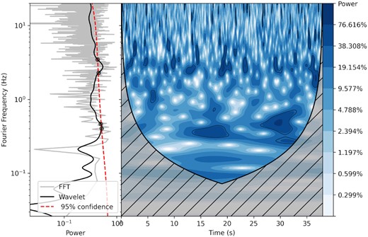
Fig. 1 gives an example plot of the wavelet analysis. The time series used here is that of the separated HE light curve of observation P011453500144 (hereafter, the observation ID will be written as the last three digits for short, i.e. Obs 144) with the background subtracted. The global wavelet power spectrum (black line) is presented in the left-hand plot, along with the PDS results (grey line) for comparison. The 95 per cent confidence level for the global wavelet spectrum is also presented, as the red dashed line. The local wavelet power spectrum is shown on the right-hand side. As the power increases, the plot colour changes from white to dark blue. Regions above the 95 per cent confidence level are enclosed with the black contour. Cross-hatched regions at the bottom indicate the cone of influence area, which is caused by the temporary padding (with zeros) at the end of the time series before performing the wavelet transform. The padding enables edge time series to be calculated with wavelet analysis, but also reduces the credibility of that time series. Thus we weighted this area by a factor of 0.1 when plotting. In this figure, a peak is clearly visible in the PDS, global wavelet spectrum and local wavelet powers. This demonstrates the reliability of the wavelet algorithm and also provides the basis for the next step.

Global wavelet spectra (left-hand side, black line) and contour plot (right-hand side) of wavelet results for Obs 144. In the left-hand window, the PDS result is shown by the grey line, the 95 per cent confidence level is plotted with the red dashed line, and the cross points of the global wavelet spectra and 95 per cent confidence level are presented with dark circles. In the contour plot, the black line encloses the area where signals exceed the 95 per cent confidence level, and the grey hashed area refers to the cone of influence.
The wavelet results are discrete data, and the step of the logarithmic period is 0.015, which gives a step size of ∼0.3 Hz around 9 Hz and of ∼0.085 Hz around 2.5 Hz, which results in relatively reliable data. Details of the data separation are discussed in the next subsection. The difference of the peaks between GTIs of the same observation is normally less than 0.3 Hz. Here we weight the global wavelet spectra by time and sum them together for each observation. The QPO information and the mean count rate of each observation are shown in Table 1 for comparison with previous studies. Because the advantage of wavelet analysis is that it provides detailed time–frequency information, and the global wavelet spectrum is not as efficient as PDS in the power spectrum analysis (Liu, San Liang & Weisberg 2007; Bravo et al. 2014), only the central frequency and its full width at half-maximum (FWHM) are provided. The QPO centroid frequency increases gradually from ∼2.5 to ∼9 Hz, except for Obs 301. Kong et al. (2020) and Huang et al. (2018) reported the QPO centroid frequencies derived from the energy range of 27.4–31.2 and 6–38 keV, respectively. Compared with our ME results from 10–27 keV, the frequencies are consistent. Our LE (2–10 keV) QPO centroid frequencies are basically the same as the Neutron star Interior Composition Explorer (NICER; 0.2–10 keV) and Swift/XRT (0.3–10 keV) results, both reported by Stiele & Kong (2018); that is, the QPO frequency first decreased from ∼2.5 to 2 Hz, then increased to 3 Hz at around Obs 601, and finally increased to 9 Hz at Obs 901.
The QPO centroid frequency, FWHM, and mean count rate of each observation. The observation IDs are the last three digits of P011453500XXX.
| Obs | Start time (s) | LE | ME | HE | State | ||||||
|---|---|---|---|---|---|---|---|---|---|---|---|
| QPO υ (Hz) | FWHM | Count rate | QPO υ (Hz) | FWHM | Count rate | QPO υ (Hz) | FWHM | Count rate | |||
| 144 | 2017-09-12T10:38:15 | 2.61 ± 0.01 | 0.79 | 1168.09 | 2.59 ± 0.01 | 0.83 | 358.52 | 2.56 ± 0.01 | 0.76 | 533.00 | HIMS |
| 145 | 2017-09-12T13:58:12 | 2.56 ± 0.01 | 0.87 | 1188.39 | 2.61 ± 0.01 | 0.90 | 364.35 | 2.61 ± 0.01 | 0.87 | 548.24 | HIMS |
| 301 | 2017-09-15T04:48:00 | 2.14 ± 0.01 | 0.66 | 1309.80 | 2.09 ± 0.01 | 0.67 | 448.36 | 2.02 ± 0.01 | 0.62 | 684.73 | HIMS |
| 401 | 2017-09-16T06:15:29 | 2.79 ± 0.01 | 0.84 | 1482.88 | 2.79 ± 0.01 | 0.87 | 440.11 | 2.79 ± 0.01 | 0.84 | 607.65 | HIMS |
| 501 | 2017-09-17T06:07:38 | 3.36 ± 0.01 | 1.01 | 1713.80 | 3.40 ± 0.01 | 1.08 | 449.40 | 3.40 ± 0.01 | 1.06 | 576.74 | HIMS |
| 601 | 2017-09-18T02:48:54 | 3.32 ± 0.01 | 1.02 | 1759.82 | 3.38 ± 0.01 | 1.07 | 469.73 | 3.35 ± 0.01 | 1.07 | 615.66 | HIMS |
| 901 | 2017-09-21T02:26:26 | 8.59 ± 0.04 | 2.42 | 2675.21 | 9.07 ± 0.01 | 2.85 | 361.92 | 9.28 ± 0.02 | 2.88 | 371.80 | SIMS |
| 902 | 2017-09-21T06:00:41 | 8.45 ± 0.16 | 2.71 | 2685.83 | 9.22 ± 0.02 | 2.89 | 351.46 | 9.32 ± 0.02 | 2.91 | 375.27 | SIMS |
| 903 | 2017-09-21T09:21:07 | 7.59 ± 0.08 | 2.58 | 2626.91 | 8.21 ± 0.01 | 2.97 | 384.63 | 9.07 ± 0.03 | 2.90 | 405.24 | SIMS |
3.2 Time split and spectral analysis
Based on the wavelet results, we separate data by the 95 per cent confidence level. Because the peak area on the local wavelet spectrum of Fig. 1 is quite dense because of the long time range, a ∼40-s time segment result is shown in Fig. 2, to elaborate the details of the selection of the time period. Once the peak frequency of the global wavelet power curve is confirmed, the 95 per cent confidence interval of the frequency can be chosen, that is, the intersection range between the global wavelet power curve and the 95 per cent confidence red line near the peak. Then, if any point in the local wavelet plot within this frequency interval is greater than the 95 per cent confidence level (the points within the area enclosed by the black contour in Fig. 2), the point is selected as the QPO time range. Using this method, we select out all the QPO time ranges in each observation, and then the hxmtscreen tool in hxmtdas is used to create a new FITS file that only contains these segments, to replace the original screened event FITS file. Then the normal hxmtdas spectrum generation pipeline steps are executed to generate a new spectrum that just contains the QPO time-segment information. All the remaining time ranges are below the 95 per cent confidence level. Mathematically speaking, they cannot be guaranteed as QPO-excluded segments. However, they will be referred to as non-QPO segments from now on, for the sake of convenience. Similarly, the non-QPO time ranges are used for non-QPO spectrum generation. Finally, for each observation, we have three spectra: one for time-averaged regime, one for QPO-included regime, and one for QPO-excluded regime.
Time selection diagram for a ∼40-s wavelet result. Elements in the plot are basically the same as in Fig. 1.
Before further considering the separated spectrum, we make an analysis of the separated time segments, and the rms results are shown in Fig. 3, including the rms of QPO segments in 0.1–32 Hz and 2–4 Hz, and the rms of the whole-time segments in 0.1–32 Hz and 2–4 Hz. Because the QPO time ranges are quite narrow, typically from about a second to a few seconds, a 2-s data interval is chosen for PDS production for both QPO segments and the whole time, to ensure consistency. As a consequence, rms values in the QPO regime and time-averaged regime are obtained for Obs 144–501, and the rms values versus hardness are shown in Fig. 3. Obviously, the QPO regime has larger error bars, because the number of averaged time segments is smaller compared with the time-averaged regime. A positive correlation between the rms values and hardness can be noted in the time-averaged regime (e.g. Spearman rank correlation r = 0.956 and p = 0.01 for 2–4 Hz). However, in the case of the QPO regime, this relationship is not clear. If this change is not caused by error bars, then the positive correlation is not related to the appearance of QPOs. The rms value during the QPO regime is much larger than in the time-averaged scenario, both for 0.1–32 Hz and for 2–4 Hz. The averaged rms of the five points in the QPO regime increased by |$\sim15{{\%}}$| in 0.1–32 Hz, and |$\sim50{{\%}}$| in 2–4 Hz, compared with the time-averaged regime. We also calculate the rms values in 0.1–2 Hz and 4–32 Hz, and find that they remain almost unchanged between the two regimes (changing by |$\sim-6{{\%}}$| and 0.2 per cent for 0.1–2 Hz and 4–32 Hz, respectively). The above results may indicate that, first of all, the light curves in the QPO regime are indeed different from the time-averaged data. Secondly, this change is concentrated mainly around the QPO frequency, rather than in other frequency bands.
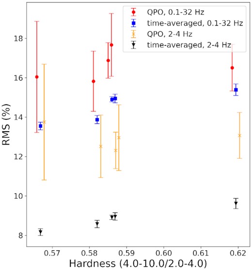
Hardness–rms diagram, where hardness is the ratio of the mean count rates of 4.0–12.0 keV to 2.0–4.0 keV. The red circles, blue squares, orange crosses and black inverted triangles represent rms values in the QPO regime in 0.1–32 Hz, the time-averaged regime in 0.1–32 Hz, the QPO regime in 2–4 Hz, and the time-averaged regime in 2–4 Hz, respectively. Only Obs 144–501 are plotted for both QPO and time-averaged regimes. The QPO regimes have large error bars, and are shifted a little to the left (0.1–32 Hz) and right (2–4 Hz) to avoid overlapping.
Fig. 4 also gives the evolution of hardness (4.0–12.0 keV to 2.0–4.0 keV) with time (top panel), and the QPO frequency–hardness diagram (bottom panel). The hardness basically shows a decreasing trend with time, except for Obs 301, which also shows a different trend in the evolution of QPO frequency (see Table 1). In addition, the diagram of QPO frequency and hardness shows an anticorrelation, with the Spearman rank correlation r = −0.881 and p = 0.001. The top panel of Fig. 4 also indicates that a difference exists between the QPO regime and the non-QPO regime, and the hardness of the QPO regime is greater than that of the non-QPO one.

Top panel: The hardness evolution with time, where hardness is defined as the ratio of mean count rates of 4.0–12.0 keV to 2.0–4.0 keV, and the horizontal axis is the time since Obs 144 in days. Hardnesses in time-averaged (black circles), QPO (red crosses) and non-QPO (blue triangles) regimes are plotted. Bottom panel: Centroid QPO frequency–hardness diagram, where hardness has the same definition as in the top panel, except that only time-averaged results are shown, and here frequency is the centroid QPO frequency of LE light curves.
Next, we use the xspec v12.12.0 software package (Arnaud 1996) to fit these spectra. The spectra are grouped to have at least 30 counts in each energy bin. Xu et al. (2018) reported a strong iron line in this source in the HS, which was also reported with the Insight-HXMT in the HS (Kong et al. 2020). However, when the source entered the HIMS and SIMS, this Fe Kα line was hardly seen (also see Kong et al. 2020). Thus, similar to in the previous work (i.e. Kong et al. 2020), we consider const*tbabs*(diskbb + cutoffpl) as the model in the spectral fitting, and the results are shown in Table 2. During the SIMS (i.e. Obs 901–903), the values of Ecut are much higher than 100 keV, with large uncertainties, resulting in no physical meaning, so we fix them at 400 keV. Fig. 5 presents examples of the spectral fitting results. The top panel shows spectra of Obs 144 in the HIMS, while the bottom panel shows those of Obs 901 in the SIMS. A systematic error of 2 per cent for LE/ME/HE was added. In this study, the uncertainty of the best-fitting parameters corresponds to the 90 per cent confidence level. The energy bands adopted for analysis are 2–10 keV (LE), 10–27 keV (ME) and 27–100 keV (HE).
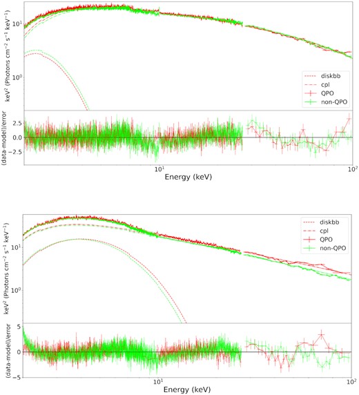
A combo plot of QPO (red) and non-QPO (green) fitting spectra for Obs 144 (top) and Obs 901 (bottom). The energy band is from 2 to 100 keV, with 2–10 keV for LE, 10–27 keV for ME, and 27–100 keV for HE. Model: const*tbabs*(diskbb + cutoffpl), with NH fixed to |$3.8\times 10^{22} \rm \ cm^{-2}$|.
Spectral fitting parameters. The model used here is const*tbabs*(diskbb + cutoffpl), with NH fixed to |$3.8\times 10^{22} \rm \ cm^{-2}$|. A systematic error of 2% is adopted when calculating χ2. The exposure time after data reduction is listed in the last column.
| Obs | Tin | diskbb norm | Γ | Ecut | cutoffpl norm | χ2/d.o.f. | Exposure |
|---|---|---|---|---|---|---|---|
| (keV) | (105) | (keV) | (s) | ||||
| LE/ME/HE | |||||||
| Time-averaged | |||||||
| 144 | 0.38 ± 0.01 | |$2.56 _{- 0.54 }^{+ 0.73 }$| | 2.27 ± 0.01 | |$68.83 _{- 2.79 }^{+ 3.02 }$| | |$37.60 _{- 0.80 }^{+ 0.80 }$| | 1160.32 / 1275 | 1137 / 2168 / 1684 |
| 145 | 0.37 ± 0.01 | |$3.08 _{- 0.56 }^{+ 0.73 }$| | 2.29 ± 0.01 | |$69.80 _{- 1.85 }^{+ 1.94 }$| | |$39.63 _{- 0.59 }^{+ 0.59 }$| | 1159.93 / 1275 | 3181 / 8202 / 9329 |
| 301 | 0.34 ± 0.01 | |$5.89 _{- 1.42 }^{+ 2.00 }$| | 2.16 ± 0.01 | |$53.12 _{- 1.63 }^{+ 1.71 }$| | |$37.49 _{- 0.75 }^{+ 0.75 }$| | 1163.08 / 1275 | 599 / 3380 / 1636 |
| 401 | 0.35 ± 0.01 | |$4.51 _{- 1.09 }^{+ 1.55 }$| | 2.32 ± 0.01 | |$63.69 _{- 1.83 }^{+ 1.93 }$| | |$52.38 _{- 0.93 }^{+ 0.92 }$| | 1070.94 / 1275 | 1017 / 3829 / 4870 |
| 501 | 0.35 ± 0.02 | |$4.24 _{- 1.36 }^{+ 2.27 }$| | 2.44 ± 0.01 | |$73.04 _{- 2.43 }^{+ 2.58 }$| | |$71.91 _{- 1.27 }^{+ 1.26 }$| | 1167.57 / 1275 | 1017 / 3979 / 5079 |
| 601 | 0.36 ± 0.02 | |$4.28 _{- 1.46 }^{+ 2.58 }$| | 2.41 ± 0.02 | |$68.30 _{- 3.62 }^{+ 3.98 }$| | |$71.37 _{- 1.71 }^{+ 1.70 }$| | 1113.24 / 1275 | 479 / 3194 / 714 |
| 901 | 1.18 ± 0.01 | *1.80 ± 0.08 | 2.87 ± 0.01 | †400.00 | |$144.77_{- 2.34 }^{+ 2.37 }$| | 1184.82 / 1276 | 1676 / 2967 / 2467 |
| 902 | 1.17 ± 0.01 | *1.91 ± 0.08 | 2.87 ± 0.01 | †400.00 | |$144.22_{- 2.33 }^{+ 2.37 }$| | 1210.98 / 1276 | 1820 / 2780 / 3697 |
| 903 | 1.17 ± 0.01 | *1.52 ± 0.09 | 2.84 ± 0.01 | †400.00 | |$143.93_{- 2.47 }^{+ 2.51 }$| | 1119.86 / 1276 | 1116 / 2471 / 366 |
| Non-QPO | |||||||
| 144 | 0.39 ± 0.01 | |$2.32 _{- 0.48 }^{+ 0.66 }$| | 2.24 ± 0.01 | |$67.18 _{- 2.91 }^{+ 3.16 }$| | |$35.79 _{- 0.84 }^{+ 0.85 }$| | 1166.41 / 1275 | 913 / 1702 / 1250 |
| 145 | 0.38 ± 0.01 | |$2.48 _{- 0.42 }^{+ 0.54 }$| | 2.26 ± 0.01 | |$68.24 _{- 1.89 }^{+ 1.99 }$| | |$37.72 _{- 0.61 }^{+ 0.61 }$| | 1116.43 / 1275 | 2531 / 6385 / 6977 |
| 301 | 0.36 ± 0.01 | |$4.30 _{- 1.04 }^{+ 1.47 }$| | 2.14 ± 0.01 | |$51.66 _{- 1.79 }^{+ 1.91 }$| | |$35.61 _{- 0.82 }^{+ 0.83 }$| | 1156.34 / 1275 | 437 / 2400 / 1045 |
| 401 | 0.37 ± 0.01 | |$3.38 _{- 0.78 }^{+ 1.09 }$| | 2.30 ± 0.01 | |$61.91 _{- 1.91 }^{+ 2.02 }$| | |$49.93 _{- 0.99 }^{+ 1.00 }$| | 1067.75 / 1275 | 792 / 2856 / 3521 |
| 501 | 0.37 ± 0.02 | |$2.92 _{- 0.84 }^{+ 1.33 }$| | 2.42 ± 0.01 | |$72.72 _{- 2.60 }^{+ 2.77 }$| | |$69.07 _{- 1.37 }^{+ 1.37 }$| | 1152.12 / 1275 | 822 / 3015 / 3825 |
| 601 | 0.37 ± 0.02 | |$3.56 _{- 1.18 }^{+ 2.06 }$| | 2.40 ± 0.02 | |$69.12 _{- 4.04 }^{+ 4.51 }$| | |$69.21 _{- 1.85 }^{+ 1.85 }$| | 1132.31 / 1275 | 396 / 2462 / 541 |
| 901 | 1.17 ± 0.01 | *1.85 ± 0.09 | 2.87 ± 0.01 | †400.00 | |$143.77_{- 2.38 }^{+ 2.41 }$| | 1192.75 / 1276 | 1605 / 2660 / 2234 |
| 902 | 1.17 ± 0.01 | *1.96 ± 0.09 | 2.87 ± 0.01 | †400.00 | |$143.08_{- 2.36 }^{+ 2.41 }$| | 1228.03 / 1276 | 1745 / 2496 / 3334 |
| 903 | 1.16 ± 0.01 | *1.60 ± 0.10 | 2.83 ± 0.01 | †400.00 | |$142.53_{- 2.53 }^{+ 2.57 }$| | 1143.17 / 1276 | 1068 / 2220 / 332 |
| QPO | |||||||
| 144 | 0.38 ± 0.03 | |$2.17 _{- 0.76 }^{+ 1.32 }$| | 2.30 ± 0.02 | |$72.17 _{- 5.02 }^{+ 5.69 }$| | |$41.52 _{- 1.53 }^{+ 1.53 }$| | 1180.61 / 1213 | 220 / 456 / 425 |
| 145 | 0.35 ± 0.02 | |$3.85 _{- 1.08 }^{+ 1.65 }$| | 2.29 ± 0.01 | |$69.05 _{- 2.55 }^{+ 2.73 }$| | |$42.03 _{- 0.91 }^{+ 0.91 }$| | 1043.74 / 1275 | 635 / 1777 / 2304 |
| 301 | 0.33 ± 0.02 | |$8.88 _{- 3.52 }^{+ 6.57 }$| | 2.18 ± 0.02 | |$54.27 _{- 2.38 }^{+ 2.56 }$| | |$40.01 _{- 1.15 }^{+ 1.16 }$| | 1110.16 / 1204 | 159 / 965 / 582 |
| 401 | 0.33 ± 0.02 | |$7.44 _{- 3.10 }^{+ 6.10 }$| | 2.34 ± 0.02 | |$66.63 _{- 2.83 }^{+ 3.04 }$| | |$56.65 _{- 1.45 }^{+ 1.44 }$| | 1100.27 / 1239 | 220 / 951 / 1322 |
| 501 | 0.32 ± 0.04 | |$8.22 _{- 4.90 }^{+ 16.97 }$| | 2.43 ± 0.02 | |$71.33 _{- 3.61 }^{+ 3.93 }$| | |$76.11 _{- 2.11 }^{+ 2.06 }$| | 1116.32 / 1230 | 190 / 939 / 1221 |
| 601 | 0.34 ± 0.05 | |$4.56 _{- 2.81 }^{+ 10.92 }$| | 2.43 ± 0.03 | |$70.41 _{- 6.53 }^{+ 7.70 }$| | |$76.53 _{- 3.09 }^{+ 3.03 }$| | 1086.69 / 1129 | 80 / 712 / 169 |
| 901 | 1.22 ± 0.02 | *1.53 ± 0.20 | 2.84 ± 0.02 | †400.00 | |$145.38_{- 6.27 }^{+ 6.36 }$| | 1037.49 / 1093 | 63 / 278 / 210 |
| 902 | 1.18 ± 0.02 | *1.79 ± 0.23 | 2.84 ± 0.02 | †400.00 | |$144.24_{- 6.17 }^{+ 6.33 }$| | 1212.58 / 1104 | 67 / 257 / 327 |
| 903 | 1.23 ± 0.03 | *1.21 ± 0.23 | 2.81 ± 0.02 | †400.00 | |$145.46_{- 7.20 }^{+ 7.27 }$| | 1071.39 / 1050 | 43 / 228 / 31 |
Notes.*: (103).
†: fixed.
Tin: temperature at inner disk radius. Γ: power law photon index. Ecut: e-folding energy of exponential rolloff.
4 SPECTRAL RESULTS
The reported QPOs in Table 1 are all type-C QPOs (Huang et al. 2018), and Obs 144, 145, 301, 401, 501 and 601 are in the HIMS, while 901, 902 and 903 are in the SIMS. As seen from Table 2, the inner disc temperature in the SIMS is hotter than that in the HIMS, by about 1.0 keV, and the change is abrupt. The photon index Γ, however, shows a relatively gradual evolution from the HIMS to the SIMS, increasing by about 0.5. Our main aim here is to study the different behaviours of QPO and non-QPO spectra. To describe the differences between the QPO and non-QPO spectra in a well-defined way, the fitting parameters of the QPO/non-QPO spectra were normalized to the corresponding fitting parameters of the time-averaged spectra. In this work, the ratios of the fitting parameters for the QPO/non-QPO spectra to the fitting parameters for the time-averaged spectra are labelled with the letter |$\rm r$|. For example, Γr corresponds to the ratio of the QPO/non-QPO spectrum index to the time-averaged spectrum index.
In Fig. 6, we show the best-fitting spectral parameters of the QPO and non-QPO spectra, including the photon index Γr, inner disc temperature |$T_{\rm in}^{\rm r}$|, and cutoff energy |$E_{\rm cut}^{\rm r}$|, which indicate the evolution with the spectral transition. The QPO spectra are softer than the non-QPO spectra in the HIMS, while in the SIMS, the QPO spectra are slightly harder. For the inner disc temperature, although the error bars overlap for most observations, a difference may still exist: the disc temperature is lower for the QPO case in the HIMS, but becomes similar to the non-QPO case in the SIMS. There is no difference in the cutoff energy between QPO and non-QPO spectra.
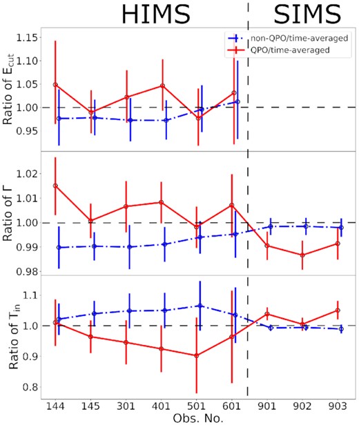
The spectral fitting parameters of nine observations. The model used is const*tbabs*(diskbb + cutoffpl), with NH fixed to |$3.8\times 10^{22} \rm \ cm^{-2}$|. The vertical axes are the ratio of the QPO/non-QPO fitting parameters to the corresponding time-averaged values. From top to bottom, the cutoff energy |$E_{\rm cut}^{\rm r}$|, photon index Γr, and inner disc temperature |$T_{\rm in}^{\rm r}$| are presented. The solid red lines represent the QPO regime, while the blue dash–dotted lines show the non-QPO regime. The non-QPO points are shifted a bit to the right to clearly show the ranges of error bars.
In order to understand the flux evolution of the spectral components, we estimated the flux of each model component by using cflux in xspec. We separately fitted LE (2–10 keV), ME (10–27 keV) and HE (27–100 keV) spectra for each component, and added them together. Table 3 presents the summed flux of 2–100 keV, and Fig. 7 shows the ratio of the QPO/non-QPO flux to the time-averaged flux. Both QPO and non-QPO unabsorbed fluxes |$F_{\rm unabsorb}^{\rm r}$| show a similar trend, except that the flux of the QPO regime is a little higher than the non-QPO flux, although some values have large errors. The power-law flux |$F_{\rm cpl}^{\rm r}$| exhibits an approximate trend to |$F_{\rm unabsorb}^{\rm r}$|, except in the SIMS, where the overlap between QPO and non-QPO regimes is more obvious. As for the disc flux |$F_{\rm disc}^{\rm r}$|, it is relatively steady throughout the nine observations in the non-QPO regime, but it variesin the QPO regime. The |$F_{\rm disc}^{\rm r}$| of QPO spectra is lower than that of non-QPO spectra in the HIMS, but has a sudden increase from the HIMS to the SIMS (the flux Fdisc also increases by about one order of magnitude from Obs 601 to 901, as seen in Table 3), and becomes approximately equal to or higher than the non-QPO |$F_{\rm disc}^{\rm r}$| when the source transits to the SIMS.

The summed flux of 2–100 keV with error bars. The vertical axes are the ratio of the QPO/non-QPO flux to the corresponding time-averaged flux. From top to bottom, the total flux |$F_{\rm unabsorb}^{\rm r}$|, cutoff power-law flux |$F_{\rm cpl}^{\rm r}$|, and disc flux |$F_{\rm disc}^{\rm r}$| are shown. The solid red lines represent the QPO regime, while the blue dash–dotted lines represent the non-QPO regime. The non-QPO points are shifted a bit to the right to clearly show the ranges of error bars.
The 2–100 keV summed flux values of the diskbb component, the cutoffpl component, and the total unabsorbed component.
| Obs | Fdisc(10−9) | Fcpl(10−9) | Funabsorb(10−9) |
|---|---|---|---|
| (erg/cm2/s) | (erg/cm2/s) | (erg/cm2/s) | |
| Time-averaged | |||
| 144 | |$4.95 _{- 0.18 }^{+ 0.23 }$| | |$97.47 _{- 1.34 }^{+ 1.58 }$| | |$102.81 _{- 1.29 }^{+ 1.38 }$| |
| 145 | |$4.90 _{- 0.20 }^{+ 0.23 }$| | |$98.77 _{- 1.03 }^{+ 1.36 }$| | |$104.03 _{- 1.16 }^{+ 1.03 }$| |
| 301 | |$6.21 _{- 0.37 }^{+ 0.38 }$| | |$113.68 _{- 1.59 }^{+ 1.69 }$| | |$119.99 _{- 1.39 }^{+ 1.72 }$| |
| 401 | |$5.68 _{- 0.37 }^{+ 0.38 }$| | |$120.50 _{- 1.39 }^{+ 1.69 }$| | |$126.51 _{- 1.59 }^{+ 1.58 }$| |
| 501 | |$4.39 _{- 0.27 }^{+ 0.28 }$| | |$133.78 _{- 1.00 }^{+ 1.76 }$| | |$139.11 _{- 1.55 }^{+ 1.75 }$| |
| 601 | |$5.00 _{- 0.25 }^{+ 0.57 }$| | |$138.09 _{- 2.07 }^{+ 2.41 }$| | |$143.60 _{- 1.92 }^{+ 2.25 }$| |
| 901 | |$41.50 _{- 0.61 }^{+ 0.61 }$| | |$135.75 _{- 3.13 }^{+ 3.11 }$| | |$177.64 _{- 2.29 }^{+ 2.43 }$| |
| 902 | |$43.09 _{- 0.60 }^{+ 0.59 }$| | |$134.58 _{- 2.84 }^{+ 2.96 }$| | |$177.70 _{- 2.20 }^{+ 2.43 }$| |
| 903 | |$33.39 _{- 0.73 }^{+ 1.08 }$| | |$142.94 _{- 3.95 }^{+ 3.95 }$| | |$177.91 _{- 3.36 }^{+ 3.39 }$| |
| Non-QPO | |||
| 144 | |$5.32 _{- 0.15 }^{+ 0.19 }$| | |$96.96 _{- 1.51 }^{+ 1.70 }$| | |$102.61 _{- 1.45 }^{+ 1.50 }$| |
| 145 | |$5.36 _{- 0.23 }^{+ 0.26 }$| | |$97.99 _{- 1.14 }^{+ 1.23 }$| | |$103.73 _{- 1.09 }^{+ 1.13 }$| |
| 301 | |$6.42 _{- 0.43 }^{+ 0.44 }$| | |$112.31 _{- 1.69 }^{+ 1.74 }$| | |$118.99 _{- 1.65 }^{+ 1.45 }$| |
| 401 | |$6.12 _{- 0.38 }^{+ 0.43 }$| | |$119.20 _{- 1.54 }^{+ 1.70 }$| | |$125.69 _{- 1.36 }^{+ 1.63 }$| |
| 501 | |$4.96 _{- 0.31 }^{+ 0.30 }$| | |$132.86 _{- 1.78 }^{+ 1.78 }$| | |$138.16 _{- 1.63 }^{+ 1.60 }$| |
| 601 | |$5.53 _{- 0.40 }^{+ 0.37 }$| | |$137.36 _{- 2.21 }^{+ 2.57 }$| | |$143.22 _{- 2.03 }^{+ 2.19 }$| |
| 901 | |$41.18 _{- 0.60 }^{+ 0.61 }$| | |$136.11 _{- 3.12 }^{+ 3.54 }$| | |$177.63 _{- 2.59 }^{+ 2.72 }$| |
| 902 | |$43.01 _{- 0.63 }^{+ 0.59 }$| | |$134.68 _{- 2.85 }^{+ 3.67 }$| | |$177.67 _{- 2.06 }^{+ 2.70 }$| |
| 903 | |$33.21 _{- 0.66 }^{+ 0.85 }$| | |$143.30 _{- 4.25 }^{+ 4.07 }$| | |$177.94 _{- 3.49 }^{+ 3.53 }$| |
| QPO | |||
| 144 | |$4.81 _{- 0.53 }^{+ 0.64 }$| | |$100.97 _{- 2.20 }^{+ 2.47 }$| | |$106.09 _{- 2.03 }^{+ 2.25 }$| |
| 145 | |$4.74 _{- 0.36 }^{+ 0.38 }$| | |$103.92 _{- 1.37 }^{+ 1.64 }$| | |$108.96 _{- 1.39 }^{+ 1.41 }$| |
| 301 | |$6.23 _{- 0.59 }^{+ 0.81 }$| | |$118.22 _{- 2.51 }^{+ 2.17 }$| | |$124.39 _{- 2.27 }^{+ 2.26 }$| |
| 401 | |$5.33 _{- 0.74 }^{+ 0.55 }$| | |$126.14 _{- 2.06 }^{+ 2.37 }$| | |$131.59 _{- 1.95 }^{+ 2.09 }$| |
| 501 | |$3.52 _{- 0.44 }^{+ 0.45 }$| | |$142.72 _{- 2.43 }^{+ 2.43 }$| | |$146.48 _{- 2.34 }^{+ 2.21 }$| |
| 601 | |$4.81 _{- 1.18 }^{+ 1.28 }$| | |$143.34 _{- 3.95 }^{+ 4.31 }$| | |$148.30 _{- 3.60 }^{+ 3.59 }$| |
| 901 | |$44.63 _{- 2.80 }^{+ 4.10 }$| | |$139.31 _{- 8.26 }^{+ 8.06 }$| | |$185.20 _{- 4.50 }^{+ 4.57 }$| |
| 902 | |$42.75 _{- 3.44 }^{+ 2.22 }$| | |$143.29 _{- 8.76 }^{+ 9.05 }$| | |$185.17 _{- 6.15 }^{+ 6.35 }$| |
| 903 | |$36.91 _{- 4.00 }^{+ 4.18 }$| | |$148.24 _{- 10.84 }^{+ 10.79 }$| | |$185.70 _{- 6.37 }^{+ 6.61 }$| |
The ratio of Fdisc to Funabsorb is plotted in Fig. 8 to show the evolution of the disc flux. Both QPO and non-QPO regimes show a sudden increase during the evolution from the HIMS to the SIMS. For the QPO regime, this ratio is lower in the HIMS compared with the non-QPO regime, but increases faster between Obs 601 and 901, and becomes similar to the ratio of the non-QPO regime in the SIMS.
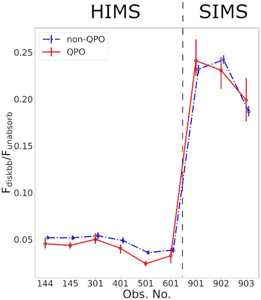
The proportion of the disc flux component defined by the ratio of Fdisc to Funabsorb. The solid red line is the QPO disc proportion, while the blue dash–dotted line is the non-QPO regime. The non-QPO points are shifted a bit to the right to clearly show the ranges of error bars.
Moreover, we plot Γ and Fdisc/Fcpl in Fig. 9 for Obs 106–918, where 106–108 and 906–918 are time-averaged data because they have no detected QPO signals, and 144–903 include the QPO and non-QPO separated data. QPO data and non-QPO data show diverse relationships in different states. During the HIMS (see the bottom right-hand panel of Fig. 9), a Spearman rank correlation test shows that the Spearman rank correlation r is –0.918 and the corresponding p-value is p = 0.009 for the QPO regime, and r = −0.940 with p = 0.005 for the non-QPO regime, indicating that the photon index has a negative relationship to the ratio of Fdisc/Fcpl. In addition, the QPO data have smaller Fdisc/Fcpl and slightly softer spectra compared with the non-QPO data. However, a different relationship appears in the case of the SIMS (see the bottom left-hand panel of Fig. 9), with r = 0.863 and p = 0.33, r = 0.970 and p = 0.15 for the QPO and non-QPO regimes, respectively, and the QPO spectra are harder and the disc components are becoming similar to the non-QPO data. Because there are only three data points in the SIMS, this marginal relationship between Γ and the flux ratio needs more observations to confirm it.

Photon index versus the ratio of the disc flux to the cutoff power-law flux (top panel). Both QPO and non-QPO points are presented for Obs 144–601 (red pentagons and blue inverted triangles, respectively) and Obs 901–903 (pink hexagons and green left-facing triangles, respectively). The time-averaged results of Obs 106–108 (orange circles) and 906–918 (purple crosses) without a QPO signal detected are also plotted. The diagrams for Obs 144–601 in the HIMS and for Obs 901–903 in the SIMS are also zoomed in on, for the better presentation of the QPO and non-QPO cases (bottom panel).
5 DISCUSSIONS AND CONCLUSIONS
In this work, we have applied the wavelet method to QPO analysis in X-ray binaries, and the time–frequency evolution of type-C QPOs in MAXI J1535–571 has been studied. The type-C QPOs show transient signals even on short time-scales (down to several seconds). With the wavelet method, we can separate the QPO and non-QPO events and derive the spectra for the QPO and non-QPO regimes, respectively. The wavelet results revealed the transitions between the QPO and non-QPO signals throughout the whole observations from the HIMS to the SIMS. The different spectral properties between QPO and non-QPO regimes may help in probing the origin of QPOs near a BH.
Xu et al. (2019) reported the sudden appearance of a type-C QPO, along with its flux decreasing by |$\sim45 {{\%}}$| in Swift J1658.2–4242. After comparing accumulated spectra before and after the flux change, they found that the emission of both the disc and the corona component decreased, with the disc temperature decreasing by |$\sim15 {{\%}}$|, but the inner disc radius and the coronal properties remained almost invariable. In the analysis of MAXI J1535–571 when QPOs are present, the diskbb norm parameter also shows no notable discrepancy in the SIMS, indicating that the inner edge of the accretion disc is stable (see Table 2). The disc temperature Tin of the QPO regime during the HIMS may systematically decrease (|$\sim10 {{\%}}$| on average, although large error bars exist, see Table 2) compared with the non-QPO regime, but there may also be a possibility that the non-QPO time intervals in the wavelet analysis contain some possible QPO time intervals with very low statistics for the QPO signal (e.g. below the |$95 {{\%}}$| confidence level), then Tin would not change significantly for the two regimes defined here. Moreover, instead of remaining unchanged as in Swift J1658.2–4242, the coronal property Γr in our source shows a relatively more pronounced variation as compared with |$T_{\rm in}^{\rm r}$| (see Fig. 6). Our total flux values also do not show the same trend as in the source Swift J1658.2–4242. On the contrary, the total flux in the QPO regimes is higher, as shown in Fig. 7. The sudden QPO appearance in Swift J1658.2–4242 may not have a similar origin to the fast evolution of the QPO phenomenon in MAXI J1535–571.
Zhang et al. (2021) analysed series of fast appearances and disappearances of type-B QPOs in the SIMS in MAXI J1348–630. They found that the spectral difference between the QPO and non-QPO regimes became significant above 2 keV, although a subtle difference existed below 2 keV (see their fig. 6). As a comparison, our 2–100 keV spectra in the SIMS (e.g. the bottom panel of Fig. 5) show a similar discrepancy. A difference between the QPO and non-QPO spectra also gradually became apparent, and the higher the energy, the greater the difference. However during the HIMS, the spectral difference of our data still existed in LE, but no obvious discrepancy can be noted in ME and HE (see the top panel of Fig. 5). Because the energy range of Zhang et al. (2021) is only up to 10 keV, we are unable to assert whether the part above 10 keV is similar to our SIMS spectra, or is consistent with our HIMS spectra. For the flux comparison, their disc and Comptonized components varied with the same behaviour as in our HIMS regime. Although type-B and type-C QPOs would have different physical origins, the transition between QPO and non-QPO regimes may have similar physics.
The spectral results on QPO and non-QPO regimes in this wavelet work combined with the QPO type work suggest that the differences between the HIMS and SIMS may be due to the sudden appearance of type-B QPOs in MAXI J1535–571. Type-C QPOs were studied in both the HIMS and the SIMS of MAXI J1535–571, and there are differences between QPO and non-QPO spectral behaviours from the HIMS to the SIMS. Insight-HXMT also found a strong type-B QPO signal just in the first ∼800 s of the dynamical PDS in Obs 701 (Huang et al. 2018), which just occurred around the dates between the HIMS and SIMS in our analysis. Sriram et al. (2021) reported a type-C to type-B transformation event in the source H1743–322, and the two-component hot flow model fitting suggested that the fundamental QPO and the harmonic were excited by an inner hot flow/jet and the outer part of a hot Compton component, respectively. They speculated that during the transition from type C to type B, the outer hot flow was ejected away, and only the inner part was left. This conjecture may explain our results on the spectral variation from the HIMS to the SIMS. There seems to be a visible increase in both the disc temperature and the flux during the evolution from the HIMS to the SIMS in our data (see Tables 2 and 3). If somehow the outer flow ejection occurred and covered part of the disc, then the departure of the outer part would cause a reduction of the proportion of the disc photons being Comptonized by the hot flow, leading to an increase of both the disc flux and the temperature.
It was thought that the observed QPOs might originate from the Lense–Thirring precession of the inner hot flow (Ingram et al. 2009; You et al. 2018, 2020). In this scenario, the ratio of the disc luminosity intercepted by the inner hot flow to the total disc-emitted luminosity reaches a maximum when the inner hot flow aligns with the disc. Those intercepted photons will be inverse-Compton-scattered in the precessing inner flow and illuminate the outer disc. Therefore, given the total disc-emitted luminosity, we would expect more Comptonized disc photons to illuminate and heat up the disc, when the flow aligns with the outer disc (see the upper panel of fig. 3 in You et al. 2018, and also Zycki, Done & Ingram 2016; Ingram & Motta 2019), which would lead to the increase of the disc temperature. Therefore, for the non-QPO time intervals during the HIMS when the precession is highly suppressed, the inner hot flow aligns with the disc, which would make the disc hotter. Such a scenario of the precession could also explain the harder non-QPO spectra in the HIMS. For the time intervals with non-QPOs, namely the inner hot flow being aligning with the outer disc, the disc luminosity is highly intercepted by the inner hot flow. This will lead to an increase of the Comptonization flux from the hot flow and a decrease of the disc flux. However, the hotter disc will create more radiation, which causes the total disc flux to increase or remain almost unchanged. The increased Comptonization flux may then be affected by the geometric change of the corona, or by a partial ejection of the Comptonized region as described in Sriram et al. (2021) and Zhang et al. (2021), resulting in a decrease in the line-of-sight flux, i.e. Fcpl.
In summary, we have studied the light curves of MAXI J1535–571 using wavelet analysis with the Insight-HXMT data. Nine observations are detected with QPO signals, and their spectra are divided into QPO and non-QPO regimes based on wavelet results. The relationship between QPO spectra and non-QPO spectra changes with evolution, which means that their physical mechanisms may not be the same. In the HIMS, the QPO regime has a lower disc temperature, softer spectra and lower disc flux compared with the non-QPO regime. These relations are reversed in the SIMS. The Comptonization flux and total flux in QPO spectra, however, are always higher, regardless of HIMS or SIMS.
The reversed relationship between the HIMS and SIMS may be related to the transient appearance of type-B QPOs in MAXI J1535–571, based on the wavelet results. A type-C to type-B transition was also reported by Sriram et al. (2021), but to analyse the connection and process between the two intermediate states, a complete C-B-C process analysis is needed with more observational data. Even though we cannot draw very convincing conclusions on the origin of QPO and non-QPO spectral behaviours owing to insufficient data, our results still reveal that wavelet analysis utilized in QPO study is an effective and promising method, and can be attempted in future QPO research.
ACKNOWLEDGEMENTS
We are very grateful to the referee for the fruitful suggestions for improving this manuscript. This work is supported by the National Key Research and Development Program of China (grants nos 2021YFA0718500, 2021YFA0718503), the National Natural Science Foundation of China (12133007, U1838103, 11622326, U1838201, U1838202, 11903024, U1931203), and the Fundamental Research Funds for the Central Universities (no. 2042021kf0224). This work made use of data from the Insight-HXMT mission, a project funded by China National Space Administration (CNSA) and the Chinese Academy of Sciences (CAS).
DATA AVAILABILITY
Data that were used in this paper are from the Institute of High Energy Physics Chinese Academy of Sciences(IHEP-CAS) and are publicly available for download from the Insight-HXMT website. To process and fit the spectrum and obtain folded light curves, this research has made use of xronos and ftools provided by NASA.
REFERENCES
APPENDIX A: COMPARISON OF DYNAMICAL POWER SPECTRUM AND WAVELET ANALYSIS
To extract time–frequency information from a signal, two possible methods can be used: one is the windowed Fourier transform (WFT), and the other is the wavelet transform. WFT is often used in the research of QPO signals, and the dynamical PDS generated by this technique is very helpful for analysing the sudden occurrence and disappearance of QPOs. However, this method has its drawbacks. First of all, the WFT is inefficient, because the T/2δt frequencies must be analysed at each time-step, where T is the length of a sliding segment (Torrence & Compo 1998). Secondly, as indicated by Kaiser (2011), the dividing line between time and frequency is determined by the choice of T, and thus we cannot assert whether the selected window contains exactly a certain frequency component. As a consequence, several values of T must be tested, but it is still possible to miss the appropriate results, which means it is difficult to make new discoveries. Wavelet analysis, as the other method, can solve both of the above problems, because this method is scale-independent. Furthermore, the global wavelet spectrum provided by the wavelet method is time-averaged, so it is smooth, unbiased and consistent, rather than full of noise and false peaks like the Fourier spectrum.
In order for readers to make a comparison, we show an example of the dynamical PDS results in Fig. A12. The data utilized in this plot are exactly the same as in Fig. 2, with the time resolution fixed at 1 s. RMS normalization (Miyamoto et al. 1991) is applied on the power. Compared with the wavelet plot, the WFT technique shows similar peak positions and numbers, but the time–frequency resolution is much lower.
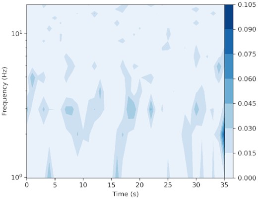
The dynamic PDS results derived with the same data as in Fig. 2. RMS normalization is applied on the power. A darker colour means a higher power.
To further confirm our wavelet result, we checked the light-curve data for QPO and non-QPO time ranges resolved by the 95 per cent confidence level of wavelet analysis as mentioned in Section 3.2, and Fourier transforms for the different light curves are performed for comparison. In Fig. A10, the QPO light curve and PDS are presented in the top panel, while the non-QPO light curve and corresponding PDS are in the bottom panel. The PDS and the error of power are produced from 2-s data intervals with rms normalization applied. The error of power relies on the number of averaging power spectra of segments of a light curve , and our time segments are too short, and thus the error bars are still large. Shorter data intervals will reduce errors, but the power spectrum becomes unreliable. Nevertheless, the QPO PDS still shows a clear background and a conspicuous peak with higher power at ∼2.5 Hz, but the non-QPO PDS is noisy, and the peak position is random and cannot be identified.
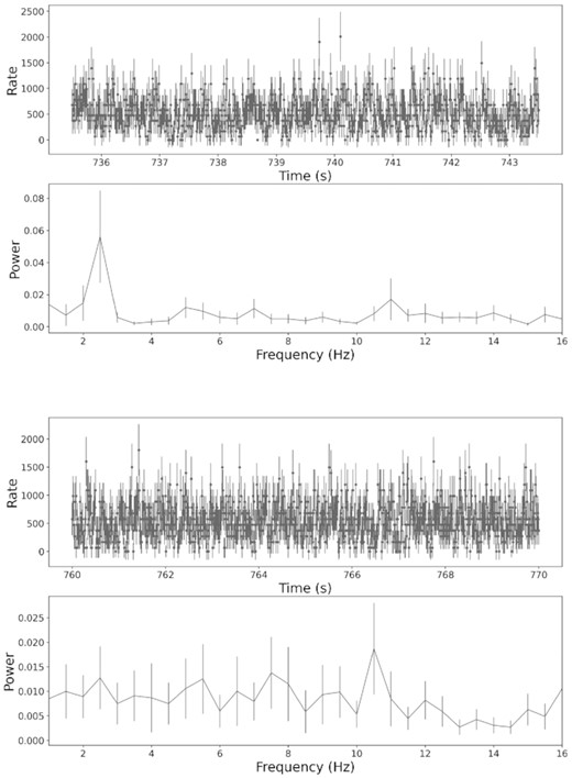
Examples of the light curves and corresponding power spectra for the time intervals of QPOs (top panel) and non-QPOs (bottom panel) identified by our wavelet method.
APPENDIX B: GTI COMPARISON OF THREE INSTRUMENTS
The wavelet analysis is better performed on continuous data, as large gaps in time series will reduce accuracy. After checking the GTI of our data, we believe that it is much safer to perform wavelet analysis on time series separated by GTIs for each observation. Fig. B11 presents the GTI distributions of Obs 501 and Obs 145. Normally, the HE and ME light curves are separated into ∼5 time series as in the top panel of Fig. B11, while the LE light curve contains 1 or 2 separated time series. The only different observation is Obs 145, which has a more scattered GTI distribution (see the bottom panel of Fig. B11).
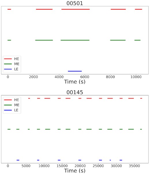
The GTIs of LE (blue), ME (green) and HE (red)for Obs 501 (top) and Obs 145 (bottom).
