


ABSTRACT
From a sample of 109 candidate ultrastrong Mg ii (USMg ii; having rest equivalent width of Mg ii, W2796 > 3.0 Å) systems at z = 0.4–0.6, we confirm 27 and identify host galaxies of 20 systems based on associated nebular line emission from our SALT observations or from Sloan Digital Sky Survey (SDSS) fiber spectra. The measured impact parameter, [O ii] luminosity, star formation rate, B-band luminosity, and stellar mass are in the ranges 7.3 ≤ D[kpc] ≤ 79, |$0.2\le L_{[\mathrm{ O}\,~\small {\rm II}]}[ 10^{41}~\mathrm{ erg} \mathrm{ s}^{-1}]\le 4.5$|, 2.59 ≤ SFR[M⊙yr−1] ≤ 33.51, |$0.15L_B^{*}\le L_B\le 1.63L_B^{*}$|, and 10.21 ≤ log[M*/ M ⊙] ≤ 11.62, respectively. The impact parameters found are larger than that predicted by the W2796 versus D relationship of the general population of Mg ii absorbers. At a given D, USMg ii host galaxies are more luminous and massive compared to typical Mg ii absorbers. However, the measured SFRs are slightly lower than that of main-sequence galaxies with same M⋆ at z ∼ 0.5. We report a correlation between |$L_{[\mathrm{ O}\,\small {\rm II}]}$| and W2796 for the full population of Mg ii absorbers, driven mainly by the host galaxies of weak Mg ii absorbers that tend to have low |$L_{[\mathrm{ O}\,\small {\rm II}]}$| and large impact parameters. We find at least ∼33 per cent of the USMg ii host galaxies (with a limiting magnitude of mr < 23.6) are isolated and the large W2796 in these cases may originate from gas flows (infall/outflow) in single haloes of massive but not starburst galaxies. We also find galaxy interactions could be responsible for large velocity widths in at least ∼17 per cent cases.
1 INTRODUCTION
Our current understanding of galaxy formation and evolution is based on the model known as the ‘cosmic baryon cycle’, according to which, galaxies evolve by means of a slowly varying equilibrium between inflows from the intergalactic medium (IGM), high velocity outflows from the galaxy and the in situ star formation taking place within the galaxy (Anglés-Alcázar et al. 2017; Péroux & Howk 2020). Biconical galactic scale outflows (with velocities of 100–1000 |$\mathrm{ km}\, \mathrm{ s}^{-1}$|), probed by neutral or singly ionized species like Na i, Mg ii, and Fe ii in absorption, are ubiquitous in high redshift (i.e. 0.5 ≤ z ≤ 1.5) galaxies (e.g. Tremonti, Moustakas & Diamond-Stanic 2007; Chen et al. 2010a; Martin et al. 2012; Bordoloi et al. 2014; Rubin et al. 2014). The probability to detect a wind is found to depend weakly on the intrinsic properties of the galaxies but strongly on the galaxy orientation. Notwithstanding this, the importance of star formation rate (SFR) and stellar mass (M*) of the host galaxy is reflected by the correlations observed between the maximum wind velocity (vmax) and M*, and between the equivalent width of the flow and SFR. While the presence of a wind is well established in these galaxies, its location (important for deriving wind parameters) with respect to the stellar disc cannot be constrained accurately.
On the other hand, quasar absorption lines in principle allow us to probe the spatial distribution and kinematics of the gas in foreground galaxies at very small impact parameters (D), thereby allowing us to probe the nature of gas flows in these galaxies. Presence of cool circumgalactic medium (CGM) around galaxies out to projected distances of ∼200 kpc (for e.g. Bergeron & Boissé 1991; Steidel 1995; Chen et al. 2010a; Nielsen, Churchill & Kacprzak 2013a; Rubin et al. 2018) is well established and an anticorrelation between the rest equivalent width of Mg ii λ2796 absorption (i.e. W2796) and the impact parameter has been derived using spectra of distant quasars. While early models reproduced this correlation using photoionized haloes around galaxies (see e.g. Petitjean, Bergeron & Puget 1992; Srianand & Khare 1994), it was apparent that continuous gas flow is needed to sustain the observed covering fraction of gas over a long period.
This observed anticorrelation between W2796 and D allows us to select quasar and foreground galaxy pairs with small impact parameters using absorption systems with large |$\rm {\mathit{ \mathit{ W}}_{2796}}$| (see Bouché et al. 2007, 2012). The Mg ii absorption systems with W2796 > 3 Å are known as UltraStrong Mg ii absorbers (referred hereafter as USMg ii; Nestor et al. 2011a). They constitute only 0.8 per cent of the Mg ii absorber population having W2796 > 0.02 Å. Observationally such large equivalent widths are seen in a very high fraction (i.e 30–50 per cent) of (i) outflows detected in z ∼ 0.5 galaxies (Rubin et al. 2014); (ii) Milky Way sightlines that probe disc + halo gas (after applying a factor 2 correction to match with QSO absorbers, Savage et al. 2000); (iii) Galaxy On Top Of Quasars (GOTOQs; Noterdaeme et al. 2010b; Straka et al. 2015; Joshi et al. 2017, 2018) and (iv) high-z C i absorbers (Ledoux et al. 2015; Zou et al. 2018). From fig. 2 of Rao et al. (2017) it is also evident that more than 50 per cent of USMg ii absorbers are damped Lyman α systems (DLAs; neutral hydrogen column density, N(H i) ≥ 2 × 1020 cm−2).
It is well known that the measured W2796 using low dispersion spectra are related to the number of absorbing clouds and velocity dispersion between them, and not directly related to the column density (Petitjean & Bergeron 1990). For a fully saturated Mg ii line, W2796 ≥ 3 Å; would correspond to a minimum velocity width of 320 |$\rm {km\, s^{-1}}$|. Gas having such velocity spread usually have large metallicities (Ledoux et al. 2006). Large velocity spread could originate from, (i) galactic-scale outflows (Bouché et al. 2006; Weiner et al. 2009; Rubin et al. 2012), (ii) filamentary accretion on to galaxies (Steidel et al. 2002; Chen et al. 2010a), (iii) dynamical mergers (Richter 2012) and intragroup gas (Rubin et al. 2010; Gauthier 2013). In such cases, measured metallicities and galaxy orientations with respect to the quasar sightlines are used to distinguish between the different possibilities (Bordoloi et al. 2011; Péroux et al. 2013; Kacprzak et al. 2014; Zabl et al. 2019; Péroux et al. 2020; Zabl et al. 2021).
It is possible that absorption line-based selection of galaxies (unbiased by the galaxy luminosity) may pick a population that is different from that observed through galaxy surveys that rely on optical colours and emission line strengths. Large W2796 systems, in particular the USMg ii systems have been associated with host-galaxies that are going through a rapid star formation episode or have been through a phase of rapid star formation in the recent past, i.e. they are either starburst or post-starburst galaxies (Nestor et al. 2011a). By studying the average photometric properties of more than 2800 Mg ii systems, Zibetti et al. (2007) suggested that the stronger Mg ii systems (with W2796 ≥ 1 Å) are associated with actively star-forming galaxies. Based on the [O ii] emission associated with Mg ii-selected systems, Noterdaeme, Srianand & Mohan (2010a) found a strong correlation between W2796 and [O ii] luminosity. In a similar work, Ménard et al. (2011) interpreted this as a correlation between W2796 and SFR, but this interpretation was later shown to be vulnerable to fiber losses effects (López & Chen 2012; Joshi et al. 2017).
Discussions presented above suggests that USMg ii absorbers are ideal targets for studying the gas flows at low impact parameters to star-forming galaxies and/or interacting groups of galaxies. Studying such systems can provide important insights into the baryonic cycle that governs the galaxy evolution. Motivated by this, we embarked on a detailed study of USMg ii systems at z ∼ 0.5 with the aim to (i) identify their host galaxies and characterize the galaxy environment around these absorbers, (ii) investigate whether we preferentially select a particular galaxy population using the USMg ii selection, (iii) study the connection between the galaxy properties and that of the absorption features, and (iv) identify potential quasar–galaxy pairs where galactic outflow can be studied through down-the-barrel absorption towards the galaxy, and absorption along the quasar line of sight simultaneously. This paper is organized as follows. In Section 2, we discuss the sample. The observational setup, data reduction, and calibrations are described in Section 3. The identification of the USMg ii host galaxies and the method of inferring their physical properties based on the available spectrophotometric data are discussed in Section 4. In Section 5, we present the results of our analysis and the nature of the USMg ii host galaxies based on the inferred galaxy properties. As we go along, to investigate whether the USMg ii host galaxies are drawn from a specific galaxy population or not, we compare their properties against various low-z Mg ii and DLA absorber samples available in the literature. Wherever possible, we also compare the properties of our sample with those of high-z C i absorbers. In Section 6, we provide an overall discussion on the USMg ii systems. Our conclusions are summarized in Section 7. Throughout this paper we assume a flat ΛCDM cosmology with |$H_0 = 70\, \rm {km\, s^{-1}\, Mpc^{-1}}$| and Ωm, 0 = 0.3.
2 OUR SAMPLE OF USMG ii SYSTEMS AT Z ∼ 0.5
We compiled a sample of USMg ii systems that are accessible to the South African Large Telescope (SALT; Buckley et al. 2005) (i.e. declination, δ ≤ +10°), using the Sloan Digital Sky Survey (SDSS; York et al. 2000) Mg ii/Fe ii absorber catalogue of Zhu & Ménard (2013) in the redshift range 0.4 ≤ zabs ≤0.6. The lower limit in zabs was chosen so that the SDSS spectra could cover the Fe ii λ2600 absorption line, while the upper limit on zabs is set to be able to cover the [O ii] λλ3727, 3729 doublet, H β and [O iii] λλ4960, 5008 nebular emission lines associated with the USMg ii absorption, in the wavelength range over which the Robert-Stobie Spectrograph (RSS) attached to SALT has good sensitivity. Application of these criteria has resulted in a total of 109 USMg ii systems along the line of sight towards 106 different background quasars. A careful visual inspection of the SDSS spectrum of each of these quasars has led to the removal of 34 systems from our sample owing to the false identification of Mg ii doublets. In 48 cases, C iv or Si iv broad absorption lines (BAL) are misidentified as Mg ii. After removing these we are left with a sample of 27 USMg ii systems.
Details of all the 109 USMg ii systems retrieved from the SDSS Mg ii / Fe ii absorber catalogue of Zhu & Ménard (2013) are provided in the table B1 in the Appendix, where we have explicitly mentioned the reason for rejecting or accepting a USMg ii system in our sample along with information such as the quasar and absorption redshifts. Among these 27 systems, the galaxy association for 3 USMg ii systems have already been studied in the literature in some detail. One is the mutiband photometric study of the environment of the USMg ii system J0240−0812 (Nestor et al. 2007), and another is the spectrophotometric study of the USMg ii system J2207−0901 (Gauthier 2013). In addition, using the X-shooter spectrograph at the Very Large Telescope, Rahmani et al. (2016) have studied the galaxy associated with the z = 0.5896 USMg ii absorber, which is a known DLA. The [O ii] nebular emission from another three of our USMg ii systems (i.e. zabs = 0.5928 towards J0930+0018, zabs = 0.5561 towards J1025−0046 and zabs = 0.5519 towards J1216+0350) were detected in the SDSS spectrum and these systems are part of the GOTOQ sample of Joshi et al. (2017).
In order to reconfirm that all the selected Mg ii systems are bonafide USMg ii systems, we measured the rest equivalent widths of Mg ii λλ2796, 2803 absorption lines by Gaussian fitting after approximating the observed continuum spectrum around these absorption lines with smooth polynomials. Our Gaussian fits to absorption lines are shown in figs A1 and A2 in the Appendix. During the fit, we kept the redshift and the velocity width same for both the lines of the Mg ii doublet. For the USMg ii systems in the spectrum of J0334−0711, J0856+0740, J2045−0704 and, J1114−0023, even at SDSS resolution, the Mg ii|$\lambda \, 2796$| absorption line itself splits into two Gaussian profiles. For these systems, we fit the Mg ii λλ2796, 2803 absorption profile with a pair of Gaussian doublets. For each pair, like before, we imposed the redshift and the velocity width for the individual Gaussian to be same. While the total equivalent width is greater than 3 Å, except for J1114−0023, individual components in these systems are not USMg ii absorbers. For these systems, we quote the mean redshift of the pair of Gaussian doublets as the absorption redshift. Our analysis confirmed that all the 27 systems selected are indeed USMg ii absorbers. Similarly, we also measured the rest equivalent width of the other associated absorption lines like Fe ii|$\lambda \, 2600$| and Mg i|$\lambda \, 2853$| by fitting a single Gaussian (also shown in Fig. A1). The complete sample along with their absorption properties are presented in Table 1. In this table, the quasar name, zqso, and zabs are summarized in columns 2, 3, and 4, respectively. The next four columns provide rest equivalent widths of Mg ii λ2796, Mg ii λ2803, Fe ii λ2600, and Mg i λ2853, respectively. For the cases with detection significance level less than 3σ, we provide the 3σ upper limits. For these cases, the 1σ limit is computed from the total uncertainty across the FWHM of the Mg ii absorption line profile around the expected location of the absorption line of our interest.
Details of our USMg ii sample. Columns 2, 3, and 4 provide the quasar name, its redshift, and the USMg ii absorption redshift, respectively. The next four columns (i.e. 5–8) provide the rest equivalent width of Mg ii|$\lambda \, 2796$|, Mg ii|$\lambda \, 2803$|, Fe ii|$\lambda \, 2600$|, and Mg i|$\lambda \, 2853$| absorption, respectively, where ‘−’ signifies the absorption is outside of the wavelength coverage of the observed spectrum. In the case of non-detections, we provide 3σ upper limits. Last column provides the measured E(B−V) derived using the SMC extinction curve.
| No. | Quasar | zqso | zabs | |$W_{2796}\, (\mathring{\rm A})$| | |$W_{2803}\, (\mathring{\rm A})$| | |$W_{2600}\, (\mathring{\rm A})$| | |$W_{2853}\, (\mathring{\rm A})$| | |$\rm {E(B-V)\, (SMC)}$| |
|---|---|---|---|---|---|---|---|---|
| (1) | (2) | (3) | (4) | (5) | (6) | (7) | (8) | (9) |
| Targets with SALT spectrum | ||||||||
| 1 | J000413.73−082625.4 | 2.247 | 0.5544 | 3.07 ± 0.16 | 3.05 ± 0.15 | 2.05 ± 0.15 | 0.82 ± 0.15 | 0.015 ± 0.002 |
| 2 | J015635.18+034308.1 | 1.371 | 0.5581 | 4.20 ± 0.30 | 3.76 ± 0.26 | 3.30 ± 0.40 | 1.56 ± 0.26 | 0.199 ± 0.001 |
| 3 | J021820.10−083259.4a | 1.219 | 0.5896 | 3.07 ± 0.11 | 2.81 ± 0.10 | 2.15 ± 0.14 | 1.43 ± 0.14 | 0.022 ± 0.001 |
| 4 | J024008.21−081223.4b | 2.230 | 0.5311 | 3.88 ± 0.17 | 3.56 ± 0.16 | 2.01 ± 0.15 | ≤0.89 | 0.015 ± 0.005 |
| 5 | J033438.28−071149.0 | 0.634 | 0.5977 | 3.55 ± 0.23 | 3.13 ± 0.24 | 1.89 ± 0.22 | 0.34 ± 0.01 | −0.011 ± 0.001 |
| 6 | J085627.09+074031.7 | 1.890 | 0.5232 | 4.14 ± 0.47 | 3.19 ± 0.61 | 1.22 ± 0.20 | 0.34 ± 0.05 | 0.197 ± 0.001 |
| 7 | J092222.58+040858.7 | 0.713 | 0.4549 | 3.63 ± 0.21 | 3.11 ± 0.18 | – | 0.72 ± 0.12 | 0.049 ± 0.003 |
| 8 | J111400.00−002342.6 | 0.952 | 0.5610 | 5.75 ± 1.36 | 4.62 ± 1.33 | 3.33 ± 0.95 | 2.40 ± 0.47 | 0.102 ± 0.004 |
| 9 | J121453.29+080457.7 | 1.430 | 0.4908 | 3.38 ± 0.21 | 2.97 ± 0.19 | 2.27 ± 0.12 | ≤0.63 | 0.089 ± 0.003 |
| 10 | J121628.03+035031.8d | 0.996 | 0.5519 | 3.51 ± 0.12 | 3.53 ± 0.12 | 2.89 ± 0.18 | 0.81 ± 0.12 | −0.063 ± 0.001 |
| 11 | J155003.71+031325.0 | 1.789 | 0.5694 | 3.11 ± 0.08 | 2.97 ± 0.08 | 1.82 ± 0.15 | 1.04 ± 0.16 | 0.141 ± 0.004 |
| 12 | J204501.32−070452.6 | 0.670 | 0.5649 | 3.77 ± 0.28 | 3.12 ± 0.32 | 2.37 ± 0.15 | 1.21 ± 0.38 | 0.059 ± 0.003 |
| 13 | J210851.53−074726.5 | 1.486 | 0.5187 | 3.43 ± 0.17 | 2.69 ± 0.14 | 2.24 ± 0.24 | 1.43 ± 0.25 | 0.088 ± 0.003 |
| 14 | J212143.98+003954.2 | 1.348 | 0.5509 | 3.44 ± 0.33 | 3.57 ± 0.34 | 2.85 ± 0.48 | 1.60 ± 0.24 | 0.132 ± 0.003 |
| 15 | J212727.20+082724.6 | 0.745 | 0.4392 | 4.26 ± 0.16 | 3.99 ± 0.15 | 3.75 ± 0.16 | 1.28 ± 0.13 | 0.042 ± 0.001 |
| 16 | J220330.04−002211.4 | 1.782 | 0.4381 | 4.49 ± 0.31 | 3.99 ± 0.27 | − | 0.82 ± 0.13 | 0.022 ± 0.002 |
| 17 | J220702.53−090127.7c | 1.296 | 0.5623 | 4.08 ± 0.18 | 3.66 ± 0.16 | 2.93 ± 0.32 | 1.39 ± 0.14 | 0.047 ± 0.002 |
| 18 | J230101.28−021200.0 | 0.619 | 0.5367 | 3.16 ± 0.07 | 3.07 ± 0.07 | 2.20 ± 0.12 | 0.65 ± 0.07 | 0.086 ± 0.001 |
| 19 | J232653.15+002142.9 | 2.190 | 0.5624 | 4.37 ± 0.46 | 5.22 ± 0.55 | 4.29 ± 0.76 | 2.00 ± 0.23 | 0.013 ± 0.007 |
| 20 | J233548.62−023734.3 | 1.234 | 0.5081 | 3.76 ± 0.10 | 3.57 ± 0.10 | 2.54 ± 0.11 | 1.15 ± 0.13 | 0.047 ± 0.002 |
| 21 | J233818.25−005610.5 | 0.894 | 0.4801 | 3.05 ± 0.12 | 2.74 ± 0.10 | 1.95 ± 0.31 | 0.51 ± 0.08 | −0.018 ± 0.003 |
| Targets without SALT spectrum | ||||||||
| 22 | J093020.60+001828.0d | 2.4300 | 0.5928 | 3.48 ± 0.25 | 3.58 ± 0.25 | 2.90 ± 0.22 | 1.75 ± 0.36 | −0.101 ± 0.004 |
| 23 | J101610.82+075209.1 | 2.187 | 0.5961 | 3.09 ± 0.38 | 3.62 ± 0.45 | 2.04 ± 0.20 | 1.31 ± 0.17 | 0.028 ± 0.006 |
| 24 | J102510.10−004644.9d | 2.212 | 0.5561 | 3.22 ± 0.11 | 2.80 ± 0.10 | 2.05 ± 0.08 | 0.97 ± 0.07 | 0.037 ± 0.001 |
| 25 | J103059.75−013237.7 | 2.155 | 0.5783 | 3.27 ± 0.10 | 3.20 ± 0.10 | 2.39 ± 0.11 | 0.49 ± 0.01 | −0.024 ± 0.001 |
| 26 | J110817.93+062833.0 | 1.202 | 0.5721 | 3.02 ± 0.16 | 2.89 ± 0.15 | 1.72 ± 0.33 | 0.49 ± 0.16 | 0.023 ± 0.004 |
| 27 | J114614.24−023716.1 | 2.207 | 0.5295 | 4.13 ± 0.22 | 3.22 ± 0.17 | ≤0.59 | ≤0.91 | −0.227 ± 0.004 |
| The non-USMg ii absorber in our lines of sight | ||||||||
| 28 | J111400.00−002342.6 | 0.952 | 0.7981 | 2.15 ± 0.18 | 1.88 ± 0.16 | 1.37 ± 0.16 | 0.42 ± 0.09 | 0.084 ± 0.006 |
Host galaxy of this USMg ii system was studied by Rahmani et al. (2016) using both spectroscopy and multiband photometry.
The environment of this system was explored in Nestor et al. (2007) using multiband photometry.
A group of 4 galaxies associated with this USMg ii was studied by Gauthier (2013) using both spectroscopy and multiband photometry.
These systems are part of the GOTOQ sample of Joshi et al. (2017).
Next, we identified additional non-USMg ii absorber in the SDSS spectra of quasars in our sample. We find 11 Mg ii systems but none at 0.4 ≤ zabs ≤ 0.6. We then tried to identify if any of the targeted potential host galaxies corresponds to the non-USMg ii absorbers identified in the spectra of our sample. We found only one system at zabs = 0.7981 (|$\rm {\mathit{ W}_{2796} = 2.14\pm 0.18}$|Å) towards J1114−0023. We provide the details of this absorber in the last row of Table 1.
2.1 Line-of-sight reddening towards quasars
We calculate the reddening of the background quasar by the absorbing gas assuming the extinction curve of the gas to be similar to the extinction curves of the Small Magellanic Cloud (SMC), Large Magellanic Cloud (LMC), Large Magellanic Cloud Supershell (LMC2) and, our Milky Way (MW) Galaxy (Gordon et al. 2003). For the rest wavelength range considered here, the choice of different extinction curves are found to make no significant difference. We fitted all the quasar spectra in our sample with a standard quasar spectrum template (Selsing et al. 2016) redshifted exactly to the quasar redshift and applied the SMC extinction at the redshift of the USMg ii absorption, keeping the V-band extinction coefficient, AV, as the only free parameter, apart from a multiplicative scaling (as described in Srianand et al. 2008). The best fit V-band colour excess, E(B−V), for each system is listed in the last column of Table 1.
In Fig. 1, the distribution of E(B−V) is shown in the left panel. For 6 USMg ii systems, we find that the colour excess, E(B−V) is negative. The system J1146−0237 has an extremely negative E(B−V) of −0.227, which is related to the fact that the quasar has weak emission lines and its spectrum does not exactly follow the standard quasar template. We used the remaining cases with negative values of E(B−V) to compute the expected scatter from the spectral energy distribution (SED) fitting procedure. The deep blue Gaussian shown in Fig. 1 corresponds to the distribution of E(B−V) (with a σ = 0.050) that is expected to arise from our template matching procedure. The vertical dashed green line corresponds to the 3σ limit of our E(B−V) measurements. We find only two USMg ii systems present in our sample to have E(B−V) larger than this value. The highest E(B−V) of ∼0.2 is measured for J0156+0343. As this is a C iv BAL quasar, it is not clear how much of the reddening is due to the USMg ii absorber.

Left-hand panel: The histogram of the V band colour excess, E(B−V), for the USMg ii systems in our sample. The deep blue Gaussian (μ = 0, σ = 0.050) corresponds to the distribution of E(B−V) that is expected to arise out of the template matching procedure. We inferred this from the distribution of negative E(B−V) values in our sample (see text for more details). The vertical dashed green line corresponds to the 3σ above the mean of the distribution. The solid vertical black line corresponds to the expected colour excess for the |$\rm {\mathit{ W}_{2796} = 3}$|Å based on the relation obtained by Budzynski & Hewett (2011) with the grey region showing the 1σ uncertainty range. The vertical red line corresponds to the median colour excess for our USMg ii sample. Right-hand panel: Comparison of the distribution of colour excess, E(B−V), between the USMg ii absorbers (blue histogram) and C i absorbers (orange histogram) taken from Ledoux et al. (2015). The solid blue and red lines correspond to the cumulative distribution of E(B−V) for the USMg ii and C i absorbers, respectively.
Using a sample of about 8300 strong Mg ii absorption systems identified in the SDSS spectroscopic survey (DR6), Budzynski & Hewett (2011) have shown that |$\rm {\mathit{ W}_{2796}}$| strongly correlates with reddening of the background quasar spectra (see also, York et al. 2006; Ménard et al. 2008) with E(B−V) = [(8.0 ± 3.0) × 10−4] × (W2796)(3.48 ± 0.3). The solid vertical black line in the left-hand panel of the Fig. 1 corresponds to the expected |$\rm {\mathit{ E}(\mathit{ B}-\mathit{ V})}$| for the |$\rm {\mathit{ W}_{2796}} = 3\mathring{\rm A}$| based on this relationship. The solid vertical red line corresponds to the median colour excess of our USMg ii sample. Higher E(B−V) seen in our sample is consistent with their results.
In the right-hand panel of Fig. 1, the blue and orange histograms correspond to the E(B−V) measurements for USMg ii and high-z C i- selected absorbers from Ledoux et al. (2015), respectively. The solid blue and red lines correspond to the cumulative distribution function for the USMg ii and C i absorbers, respectively. The median E(B−V) values for the USMg ii and C i absorbers are 0.037 and 0.042, respectively. A two sample Kolmogorov–Smirnov (KS) test between these two samples indicates that the probability of these two samples to arise from the same parent population is ∼80 per cent. This is not surprising given the fact that a good fraction (i.e. ∼47 per cent) of C i absorbers have W2796 > 3.0 Å; (see table 2 of Zou et al. 2018).
Log of observations for our USMg ii sample. Systems marked with * represent non-detection of any associated host galaxy, while systems marked with + represent cases where the host galaxy sits on top of the quasar along the line of sight (see text for more details). The last two columns correspond to the number of other candidate galaxies within 50 ≤D[kpc] ≤ 100 and D ≤ 50 kpc with mr ≤ 22.5 based on SDSS photometry.
| No. | Quasar | Date | Exposure (s) | Observation | PA (deg.) | Grating | Wavelength | Other candi- | Total candi- |
|---|---|---|---|---|---|---|---|---|---|
| Mode | Angle (deg) | range (Å) | date galaxies | date galaxies | |||||
| (50 ≤ D[kpc] ≤ 100) | (D ≤ 50 kpc) | ||||||||
| (1) | (2) | (3) | (4) | (5) | (6) | (7) | (8) | (9) | (10) |
| 1 | J000413.73−082625.4 | 2017-07-18 | 2400 | Long-slit | 80 | 17.75 | 5200–8200 | 0 | 1 |
| 2017-09-17 | 2400 | Long-slit | 80 | 17.75 | 5200–8200 | ||||
| 2 | J015635.18+034308.1 | 2015-11-07 | 2500 | Long-slit | 350 | 17.00 | 4900–7900 | 0 | 5 |
| 2015-11-13 | 2500 | Long-slit | 350 | 17.00 | 4900–7900 | ||||
| 3 | J021820.10−083259.4 | 2016-01-10 | 2500 | Long-slit | 80 | 18.125 | 5300–8300 | 0 | 1 |
| 4 | J024008.21−081223.4 | 2018-10-05 | 2500 | Long-slit | 80 | 17.75 | 5200–8200 | 0 | 1 |
| 5 | J033438.28−071149.0 | 2017-11-19 | 2300 | MOS | 44.8 | 17.75 | 5200–8200 | 0 | 1 |
| 2017-12-11 | 2300 | MOS | 44.8 | 17.75 | 5200–8200 | ||||
| 6 | J085627.09+074031.7 | 2018-02-09 | 2200 | Long-slit | 315 | 17.00 | 4900–7900 | 0 | 1 |
| 2018-02-10 | 2200 | Long-slit | 315 | 17.00 | 4900–7900 | ||||
| 7 | J092222.58+040858.7 | 2016-02-08 | 2400 | Long-slit | 0 | 16.625 | 4800–7800 | 0 | 1 |
| 2016-03-01 | 2400 | Long-slit | 0 | 16.625 | 4800–7800 | ||||
| 8 | J111400.00−002342.6 | 2021-04-15 | 2580 | Long-slit | 0 | 18.125 | 5300–8300 | 1 | 1 |
| 9 | J121453.29+080457.7 | 2016-04-09 | 2300 | Long-slit | 100 | 17.375 | 5050–8050 | 1 | 1 |
| 2016-03-01 | 2160 | Long-slit | 100 | 17.375 | 5050–8050 | ||||
| 10 | J121628.03+035031.8 + | 2016-02-05 | 2400 | Long-slit | 0 | 17.75 | 5200–8200 | 0 | 1 |
| 2016-02-06 | 2400 | Long-slit | 90 | 17.75 | 5200–8200 | ||||
| 11 | J155003.71+031325.0 | 2015-06-19 | 2500 | Long-slit | 96 | 16.625 | 4800–7800 | 0 | 1 |
| 2015-07-14 | 2500 | Long-slit | 96 | 18.125 | 5300–8300 | ||||
| 12 | J204501.32−070452.6 * | 2017-08-18 | 2500 | Long-slit | 77 | 18.125 | 5300–8300 | 0 | 1 |
| 13 | J210851.53−074726.5 + | 2017-06-03 | 2400 | Long-slit | 70 | 17.75 | 5200–5300 | 0 | 1 |
| 2017-06-18 | 2400 | Long-slit | 70 | 17.75 | 5200–5300 | ||||
| 14 | J212143.98+003954.2 | 2015-06-20 | 2340 | Long-slit | 90 | 16.625 | 4800–7800 | 0 | 1 |
| 2020-10-18 | 2200 | Long-slit | 240 | 18.125 | 5300–8300 | ||||
| 15 | J212727.20+082724.6 | 2015-06-18 | 2500 | Long-slit | 95 | 16.625 | 4800–7800 | 0 | 1 |
| 2016-06-20 | 1844 | Long-slit | 95 | 18.125 | 5300–8300 | ||||
| 16 | J220330.04−002211.4 | 2017-09-13 | 2500 | Long-slit | 45 | 17.00 | 4900–7900 | 0 | 1 |
| 17 | J220702.53−090127.7 | 2017-09-16 | 2400 | Long-slit | 77 | 18.125 | 5300–8300 | 1 | 1 |
| 18 | J230101.28−021200.0 * | 2017-10-11 | 2500 | Long-slit | 308 | 18.125 | 5300–8300 | 0 | 0 |
| 2017-10-17 | 2500 | Long-slit | 283 | 17.375 | 5050–8050 | ||||
| 19 | J232653.15+002142.9 | 2017-10-17 | 2500 | Long-slit | 5 | 18.125 | 5300–8300 | 0 | 1 |
| 20 | J233548.62−023734.3 | 2015-06-19 | 2271 | Long-slit | 100 | 16.625 | 4800–7800 | 0 | 1 |
| 2015-06-21 | 2500 | Long-slit | 100 | 18.125 | 5300–8300 | ||||
| 21 | J233818.25−005610.5 | 2018-08-21 | 2200 | MOS | 90 | 17.00 | 4900–7900 | 1 | 1 |
| 2018-09-11 | 2324 | MOS | 90 | 17.00 | 4900–7900 |
2.2 Detection of other metal lines
Out of the 27 USMg ii systems, six (along the line of sight of J0240−0812, J1016+0752, J1025−0046, J1030−0132, J1216+0350, and J2301−0212) exhibit associated Mn ii absorption having more than |$\rm {3\sigma }$| significance (see fig. A1 in the Appendix) with the rest equivalent width in the range, |$0.25\le \rm {\mathit{ W}_{2576}^{Mn\small {\rm II}}}(\mathring{\rm A})\le 1.32$|, while 10 systems (along the line of sight of J0218−0832, J0334−0711, J1025−0046, J1114−0023, J1214+0804, J1216+0350, J2121+0039, J2127+0827, J2203−0022 and J2301−0212) exhibit associated Ca ii absorption (see fig. A2 in the Appendix) with the rest equivalent width in the range (|$0.18\le \rm {\mathit{ W}_{3935}^{Ca\small {\rm II}}}(\mathring{\rm A})\le 1.08$|) in the SDSS spectra of the background quasars. In the case of non-detection, the |$\rm {3\sigma }$|, upper limits are typically in the range 0.5–0.9 Å. We do not find any significant correlation between |$\mathrm{\mathit{ W}^{CaII}_{3935}}$| and E(B−V). In addition, the distributions of measured E(B−V) of sightlines with and without Ca ii detected are not statistically different (KS test p-value = 0.23).
For the sake of comparison, in fig. D1 in the Appendix, we plot E(B−V) versus Ca ii equivalent width in our sample with those found in low-z DLAs (Wild & Hewett 2005), high-z C i sample (Zou et al. 2018) and our Galaxy (Murga et al. 2015). We do not detect associated Na i absorption (at >3σ level) for any of the USMg ii systems in our sample in the SDSS spectrum. The |$\rm {3\sigma }$| upper limit on the rest equivalent width lies between 0.5 and 0.9 Å. As our SALT spectra cover limited wavelength range we could not use them for the above discussed absorption line searches.
3 SALT OBSERVATIONS AND DATA REDUCTION
We first identified all galaxies seen within an impact parameter of 50 kpc from the quasar line of sight using the SDSS photometry (typically complete for mr ≤ 22.5) and having consistent photometric redshifts within 1σ. Note that based on the known anticorrelation between D and W2796, we expect the isolated host galaxies to lie within D ≤ 10 kpc. Even with the scatter in the relation the observed D values are <50 kpc in the available literature data (see discussions in Section 5.4). Thus we mainly focus on observing candidate galaxies within this impact parameter. We have completed observations for 21 absorbers out of 27 discussed in the previous section.
In Table 2, we provide the number of such galaxies (last column) in addition to our observational log. It is clear from this table that in only one case we have more than one host-galaxy candidate within 50 kpc. These are 5 galaxies in the case of zabs = 0.5581 towards J0156+0343 within 50 kpc. In 6 cases the potential galaxy image is merged with that of the quasar (see Fig. 2). Thus we have 26 host galaxy candidates and we obtained spectra of 23 of them (including from the literature as mentioned above). The SALT spectroscopic observations were carried out using the Robert Stobie Spectrograph (RSS; Burgh et al. 2003; Kobulnicky et al. 2003) either in the long-slit or the Multi Object Spectroscopy (MOS) mode from June, 2015 to April, 2021 (Program IDs: 2015-1-SCI-021, 2015-2-SCI-031, 2017-1-SCI-011, 2017-2-SCI-009 and 2018-1-SCI-019, 2020-2-SCI-019).
![The DECaLS r-band images of the observed USMg ii fields, except for the systems J2207−0901 and J0218-0832 that have been studied in detail by Gauthier (2013) and Rahmani et al. (2016), respectively. In each of these fields, the quasar sits at the centre and is marked with a red star while in the case of detection, the centre of the associated USMg ii host galaxy is marked with a red plus sign. The contours correspond to the 3σ noise level on top of the mean background counts. The blue dashed circle corresponds to the circle with a radius 50 kpc around the quasar. Our SALT programme aims to obtain redshifts of potential galaxies within 50 kpc. The parallel red dashed line corresponds to the slit of width 1.5 arcsec used during the SALT observations. For two fields J0334−0711 and J2338−0056 multiple potential galaxies are seen and were targeted using MOS. The GOTOQ system, J1216+0350, has been observed with two different slit position angles to constrain the impact parameter by the method of triangulation using the [O ii] emission line. The 16 systems in the first 4 rows correspond to detections while the 3 systems presented in the last row are non-detections. The potential host galaxies based on the photoredshifts in the cases of non-detections are marked with red ‘+’ sign. For the USMg ii system, J1114−0023, we have marked the Mg ii absorbing galaxy at zabs ∼ 0.7981 (W2796 = 2.15 Å;) with red ‘x’.](https://oup.silverchair-cdn.com/oup/backfile/Content_public/Journal/mnras/513/3/10.1093_mnras_stac1106/1/m_stac1106fig2.jpeg?Expires=1750604284&Signature=idWHNOlUdTTPXWXlcdWcea~DyqfzNvl5MVnA5lSfGyYcsICAksApxG-B5JzZJToi4JfVuESo8bCB~-Am6XxP0kv4lWHgOdjDE6-BAgf0HbD7Cw40wtyMsGnE2CfoapS4KUGBnXAhKEaEfIKlz2QPGMwhJwegqiJcu-Kq2IBFdnAauWTQ0V2wlOXydymJvA6nTnOtrATcxbgZKc3KOb0dzhLHkAbZ4Dt6OepHeabVokRsz3ZAqKCUtCSoBOvmNWrxDNYW0yEkZ87f~jVlY4TES6SO1-0hw70Td2Sl2zWbeq~ZWL7-6yD0IOGjSWuAqReNVzEEld2KFM6wyuTnEuLZDw__&Key-Pair-Id=APKAIE5G5CRDK6RD3PGA)
The DECaLS r-band images of the observed USMg ii fields, except for the systems J2207−0901 and J0218-0832 that have been studied in detail by Gauthier (2013) and Rahmani et al. (2016), respectively. In each of these fields, the quasar sits at the centre and is marked with a red star while in the case of detection, the centre of the associated USMg ii host galaxy is marked with a red plus sign. The contours correspond to the 3σ noise level on top of the mean background counts. The blue dashed circle corresponds to the circle with a radius 50 kpc around the quasar. Our SALT programme aims to obtain redshifts of potential galaxies within 50 kpc. The parallel red dashed line corresponds to the slit of width 1.5 arcsec used during the SALT observations. For two fields J0334−0711 and J2338−0056 multiple potential galaxies are seen and were targeted using MOS. The GOTOQ system, J1216+0350, has been observed with two different slit position angles to constrain the impact parameter by the method of triangulation using the [O ii] emission line. The 16 systems in the first 4 rows correspond to detections while the 3 systems presented in the last row are non-detections. The potential host galaxies based on the photoredshifts in the cases of non-detections are marked with red ‘+’ sign. For the USMg ii system, J1114−0023, we have marked the Mg ii absorbing galaxy at zabs ∼ 0.7981 (W2796 = 2.15 Å;) with red ‘x’.
For all our observations, we have used the PG0900 grating along with a slit-width of 1.5 arcsec and a suitable grating angle depending on the system observed to get the required wavelength coverage of [O ii], [O iii], and H β emission lines. Such observational settings resulted in a velocity resolution of |$\sim 300\, km\, s^{-1}$|. We have used MOS mode only for two cases (J0344−0711 and J2338−0056) and additional galaxies observed in these cases are beyond 50 kpc. In the case of the GOTOQs, there are no potential USMg ii host galaxies seen in SDSSimages within 50 kpc and the host galaxy lies on top of the quasar image. We therefore considered two slit position angles to separate the [O ii] emission from the quasar continuum trace in the 2D spectra using the triangulation method. Our method is similar to what is discussed in Fynbo et al. (2010) and Srianand et al. (2016).
The details of observations along with the observational settings are provided in Table 2. The second column provides the quasar identification. The date of observations, exposure time, and mode of observation are presented in columns 3, 4, and 5, respectively. Sixth, seventh, and eight columns of this table present the slit position angle, grating angle, and the wavelength coverage of the setting used, respectively. The number of additional galaxies having consistent photometric redshifts within 100 kpc to the quasar sightlines with photometric redshift consistent with the absorption redshift of the USMg ii systems is indicated in column 9 of Table 2.
Our sample is, by far, the largest sample of USMg ii systems for which the host galaxy properties are probed over the redshift range 0.4 ≤ z ≤ 0.6. The field of these targets and the slit orientations are shown in Fig. 2. Details of these USMg ii systems that were observed with SALT are presented in the top part of Table 1, and the remaining 5 are presented in the bottom part of this table. This unobserved target list also includes two GOTOQ absorbers (zabs = 0.5928 towards J0932+0018 and zabs = 0.5561 towards J1025−0046), for which, based on the [O ii] emission detected on top the SDSS quasar spectrum, we have some information on the host galaxy from the SDSS quasar spectrum itself.
The raw CCD frames were initially subjected to the preliminary data processing with the SALT data reduction and analysis pipeline (Crawford et al. 2010). Next, we use standard IRAF (Tody 1986) routines to obtain the wavelength calibrated 2D spectra and the flux calibrated 1D spectra of the quasars as well as the host galaxies. In summary, each of the science frames were first flat-field corrected, cosmic ray zapped, and wavelength calibrated against a standard lamp. Next we applied the extinction correction due to the Earth’s atmosphere and then the 1D spectra of the quasar and the galaxy were extracted. The long-slit spectra were all individually flux calibrated against standard stars observed with the same settings as of the quasar within a couple of nights of our observations. Once the flux calibration is done, we apply the air to vacuum wavelength transformation and also correct for the heliocentric velocity.
Since we could only observe 21 out of 27 systems, we first establish that the observed sub-sample represents an unbiased population of the original sample. We performed the two-sample Kolmogorov–Smirnov (KS) test between the parent and the observed sub-sample based on the absorption line properties [such as the rest equivalent width of Mg iiλ 2796 (W2796), the doublet ratio of Mg ii doublet (W2796/W2803), W2600/W2796 (referred to as |$\mathcal {R}$|), and the absorption redshift (zabs)]. Results of the KS test are summarized in Table 3. For each of the absorption properties, we find that the p-value of the KS test, i.e. the probability of both the samples (parent and the observed) being drawn from the same underlying population is very close to 1, which implies that purely based on absorption line properties the observed sub-sample essentially represents an unbiased population of the parent sample.
Results of the KS test between the observed sub-sample and the parent sample.
| Properties | W2796 | W2796/W2803 | W2600/W2796 | zabs |
|---|---|---|---|---|
| Statistics (D) | 0.101 | 0.095 | 0.057 | 0.127 |
| p-value | 0.998 | 1.000 | 1.000 | 0.975 |
| Properties | W2796 | W2796/W2803 | W2600/W2796 | zabs |
|---|---|---|---|---|
| Statistics (D) | 0.101 | 0.095 | 0.057 | 0.127 |
| p-value | 0.998 | 1.000 | 1.000 | 0.975 |
3.1 Survey completeness
We consider deeper images and photometric redshifts available in DECaLS galaxy catalogues (Dey et al. 2019) to quantify completeness of our sample at the faintest magnitude levels (i.e. mr < 23.6). In table C1 of the Appendix, we summarize details of all the galaxies in DECaLS, within an impact parameter of 100 kpc and photometric redshift consistent with the zabs for the USMg ii in our sample. First, we consider the 36 (26 if mr < 22.5) galaxy candidates within D ≤ 50 kpc. For 12 USMg ii absorbers there is only a single identified galaxy. Our observational completeness is 92 per cent (one galaxy not observed) and spectroscopic measurement completeness is 83 per cent (i.e 10/12). For six USMg ii absorbers we have two galaxy candidates available within 50 kpc. In 3 cases both the galaxies are observed and in the remaining 3 cases only the brightest galaxy is targeted. But the galaxies unobserved were fainter than 22.5 mag and not visible in the SDSS. Therefore, the observational completeness is 75 per cent (100 per cent) for the limiting magnitude mr = 23.6 (22.5) mag. We measure the redshifts of 7 of the 9 targeted galaxies. Therefore, the redshift measurement completeness is 58 per cent (78 per cent) for the limiting magnitude mr = 23.6 (22.5) mag. So for 18 USMg ii absorbers discussed above our observational completeness is 79 per cent (90 per cent) and redshift measurement completeness of 71 per cent (81 per cent) for the limiting magnitude mr = 23.6 (22.5) mag. Our survey completeness for D ≤ 50 kpc are summarized in the Table 4.
Summary of the observational and the redshift completeness of our USMg ii survey for D ≤ 50 kpc.
| Survey | Limiting magnitude (mr) | |
|---|---|---|
| Completeness | 23.6 | 22.5 |
| Observations | 79 per cent | 90 per cent |
| Redshift measurement | 71 per cent | 81 per cent |
| Survey | Limiting magnitude (mr) | |
|---|---|---|
| Completeness | 23.6 | 22.5 |
| Observations | 79 per cent | 90 per cent |
| Redshift measurement | 71 per cent | 81 per cent |
Next we consider galaxies in the impact parameter 50 ≤ D [kpc] ≤ 100, which is important to identify whether the USMg ii absorber is part of a galaxy group. It is evident from table C1 in the appendix that for 7 USMg ii (i.e. 33 per cent of the sample) systems only one galaxy candidate is present. In the remaining 11 cases there are candidate galaxies with impact parameter in the range 50–100 kpc. But good fraction of them have mr < 22.5 mag. In this impact parameter range our search is very much incomplete as we do not target most of these faint sources that also have large errors in the photometric redshifs.
In the case of J0156+0343, there are 6 galaxy candidates present within D = 50 kpc, we have spectra of two of these galaxies which have consistent redshifts. Description of this system is presented in detail in Section 4.1. In the case of J2203−0022 there are three potential galaxies. We targeted two of them (with the lowest D) and could measure redshift in only one case. No nebular emission was detected in the other case. Note the source that was not observed has mr = 23.5 mag. In the case of J1114−0023, there are three galaxies within D of 50 kpc. We have not targeted two of these galaxies which are fainter than mr = 22.5 mag. The galaxy observed by us did not have correct redshift.
4 IDENTIFICATION AND PROPERTIES OF THE USMG ii HOST GALAXIES
We searched for emission and absorption line signatures of the host galaxies of USMg ii systems in the extracted spectra. Apart for 3 cases (shown in the bottom row in Fig. 2) we were able to identify at least one galaxy with redshift consistent within 300 |$\rm {km\, s^{-1}}$| with zabs of the USMg ii systems. For the zabs = 0.5623 USMg ii system towards J2207−0901, Gauthier (2013) has identified 4 potential associated galaxies, the closest galaxy being at an impact parameter of 38 kpc and the farthest being at an impact parameter of 246 kpc. For the USMg ii system at zabs = 0.5896 towards the quasar J0218−0832, Rahmani et al. (2016) have identified the host galaxy at an impact parameter of 16 kpc. For these two cases, we will use their identified galaxies in our work. In the case of the zabs = 0.5311 USMg ii absorber towards J0240−0812 our spectrum confirms the potential host galaxy identified by Nestor et al. (2007) based on photometric redshifts. For the remaining 15 cases, we detect host galaxy(ies) showing at least one emission line among [O ii] |$\lambda \lambda \, 3727, 3729$|, [O iii] |$\lambda \lambda \, 4960, 5008$|, and |$\mathrm{ H}\,\mathrm{ \beta} \, \lambda \, 4862$| having consistent redshift with the USMg ii absorption.
We have obtained MOS mode observations for two objects (see Fig. 2). In the case of zabs = 0.5977 USMg ii systems towards J0334−0711, we could get good spectra of all the three galaxies close to the quasar sightline (see Fig. 3). The closest galaxy G1 has a redshift of z = 0.5989 consistent with being the host galaxy of the USMg ii system. The measured redshifts of galaxies G2 and G3 are 0.285 and 0.549, respectively, suggesting that they are not associated with the USMg ii absorber. The impact parameter of galaxy G3 with respect to the quasar sightline is 211 kpc and we do not detect any Mg ii absorption with a 3σ rest equivalent with limit of 0.28 Å. We also used MOS observations for zabs = 0.480 USMg ii absorber towards J2338−0056 using three slits. The galaxy G1 (see Fig. 2) has a redshift of 0.4798 and is at an impact parameter of 79 kpc from the quasar sightline. Although both G2 and G3 have photometric redshifts consistent with that of the USMg ii absorption, we did not get spectra of sufficient SNR (SNR < 3) to be able to measure their spectroscopic redshifts. While redshift of G1 is consistent with zabs, we do not consider this galaxy in our correlation analysis as G2 could be the real host galaxy at an impact parameter of 18 kpc.

Left-hand panel: the observational configuration for Multi Object Spectroscopy (MOS) mode observations of the USMg ii system J0334−0826. The blue dashed circle represents a projected distance of 50 kpc around the quasar at the absorption redshift. Three nearby galaxies (named ‘G1’, ‘G2’, and ‘G3’) having photometric redshifts consistent with the redshift of the USMg ii systems were targeted. Rest frame galaxy spectra of these galaxies are shown in the right-hand panel. Since the galaxy ‘G2’ was also observed with SDSS, here we display the SDSS spectrum owing to a superior SNR. The black dashed vertical lines mark the locations of nebular emission lines confirming the redshift of these galaxies. The measured redshifts of the galaxies ‘G1’, ‘G2’, and ‘G3’ are 0.5989, 0.285, and 0.549, respectively. Only galaxy ‘G1’ is consistent with the absorption redshift and hence, is assumed to be associated with the USMg ii absorption.
As seen in Fig. 2, for 13 cases (i.e. 12 objects listed in Table 6 plus the host galaxy identified for zabs = 0.4801 absorber towards J2338−0056), the host galaxies are photometrically separated from the background quasars in the SDSS photometry. In the SALT observations as well, we were able to get the galaxy spectra without any contamination from the quasar emission in these cases. We matched our spectroscopic measurements with the r- and i-band fluxes of the host galaxies to correct for the fact that our slit might not have covered the whole galaxy. For four galaxies (associated with absorbers along the lines of sight towards J0156+0343, J1216+0350, J2108−0747, and J2127+0827), for which we can not directly compare the photometric flux of the USMg ii host galaxies with its spectroscopic flux due to the quasar contamination, we compare the quasar spectrum obtained from the SALT and SDSS to estimate the flux-loss of the quasar. For these four systems, we assumed that the slit-loss suffered by the galaxy light is the same as that of the quasar.
Galaxy properties inferred from the observed spectra. Emission line fluxes are given in the units of |$(\times 10^{-17} \mathrm{ ergs}\, \mathrm{ cm}^{-2}\, \mathrm{ s}^{-1})$|.
| No. | Quasar | zabs | zgal | D | |$f_{{[\mathrm{ O}\,\, {}{\small{\rm II}}]}\ 3728}$| | fH β | |$f_{{[\mathrm{ O}\,\, {}{\small{\rm III}}]}\ 5008}$| | Z | log q |
|---|---|---|---|---|---|---|---|---|---|
| (kpc) | |||||||||
| (1) | (2) | (3) | (4) | (5) | (6) | (7) | (8) | (9) | (10) |
| 1 | J000413.73−082625.4a | 0.5544 | 0.5539 | 26 | 4.96 ± 0.71 | 3.76 ± 0.47 | 1.80 ± 0.20 | 8.83 ± 0.04 | 7.61 ± 0.20 |
| 2 | J015635.18+034308.1a | 0.5581 | 0.5590 | 14 | 8.73 ± 1.22 | ≤ 0.60 | ≤ 0.62 | – | – |
| 3 | J021820.10−083259.4c | 0.5896 | 0.5895 | 16 | ≤2.1 | ≤1.30 | ≤1.70 | – | – |
| 4 | J024008.21−081223.4a | 0.5311 | 0.5311 | 18 | 6.93 ± 0.96 | 3.65 ± 0.48 | 1.98 ± 0.60 | 8.71 ± 0.08 | 7.54 ± 0.19 |
| 5 | J033438.28−071149.0 | 0.5979 | 0.5988 | 28 | 23.72 ± 0.56 | 13.22 ± 0.43 | 12.08 ± 0.40 | 8.69 ± 0.07 | 7.66 ± 0.16 |
| 6 | J085627.09+074031.7 | 0.5230 | 0.5235 | 24 | 1.72 ± 0.24 | 0.48 ± 0.05 | ≤ 0.62 | – | – |
| 7 | J092222.58+040858.7 | 0.4549 | 0.4548 | 15 | 19.24 ± 2.80 | 6.92 ± 0.85 | 14.51 ± 1.78 | 8.45 ± 0.09 | 7.75 ± 0.13 |
| 8 | J121453.29+080457.7a | 0.4908 | 0.4911 | 16 | 17.35 ± 2.47 | 6.45 ± 1.29 | 4.63 ± 0.52 | 8.60 ± 0.11 | 7.41 ± 0.14 |
| 9 | J121628.03+035031.8b | 0.5519 | 0.5514 | 8.1 | 9.39 ± 1.37 | 2.09 ± 0.23 | 3.71 ± 0.45 | 8.47 ± 0.07 | 7.60 ± 0.10 |
| 10 | J155003.71+031325.0a | 0.5694 | 0.5695 | 23 | 5.34 ± 0.73 | ≤ 0.30 | – | – | – |
| 11 | J210851.53−074726.5b | 0.5187 | 0.5184 | 12 | 2.67 ± 0.36 | 0.47 ± 0.07 | – | – | – |
| 12 | J212143.98+003954.2 | 0.5509 | 0.5509 | 19 | 9.80 ± 1.10 | 3.60 ± 0.74 | 5.30 ± 1.75 | 8.50 ± 0.13 | 7.51 ± 0.21 |
| 13 | J212727.20+082724.6b | 0.4392 | 0.4397 | 7.3 | 10.30 ± 0.72 | 3.19 ± 0.40 | 2.17 ± 0.34 | 8.53 ± 0.07 | 7.22 ± 0.10 |
| 14 | J220330.04−002211.4 | 0.4381 | 0.4375 | 31 | 47.69 ± 3.21 | 16.51 ± 0.77 | 23.60 ± 1.74 | 8.48 ± 0.10 | 7.58 ± 0.11 |
| 15 | J220702.53−090127.7d | 0.5623 | 0.5621 | 38 | 2.82 ± 0.31 | – | – | – | – |
| 0.5623 | 55 | 14.14 ± 0.78 | – | – | – | – | |||
| 0.5623 | 209 | 14.13 ± 1.57 | – | – | – | – | |||
| 0.5604 | 246 | ≤7.12 | – | – | – | – | |||
| 16 | J232653.15+002142.9 | 0.5624 | 0.5621 | 33 | 4.61 ± 0.49 | ≤ 0.88 | ≤ 1.69 | – | – |
| 17 | J233548.62−023734.3 | 0.5081 | 0.5080 | 16 | 4.47 ± 0.66 | ≤ 0.53 | ≤ 0.33 | – | – |
| 18 | J233818.25−005610.5e | 0.4801 | 0.4798 | 79 | – | – | – | – | – |
| GOTOQ without SALT observations | |||||||||
| 19 | J102510.10−004644.9 | 0.5561 | 0.5562 | ≤ 6.45 | 6.14 ± 1.68 | ≤ 3.29 | ≤ 1.98 | – | – |
| 20 | J093020.60+001828.0 | 0.5928 | 0.5928 | ≤ 6.5 | 12.19 ± 2.45 | 4.23 ± 1.03 | 8.79 ± 0.97 | – | – |
| The non-USMg ii absorber in our lines of sight | |||||||||
| 21 | J111400.00 − 002342.6 | 0.7981 | 0.7983 | 22.4 | 1.98 ± 0.25 | – | – | – | – |
Galaxy showing strong stellar absorption from Ca ii and H i in its spectrum.
The host galaxy is at small angular separation from the QSO and its image merges with that of the galaxy. Although only J1216+0350 is a GOTOQ.
Galaxy information is from Rahmani et al. (2016).
Galaxy information is from Gauthier (2013). We consider the galaxy with the lowest D for correlation analysis involving impact parameters.
There are two potential host galaxies at smaller impact parameters for which we could not get reliable spectra (see Fig. 2).
Properties of the USMg ii host galaxies not sitting on top of the background quasars inferred from the SED fitting.
| Quasar | Galaxy | |$\rm {log\, (\mathit{ M}_\star / M_\odot)}$| | MB | [LB/1043] | SFR (SED) | SFR|$_{\rm [O\small {\rm II}]}$| | |$\rm {\log \, (\mathit{ M}_h / M_\odot)}$| | |$\rm {R_h}$| |
|---|---|---|---|---|---|---|---|---|
| (ergs s−1) | (|$\rm {M_\odot \, yr^{-1}}$|) | (|$\rm {M_\odot \, yr^{-1}}$|) | (kpc) | |||||
| (1) | (2) | (3) | (4) | (5) | (6) | (7) | (8) | (9) |
| J000413.73−082625.4 | J000413.99−082624.27 | |$10.99^{+0.06}_{-0.06}$| | −21.68 ± 0.09 | 15.36 ± 0.09 | |$10.25^{+0.96}_{-0.87}$| | 1.37 ± 0.44 | 12.24 | 228 |
| J015635.18+034308.1 | J015635.21+034306.03 | |$10.21^{+0.33}_{-0.33}$| | −20.06 ± 0.25 | 3.45 ± 0.79 | |$7.39^{+49.52}_{-6.34}$| | 2.31 ± 0.73 | 11.65 | 145 |
| J024008.21−081223.4 | J024008.39−081222.53 | |$10.57^{+0.07}_{-0.08}$| | −20.68 ± 0.13 | 6.13 ± 0.76 | |$5.87^{+0.74}_{-0.87}$| | 1.55 ± 0.49 | 11.87 | 174 |
| J033438.28−071149.0 | J033438.08 −071152.08 | |$10.57^{+0.12}_{-0.14}$| | −20.81 ± 0.15 | 6.87 ± 0.94 | |$4.55^{+1.16}_{-1.12}$| | 6.50 ± 1.86 | 11.88 | 169 |
| J085627.09+074031.7 | J085627.31+074029.51 | |$11.02^{+0.21}_{-0.42}$| | −19.05 ± 0.16 | 1.37 ± 0.20 | |$17.90^{+10.29}_{-7.60}$| | 0.26 ± 0.08 | 12.27 | 237 |
| J092222.58+040858.7 | J092222.52+040856.00 | |$10.26^{+0.09}_{-0.07}$| | −20.06 ± 0.12 | 3.46 ± 0.39 | |$2.59^{+0.23}_{-0.34}$| | 2.06 ± 0.66 | 11.66 | 154 |
| J121453.29+080457.7 | J121453.46+080457.03 | |$10.71^{+0.13}_{-0.17}$| | −20.28 ± 0.12 | 4.22 ± 0.46 | |$4.95^{+0.78}_{-0.82}$| | 2.23 ± 0.71 | 11.97 | 192 |
| J155003.71+031325.0 | J155003.47+031325.77 | |$11.62^{+0.19}_{-0.20}$| | −21.21 ± 0.10 | 9.99 ± 0.96 | |$33.51^{+22.0}_{-14.13}$| | 1.44 ± 0.46 | 13.56 | 624 |
| J212143.98+003954.2 | J212144.18+003954.25 | |$10.37^{+0.15}_{-0.15}$| | −20.33 ± 0.14 | 4.42 ± 0.56 | |$7.93^{+1.70}_{-1.89}$| | 1.66 ± 0.51 | 11.75 | 157 |
| J220330.04−002211.4 | J220329.76-002215.03 | |$10.22^{+0.11}_{-0.12}$| | −20.39 ± 0.10 | 4.68 ± 0.43 | |$3.74^{+0.61}_{-0.70}$| | 4.68 ± 1.34 | 11.64 | 153 |
| J232653.15+002142.9 | J232653.20+002148.10 | |$11.07^{+0.24}_{-0.26}$| | −20.68 ± 0.21 | 6.13 ± 0.21 | |$20.14^{+10.14}_{-7.74}$| | 1.03 ± 0.32 | 12.34 | 245 |
| J233548.62−023734.3 | J233548.79−023734.79 | |$10.81^{+0.15}_{-0.13}$| | −20.58 ± 0.10 | 5.58 ± 0.53 | |$6.65^{+2.59}_{-1.49}$| | 0.62 ± 0.19 | 12.06 | 204 |
In addition, we have detected the stellar/interstellar Ca ii|$\lambda \lambda \, 3935,3970$| absorption and strong H i Balmer absorption lines in the spectra of 5 USMg ii host galaxies. These galaxies are also identified in Table 5. Recently, it has been found that in about 88 per cent of all the red galaxies that shows [O ii] emission lines, the excitations are due to various types of AGN, mostly the low ionization nuclear emission-line regions (LINERS; 63 per cent) (Yan et al. 2006; Kocevski et al. 2011). However, Yan & Blanton (2012) based on the spatial extention of the emitting regions rule out AGN contribution in LINER like emission in passive galaxies. Observing [N ii] and H α emission lines is important to quantify any contribution of AGN in cases where we have indications of old stellar populations.
As mentioned above, there are three GOTOQs in our sample. To check whether there is any faint emission from galaxies close to the QSO sightline in other cases as well, we searched for the average [O ii] emission from the remaining 24 USMg ii systems within the SDSS fibre using a median stacked spectrum. We detect a signal at the expected position of the [O ii] emission at the 2|$\rm {\sigma }$| level. Upon careful investigation, we notice that this stacked emission is mainly dominated by four systems (zabs = 0.5509 towards J2121+0039, zabs = 0.4392 towards J2127+0827, zabs = 0.5961 towards J1016+0752 and zabs = 0.5610 towards J1114−0023). Note none of them are in the GOTOQ sample of Joshi et al. (2017) as the emission lines are seen at a lesser significance level in individual spectrum. In the case of J2121+0039, our observations confirm the presence of the host galaxy close to the QSO sightline. Similarly, also for J2127+0827, we identify the host galaxy close to the QSO sightline. In the case of J1114−0023, available images show the presence of a galaxy (mr = 21.2 mag) along the slit very close to the quasar (identified with + in Fig. 2). Our long-slit spectra did not show any nebular emission from this galaxy. However, we detect an emission line galaxy with zem = 0.7983 at an impact parameter of 22.4 kpc (marked with a cross in Fig. 2) associated with the zabs = 0.7981 Mg ii system. While this is not an USMg ii system, we measure all its properties also.
The fourth system, zabs = 0.5961 towards J1016+0752, has not been observed with SALT. However, upon careful inspection, we identify clear signatures of [O ii] |$\rm {\lambda \lambda \, 3727, 3729}$|, [O iii] |$\rm {\lambda \lambda \, 4960, 5008}$| nebular emission lines in the SDSS spectrum. Hence, this is essentially a GOTOQ system but in the Pan-STARRS photometry, we did not identify any detectable extension around the background quasar. When we repeated the stacking exercise for the remaining systems, we did not find any detectable [O ii] emission with at least 2σ significance.
4.1 Galaxy parameters from spectroscopy
In Table 5, we summarize properties of the identified host galaxies derived from our flux calibrated spectra after applying the corrections as explained above. In column 3 of this table, we provide the host galaxy redshift measured using [O ii] lines. In this case, we fitted the line with double Gaussians having the same redshift and velocity width. The flux ratio of the two lines is kept as a free parameters and allowed to vary between 0.34 and 1.50. Columns 6, 7, and 8 provide the measured fluxes of [O ii], H β, and [O iii] emission lines. The 3σ upper limits are provided in the case of non-detections, and ‘–’ indicates that the measurements are not possible with our spectra because of poor background subtraction due to the skylines present.
The measured impact parameter (D, the projected separation of the host galaxy with respect to the quasar sightline) for host galaxies of USMg ii are listed in the fifth column of Table 5. In cases where the host galaxy is well-separated from the quasar sightline, we measure the impact parameter using the coordinates of the centroids of the galaxy and the quasar.
The USMg ii system at zabs = 0.5519 towards J1216+0350 is one of the GOTOQs in our sample with the SDSS spectrum of the quasar showing [O ii], [O iii], and |$\rm {H\,\beta }$| emission lines, at the absorption redshift, detected at >3σ confidence. In the Pan-STARRS images, we do not find any significant extension of the background quasar continuum due to the foreground galaxy. Hence, to constrain the impact parameter, we obtained the SALT spectrum by keeping the slit at two position angles (i.e. PA = 0° and 90°). In the left most panels of Fig. 4, we present the 2D spectrum of this quasar obtained along PA = 90° before (top panel) and after (bottom panel) subtracting the quasar continuum. We removed the quasar flux from the 2D spectra by linearly interpolating the quasar flux measured over |$\rm {35\, \mathring{\rm A}}$| on both sides of the [O ii] emission. It is evident that the [O ii] emission is well-separated from the QSO along PA = 90°. The bottom panel also displays the |$\rm {2\sigma }$| contour about the median and the centroid is marked with a ‘+’. Based on this we, constrain the impact parameter to be |$\rm {8.1\, kpc}$|. Due to poor spectral point spread function, we were unable to use the spectra obtained at PA = 0° to further refine the position of the [O ii] emission. Interestingly, we find a galaxy at an impact parameter of 302 kpc with redshift z = 0.553 within 220 km s−1 of this USMg ii absorber in the SDSS catalogue. However, it is most likely that this galaxy is unrelated to the USMg ii absorber as it is at a larger impact parameter and has a much higher velocity separation relative to the USMg ii absorption, compared to the galaxy at an impact paramter of 8.1 kpc.
![An illustration of the procedure for determining the impact parameter for USMg ii systems with the host galaxies at low impact parameter to the background quasar. Observed and continuum subtracted 2D spectra are shown in the top and bottom panels, respectively. In the left most panel, we show the continuum subtracted 2D spectrum of J1216+0350. [O ii] emission is clearly detected with an off-set of 1.27 arcsec from the quasar trace (solid horizontal line). This corresponds to an impact parameter of 8.1 kpc (see Section 4.1 for details). The solid black contour corresponds to the 3σ noise level on top of the mean background. Similar plots for J2108−0747 and J2127+0827 are shown in the middle and right-hand panels, respectively.](https://oup.silverchair-cdn.com/oup/backfile/Content_public/Journal/mnras/513/3/10.1093_mnras_stac1106/1/m_stac1106fig4.jpeg?Expires=1750604284&Signature=V3nEHe9~qGjdMh8KcSfQtAZKRr~qPh0lwuMyDrq-WME2nFFJgIXE85HQGegZn0pgy0vudedqRutfJFKwnyW98LMdvVKxWJg62~RQraubgrrqUzp~PqnWnSboMQGI4qZvyWc6Nhb0XzMDmj8NYay2ELUg5j6-eaGMGFI4K5JZtKN6vxYgUqLb0-AQBxVVD0Aim4Z4WSZEEmlfW~ACeUBsnjmSVDt8tBMk-3wgjiCtiAPscikuLVZo6BU-fxr7wT1rVZm9c1JI8UOWMhhIsGOaHBA8v8UKlexebCeyLmIjuO9-I58BRJUH5mkFLaQNiW1h72oQ2DpkY9SIfr6ZDIQjgA__&Key-Pair-Id=APKAIE5G5CRDK6RD3PGA)
An illustration of the procedure for determining the impact parameter for USMg ii systems with the host galaxies at low impact parameter to the background quasar. Observed and continuum subtracted 2D spectra are shown in the top and bottom panels, respectively. In the left most panel, we show the continuum subtracted 2D spectrum of J1216+0350. [O ii] emission is clearly detected with an off-set of 1.27 arcsec from the quasar trace (solid horizontal line). This corresponds to an impact parameter of 8.1 kpc (see Section 4.1 for details). The solid black contour corresponds to the 3σ noise level on top of the mean background. Similar plots for J2108−0747 and J2127+0827 are shown in the middle and right-hand panels, respectively.
![Left-hand panel: DECaLS r-band image of J0156+0343 with the slit position shown with red dashed lines. We identify 5 possible galaxies within 50 kpc to the quasar sightline (blue circle). Middle and right-hand panels show the 2D spectrum before and after the continuum subtraction. We detect [O ii] emission associated with G1 (D = 14 kpc) and G2 (D = 34 kpc) indicated by ‘+’ in the figure. G5 could be interacting strongly with G1. We also see strong [O ii] emission in between G1 and G2 that could be related to the gas expelled from the interaction between G1 and G5. Photometric redshifts of G3 and G4 are 0.455 ± 0.106 and 0.524 ± 0.112, respectively, that are also consistent with that of the USMg ii absorption.](https://oup.silverchair-cdn.com/oup/backfile/Content_public/Journal/mnras/513/3/10.1093_mnras_stac1106/1/m_stac1106fig5.jpeg?Expires=1750604284&Signature=zNovuzenw1rbiMvgjvZdmeIKW6uHUU8ZzvoWJCt4tfbkHHcXSPvrHlbYKuZjAf~~JMdT10KX2vaUGNqQJ98ue9~pNIxGSpqDD-bTePI37tEmQNWxj-8AL-HCNY~rNh8912VOp4c50Whr4EGJGhqAuUVy~VMLSUEQBukk~L5DP6SKsMfwMDBUx4v~qSHIdmGwre6ixcNIwZVXeT8UHSXY0LRxoX9rSqZd4r5Jk2dDPUuJgassn8cyufSkpW0GApExvZMYLuTgs-4ypxzE~jK-RO~9Hy95bmzQlN90DZKL1F0OlF9ployvwadZwYAa5xYweANXW4A9OSMwQP7Ibx6geQ__&Key-Pair-Id=APKAIE5G5CRDK6RD3PGA)
Left-hand panel: DECaLS r-band image of J0156+0343 with the slit position shown with red dashed lines. We identify 5 possible galaxies within 50 kpc to the quasar sightline (blue circle). Middle and right-hand panels show the 2D spectrum before and after the continuum subtraction. We detect [O ii] emission associated with G1 (D = 14 kpc) and G2 (D = 34 kpc) indicated by ‘+’ in the figure. G5 could be interacting strongly with G1. We also see strong [O ii] emission in between G1 and G2 that could be related to the gas expelled from the interaction between G1 and G5. Photometric redshifts of G3 and G4 are 0.455 ± 0.106 and 0.524 ± 0.112, respectively, that are also consistent with that of the USMg ii absorption.
In the remaining two cases, zabs = 0.5187 towards J2108−0747 and zabs = 0.4392 towards J2127+0827, while the host galaxies are not distinctly visible, their quasar images show extensions (see Fig. 2). We observed these targets keeping the slit aligned to these extended features and detected emission lines well-detached from the quasar trace in both cases. After subtracting the quasar contribution in the 2D image, we estimate the impact parameters to be 12 and 7.3 kpc, respectively, for J2108−0747 and J2127+0827 (see Fig. 4).
For the case of USMg ii absorption at zabs = 0.5581 along the line of sight to J0156+0343, we identify a group of 5 galaxies (among which a merger is possibly present) close to the line of sight (see Fig. 5). The nearest galaxy G1 could be part of a tidally interacting pair with G5. In our slit spectrum we detect [O ii] emission from the galaxy G1 (D = 14 kpc) and G2 (D = 34 kpc). We also detect [O ii] emission between these two galaxies. The galaxies G3, G4, and, G5 have photometric redshifts 0.455 ± 0.106, 0.524 ± 0.112, and 0.488 ± 0.104, respectively. Thus, this absorber is most likely to originate from gas associated with a group of interacting galaxies.
4.2 Galaxy parameters from SED fitting
Next we measure the host galaxy properties such as B-band absolute magnitude and luminosity (MB and LB), stellar mass (M⋆), star formation rate (SFR), and specific star formation rate (sSFR) using available spectroscopic and photometric data and template fitting methods. Since the USMg ii host galaxies are at low impact parameters to the quasar sightline, we model the quasar image using the appropriate SDSS point spread function (Xin et al. 2018), and then subtract it from the original image before extracting the parameters of the host galaxies. The procedure for modelling and subtracting the PSF for the USMg ii system J0004−0826 is shown in Fig. 6. We measure the flux of the host galaxy in different photometric passbands and correct for finite telescope gain using standard approaches presented in the SExtractor software (Bertin & Arnouts 1996) and the python fork of the software, Source Extraction and Photometry (Barbary 2016).

Top left: The DECaLS r-band image of the observational configuration, with the background quasar and the targeted galaxy marked with symbols, ‘⋆’ and ‘+’, respectively, for the USMg ii system at zabs = 0.5544 towards J0004−0826. The blue dashed circle corresponds to a projected radius of 50 kpc at the redshift of the host galaxy around the quasar. Red dashed lines show the slit orientation used in our spectroscopic observations. Top right: observed spectrum of the galaxy in cyan-green colour with different emission and absorption lines marked using vertical dashed lines. The synthetic spectrum obtained from the SED fitting exercise, resampled at the observed wavelengths, is overplotted on top of the observed galaxy spectrum (orange). The bottom panels demonstrate the process of modeling and subtracting the quasar PSF from the SDSS photometry to obtain the galaxy fluxes. Bottom left: The actual 50 arcsec × 50 arcsec SDSS i-band image of the quasar J0004−0826. Bottom middle: the model QSO image obtained by the fitting the quasar image with the SDSS PSF. Bottom right: Residual image after the pixel-by-pixel subtraction of the middle panel from the left-hand panel. The orange ellipse presents the inclination and the orientation of the galaxy obtained from fitting the galaxy image. The red ‘•’ and ‘⋆’ mark the centre of the galaxy and the quasar, respectively.
We make use of the publicly available python package, Bayesian Analysis of Galaxies for Physical Inference and Parameter EStimation (bagpipes; Carnall et al. 2018), to extract the galaxy parameters. We consider the stellar population models by Bruzual & Charlot (2003), constructed assuming the Kroupa & Boily (2002) IMF, and recently updated by Chevallard & Charlot (2016) to include the MILES stellar spectral library (Falcón-Barroso et al. 2011) and an updated stellar evolutionary track (Marigo et al. 2013). We used the default implementations of nebular emission, dust, and IGM attenuation in bagpipes. More details of modeling and fitting the galaxy SED to the spectroscopic/photometric data using bagpipes can be found in section 3.1 of Carnall et al. (2018).
To start with, we fix the redshift of the galaxies to their spectroscopic redshifts. We assume that all stars within the galaxy have the same metallicity, and vary it with a uniform prior in the range 0.01–2.5 of the solar metallicity. We parametrize the star formation histories (SFHs) using the delayed exponential model. We also chose a flat prior for the logarithm of the total stellar mass formed, in the units of solar mass in the range 0–13. It is known that derived parameters depend on our choice of SFH. Using bagpipes, Carnall et al. (2019) have obtained the M⋆, SFR, dust attenuation, and metallicity posteriors for the galaxies to lie within |$\rm {1-2\sigma }$| of the original values in the mock catalogue with four different kinds of SFHs (an exponentially declining SFH, delayed exponentially declining SFH, a lognormal SFH and, a double power-law SFH) with a bias of about |$\rm {0.1}$| dex in M⋆ and a bias of |$\rm {0.2}$| dex in SFR. We shall keep this in mind while discussing these parameters. The whole process for the USMg ii system J0004−0826 is demonstrated in Fig. 6. In the top panel, we show the QSO field in the left and the observed spectrum in the right-hand panels. In the bottom panels, we show the QSO image (left), model PSF (middle) and the galaxy image after subtracting the model QSO PSF (right). In the top left panel, we overlay the best-fitted SED on the observed spectrum. This clearly reproduces all the absorption and emission lines and the stellar continuum very well.
The model parameters for the best-fitted case are summarized for 12 USMg ii host galaxies, where the host galaxies are photometrically separable from the background quasars in Table. 6. For each USMg ii system, this table provides, coordinates of the background quasars and the USMg ii host galaxies (columns 1 and 2), inferred stellar mass, rest frame B-band absolute magnitude, rest frame B-band luminosity and SFR in columns 2, 4, 5, and 6, respectively. The stellar mass of the USMg ii host galaxies is in the range, 10.21 |$\rm {\leqslant \, \log \, (\mathit{ M}_\star / M_\odot) \, \leqslant }$| 11.62, with a median value of |$\rm {\log \, (\mathit{ M}_\star / M_\odot)}$| = 10.64. We convert the stellar mass to the dark matter halo mass (Mh) using the stellar-to-halo mass relation provided by Girelli et al. (2020). Halo masses and the corresponding virial radius, Rh (we use R200 for this purpose), associated with the USMg ii host galaxies are given in column 8 and 9, respectively.
Next we estimate the B-band luminosities using the synthetic spectrum obtained from the SED fitting of the USMg ii host galaxies. First, we de-redshift the synthetic spectrum to its rest frame by conserving the total energy and then we calculated the rest frame B-band flux by appropriately weighting the B-band filter transmission curve. Following the prescription of Fukugita, Shimasaku & Ichikawa (1995), we convert this flux to the absolute magnitude of the galaxy (given in column 4 of Table 6). Then we determined the B-band luminosity of these galaxies by comparing their magnitude with the solar magnitude and luminosity. These values are summarized in column 5 of Table. 6. The USMg ii host galaxies have absolute B-band magnitude between −19.05 and −21.68, with a median value of −20.49. Only two of the galaxies are brighter than the characteristic B-band luminosity of the field galaxies at redshift z = 0.5 (|$M_B^\star = -21.15$|; Faber et al. 2007).
Further, for a set of isolated host galaxies of Mg ii systems, (defined as host galaxies without any nearest neighbour within 100 kpc and velocity separation within 500 km s−1) from the magiicat survey (Nielsen et al. 2013a), we calculated the rest-frame B-band absolute magnitudes from the synthetic spectrum obtained from the SED fitting, and compared them against the values provided in the magiicat survey and found them to be consistent. We also calculated the galaxy parameters for the host galaxies identified in the magiicat survey. Although in the magiicat survey, the impact factor goes up to 200 kpc, we are particularly interested in the galaxies with a smaller impact parameter, as isolated USMg ii host galaxies identified in the combined sample of our work and from the literature have a maximum impact parameter of 53.8 kpc. Therefore, we consider the isolated Mg ii absorption systems from the magiicat survey up to 60 kpc. For these galaxies, we find 8.65 |$\rm {\leqslant \, \log \, (\mathit{ M}_\star / M_\odot) \, \leqslant }$| 12.12, with a median value of |$\rm {\log \, (\mathit{ M}_\star / M_\odot)}$| = 10.51. In the magiicat survey, there are a total of 98 isolated Mg ii host galaxies within the impact parameter of 60 kpc, out of which 76 are observed and identified as photometric sources in the SDSS photometric survey. In the following sections, we will be comparing the host galaxy parameters of our USMg ii absorbers with those obtained for these galaxies.
5 RESULTS
In this section, we discuss the properties of identified USMg ii host galaxies and compare them with that of GOTOQs (Joshi et al. 2017), Mg ii host galaxies identified in surveys like magiicat (Nielsen et al. 2013a), magg (Dutta et al. 2020), megaflow (Schroetter et al. 2019), and SIMPLE (Bouché et al. 2007). We also explore possible correlations between the observed properties of galaxies and absorption lines. However, one has to keep in mind that our survey of USMg ii host galaxies, GOTOQs, megaflow, and SIMPLE are ‘absorber-centric’ surveys, i.e. aimed at studying the host galaxies of known absorption systems. magg survey, on the other hand, is a ‘galaxy-centric’ survey, i.e. aimed at understanding the gas distribution around a population of galaxies while magiicat is a combination of both types from the literature.
5.1 USMg ii systems and star-forming galaxies
We have identified host galaxies in the case of 18 out of 21 (i.e. ∼86 per cent) USMg ii absorbers listed in Table 2. Only for one (i.e. zabs = 0.5896 towards J0218−0832) of these 18 USMg ii absorbers (listed in Table 5) the host galaxy does not show [O ii] emission. The galaxy redshift in this case was measured based on absorption lines and a weak H α emission (Rahmani et al. 2016) corresponding to an SFR of 0.42 M⊙ yr−1. Moreover, at least for 16 (i.e. excluding z = 0.4801 absorber towards J2338−0056) out of 21 USMg ii absorbers (i.e. all the USMg ii systems for which we have host galaxy observations listed in Table 2) the identified host galaxies clearly show detectable nebular emission lines indicating an on-going star formation. The [O ii] based SFR are higher than 1 M⊙ yr−1 in 14 galaxies. From the 21 systems discussed above and the two GOTOQs J1025−0046 and J0930+0018 that were not observed with SALT, we can conclude at least ∼70 per cent of the USMg ii absorbers (i.e. 16/23) are associated with star-forming galaxies (i.e. SFR > 1 M⊙ yr−1) and between 4.8 and 30 per cent of the absorbers are hosted by passive galaxies.
Among the three non-detected cases (USMg ii absorption towards J2045−0704 at zabs = 0.5649, J2301−0212 at zabs = 0.5367, and, J1114−0023 at zabs = 0.5610), for the first two cases we obtained the upper limits on |$L_{[\mathrm{ O}\,\small {\rm II}]}$| (or SFR) assuming the targeted potential USMg ii host galaxies are indeed the USMg ii host galaxies (see last row of Fig. 2). To calculate the upper limit on the SFR, we first remove the quasar trace from the 2D spectrum around the region of the expected [O ii] emission as discussed in 4.1. Then we selected a 2D rectangular patch centred on the expected [O ii] emission having width equal to the typical width of the [O ii] emission line (FWHM = 350 |$\mathrm{ km}\, \mathrm{ s}^{-1}$|) in our sample and height equal to the FWHM of spectral PSF obtained by fitting the quasar trace. Next, we calculated the total counts within this rectangular patch by summing over all the pixel counts that happens to fall within this patch. We convert this to [O ii] flux using our flux calibration solutions. The 3σ upper limits on |$L_{[\mathrm{ O}\,\small {\rm II}]}$| for the host galaxies of the USMg ii absorbers along the line of sight to J2045−0704 and J2301−0212 are 0.76 and 1.12 × 1041 erg s−1, respectively. For the USMg ii system J1114−0023, the targeted galaxy turns out to be a high redshift galaxy and from the DECaLS photometry, we find that the galaxy with the consistent photometric redshift of the USMg ii absorption sits outside our slit.
In their SINFONI Mg ii Program for Line Emitters (SIMPLE), Bouché et al. (2007) have identified host galaxies of 6 USMg ii systems at 0.8 < z < 1.0 out of 8 systems searched for H α emission. Nestor et al. (2011b) also have identified the host galaxies associated with two USMg ii absorption systems at zabs ∼ 0.7 (i.e. zabs = 0.7646 system towards 0747+305 and zabs = 0.669 towards Q1417+011). Both the USMg ii absorption were associated with a pair of starburst galaxies in the impact parameter range of 29–61 kpc. In the MAGIICAT full sample there is only one USMg ii system (i.e zabs = 0.836 627 towards J000448.11−415728.8 from Guillemin & Bergeron 1997). The measured impact parameter in this case is 53.8 kpc, and the galaxy does not show detectable [O ii] emission.
Dutta et al. (2020) have identified a total of 53 galaxies either in an isolated or in a group environment, associated with 21 Mg ii absorbers out of a total sample of 27 Mg ii absorbers spanning a range in W2796 of 0.02–3.2 Å at 0.8 ≤ z ≤ 1.5. This gives a host galaxy detection rate of 78 per cent that is 90 per cent complete down to a [O ii] flux limit of 3 × 10⁻¹⁸ erg s−1 cm−2. Only one USMg ii system is present in this sample associated with an isolated galaxy with an impact parameter of 18 kpc. Schroetter et al. (2019) have identified at least one host galaxy using the [O ii] emission line associated with 59 strong Mg ii absorbers (|$\rm {\mathit{ W}_{2796} \geqslant 0.3\mathring{\rm A}}$|), with a detection rate of about 75 per cent out of the 79 strong Mg ii absorption systems present along the line of sight of 22 quasars they studied as a part of their MEGAFLOW survey using the MUSE IFU. Their 5σ detection limit is ∼4 × 10⁻¹⁸ erg s−1 cm−2. There are three USMg ii absorbers in this sample, with all of them associated with isolated [O ii] emitting galaxies with impact parameters in the range 9.1–24.5 kpc.
We summarize the details of USMg ii systems from the literature in table F1 of the Appendix. Out of these 14 USMg ii literature systems, host galaxies of 13 (i.e ∼93 per cent) show nebular emission lines with SFR in excess of 2 M⊙ yr−1 (see last column in table F1 in the Appendix).
In the same redshift range as our USMg ii sample, Rahmani et al. (2016) have detected host galaxies of DLAs and sub-DLAs with a success rate of 78 per cent at an impact parameter of 10–30 kpc, with 71 per cent of the host galaxies showing multiple nebular emission lines [typical limiting flux is in the range (1.5–6.0) × 10−17 erg s−1 cm−2]. Note that different literature studies have different selection criteria (pre-selection/blind), observing strategy (long-slit/MOS/IFU), sensitivity limit of observations, definition of absorber–galaxy association (i.e. velocity and impact parameter range considered). Despite this, the discussions presented above confirm that the [O ii] emission is frequently detected irrespective of W2796. Motivated by this, we check whether there is any correlation between W2796 and [O ii] luminosity in Section 5.5.
5.2 Velocity difference between the host galaxy and the USMg ii absorber
In Fig. 7, we plot the histogram of the rest-frame velocity offset between the host galaxy and the Mg ii absorption. The velocity difference is measured using zabs of Mg ii absorption seen in the quasar spectrum with respect to the galaxy redshift measured using the [O ii] line. The distribution is well fitted with a Gaussian having a mean velocity offset of, μ = 3.48 ± 5.92 km s−1with a dispersion of σ = 71.02 ± 4.83 km s−1. All the identified host-galaxies have velocity offset well within 200 km s−1 to the absorption redshift. Note that the uncertainty in measured galaxy redshift from the [O ii] is typically 60 km s−1. This figure also shows the distribution of velocity difference found for GOTOQs from Joshi et al. (2017) in the same redshift range. In this case we find μ = −44.05 ± 6.69 km s−1 with a dispersion of σ = 73.21 ± 5.50 km s−1. Significant albeit small non-zero μ value found here is interesting. We will investigate this in more detail using long-slit spectroscopy of bright GOTOQs in our upcoming paper.
![The distribution of the line-of-sight velocity separation between the Mg ii absorption and the [O ii] emission detected from the associated host galaxies. The blue and orange histograms represent the USMg ii host galaxies from our sample and the GOTOQs from Joshi et al. (2017), respectively. The dashed blue and orange line correspond to the Gaussian fits to the histograms associated with the USMg ii and the GOTOQs, respectively. The Gaussian parameters for these fits are also provided in the figure.](https://oup.silverchair-cdn.com/oup/backfile/Content_public/Journal/mnras/513/3/10.1093_mnras_stac1106/1/m_stac1106fig7.jpeg?Expires=1750604284&Signature=ORb~8hvQHMaAQ2D5cfOpclZxeeS9C2VCIbkbz2fd4j17YfNmUrPWpvH4MmNYNNazvqz5fnEe4fej~wcC2phaJCn7sOcdByu9JksFm2C4n~3KsNmXiJiScLO-DtjZoVI7HbXWloVNgtwE9LGzB307O0p9zfhPSifcBAvd-~Oz7fnnpVc962g1yzhEwCIPHhe~VXEHaGtP4k5CY9EubduD5F2R9C9KhDFsOxwghRj5GxhLzkckMYELbitMSMfFzuRwVZ75UGY95jKCwuEkQF7c6XY-eSA5JXI7ctpa79273dPVjre5KrfWQkqHC-SxRmriWlsTs2fCLehj0hlJS3IqNA__&Key-Pair-Id=APKAIE5G5CRDK6RD3PGA)
The distribution of the line-of-sight velocity separation between the Mg ii absorption and the [O ii] emission detected from the associated host galaxies. The blue and orange histograms represent the USMg ii host galaxies from our sample and the GOTOQs from Joshi et al. (2017), respectively. The dashed blue and orange line correspond to the Gaussian fits to the histograms associated with the USMg ii and the GOTOQs, respectively. The Gaussian parameters for these fits are also provided in the figure.
Huang et al. (2021) have found μ ∼ 0 km s−1 with a dispersion of σ = 84 km s−1 for their full sample of galaxies associated with Mg ii absorbers at z = 0.10–0.48. They also found the dispersion to be larger (i.e. σ ∼ 235 km s−1) for the non-isolated galaxies. In the case of the MAGG sample with absorbers at 0.8 < z < 1.5, the measured median velocity difference is μ = −8.0 km s−1and σ ≈ 62 km s−1 for the single galaxies and ≈208 km s−1 for the group galaxies (Dutta et al. 2020). Seventy five per cent of these galaxies are within ±200 km s−1 of the Mg ii absorption. Interestingly in our sample, the only system with clearly identified non-isolated host galaxies (beyond D = 100 kpc) is USMg ii absorber towards J2207−0901 at zabs = 0.5623 studied by Gauthier (2013). If we combine this with the non-isolated host galaxies studied by Nestor et al. (2011a), we find the mean velocity offset to be μ = 106.4 km s−1 and σ = 201.3 km s−1. This trend of larger velocity dispersion for non-isolated galaxies, though based on only 3 USMg ii absorbers, is consistent with what has been found for literature samples discussed above.
5.3 Impact parameter: distribution and correlations
The measured impact parameter (D) of the USMg ii host galaxies are listed in column 5 of Table 5 and its distribution is shown in Fig. 8. In the case of multiple host galaxy identifications we consider the nearest one (i.e. smallest D values). Recall, in the case of USMg ii system at zabs = 0.4801 towards J2338−0056, the galaxy with the consistent redshift is at D = 79 kpc, while there are two nearby galaxies for which we could not measure the redshifts. When we consider the nearest identified galaxy to the USMg ii absorber (excluding the case of J2338−0056), the D values are in the range 7.3–38 kpc with a median D of 18 kpc. If we include two GOTOQs, zabs = 0.5561 system towards J1025−0046 and zabs = 0.5928 towards J0930+0018, then the median D is 16 kpc.

The impact parameter distribution of the USMg ii host galaxies identified in our survey (blue), from the literature (orange), and the host galaxies of DLAs and sub-DLAs (green, Rahmani et al. 2016). The cumulative distribution of D for the USMg ii absorbers (ours + literature sample) and that for the DLAs and sub-DLAs are shown in brown and red, respectively.
As mentioned before DLAs tend to have large W2796, therefore it is important to compare the D-distributions of USMg ii and DLAs in order to understand differences in their origin. In Fig. 8, we also show the distributions of D for the USMg ii host galaxies found in the literature (see table F1 in the Appendix), as well as the host galaxies of DLAs and the sub-DLAs (at 0.01 ≤ zabs ≤ 3.4) given in Rahmani et al. (2016). In the sample of USMg ii systems from the literature, the impact parameter for the nearest galaxy ranges from 2 to 53.8 kpc with a median D of 17 kpc. The impact parameter of the DLAs and sub-DLAs ranges from 1 to 182 kpc with a median D of 14 kpc. We performed a KS test between the distributions of D for the two samples (sub-DLAs + DLA sample versus the combined USMg ii sample, i.e. ours + literature sample). We find the maximum difference between the cumulative distributions to be 0.30 and the probability of this difference to occur by chance being 0.08. This suggests that the two samples of absorbers belong to different parent populations at the ∼2σ level. The difference mainly comes from few DLA host galaxies with large impact parameters.
Next we explore the correlation between W2796 and other parameters such as E(B−V), different equivalent width ratios and velocity offset. We do not find any clear trend between E(B−V) and D in our sample. Spearman rank correlation analysis between the two gives a correlation coefficient of, |$\rm {r_S}$| = −0.05, confirming the lack of a correlation. We also do not find any significant correlation (or anticorrelation) between D and |$\mathrm{\mathit{ W}_{2853}^{Mg\,\small{\rm I}}/\mathit{ W}_{2796}^{Mg\,\small{\rm II}}}$|. We do see some trend of large |$\mathcal {R} = \mathrm{\mathit{ W}_{2600}^{Fe\,\small{\rm II}}/\mathit{ W}_{2796}^{Mg\,\small{\rm II}}}$| having smaller D (when we exclude the zabs = 0.5624 system towards J232653.15+002142 that has Mg ii doublet ratio less than 1 and |$\mathrm{\mathit{ W}_{2600}^{Fe\,\small{\rm II}} = 4.29}$| Å). We find a Spearman correlation coefficient of rS = −0.48 between |$\rm {D}$| and |$\mathcal {R}$|. It will be interesting to confirm this trend with a larger sample.
In Fig. 9, we plot the velocity offset of the host galaxy with respect to the absorption redshift and the impact parameter for our USMg ii sample. There is no clear correlation evident between these two quantities. The figure also suggests that there is no correlation between W2796 and either D or the velocity offset. As W2796 is related to the line-of-sight velocity spread, lack of strong velocity offset is consistent with the velocity field in the absorbing gas being symmetric with respect to the systemic redshift of the galaxies.

Velocity difference between the host galaxies and USMg ii absorbers is plotted against the impact parameter. The points are colour coded by W2796 as shown in the colour bar. No correlation is evident in this figure.
5.4 Impact parameter versus W2796
It has now been well-established that W2796 anticorrelates with D, albeit with a large scatter (Bergeron & Boissé 1991; Steidel 1995; Chen et al. 2010a; Nielsen et al. 2013b). In Fig. 10, we plot W2796 versus D for our sample as well as data from the literature. It is a common practice to characterize this anticorrelation, either by a log-linear or a power-law dependence. Best-fitting relationship obtained for different samples in the literature are summarized in Table 7. We obtained the best fit to the data plotted in Fig. 10 using the standard procedure discussed in Appendix G. The best-fitting relationship for the full sample is also shown in Fig. 10 and provided in Table 7. This table also provides results for absorbers at 0.4 ≤ z ≤ 0.6 (see fig. G1 in the Appendix).

The scatter plot of W2796 versus D. Our USMg ii systems are shown in red and literature data are shown in different symbols (as indicated in the panel). Black (cyan-green) solid curve with grey shaded region shows the best fit to the full sample (USMg ii systems) and the associated error. It is evident that there is no anticorrelation between W2796 and D for the USMg ii absorbers (also see figs G1 and G2 in the Appendix).
Best fit to the relationship between W2796 versus D.
| log (W2796) | Reference |
|---|---|
| (−0.015 ± 0.002)D(kpc) + (0.27 ± 0.11) | Nielsen, Churchill & Kacprzak (2013b) |
| (−0.005 ± 0.002)D(kpc) − (0.09 ± 0.12) | Rubin et al. (2018) |
| (−1.17 ± 0.10)log (D(h−1 kpc)) + (1.28 ± 0.13) | Chen et al. (2010a) |
| (−0.72 ± 0.25)log (D(kpc)) + (0.83 ± 0.38) | Huang et al. (2021) |
| (−0.019 ± 0.002)D(kpc) + (0.464 ± 0.039) | This work |
| (−0.016 ± 0.003)D(kpc) + (0.702 ± 0.067) | This work (0.4 ≤ z ≤ 0.6) |
It is apparent that USMg ii systems occupy a distinct region in the plot and do not follow the general anticorrelation between W2796 and D (also see fig. G2 in the Appendix). For example, for the power-law fit given by Chen et al. (2010a) W2796 ≥ 3 Å is realized for D ≤ 4.85 kpc. For the log-linear fit given by Nielsen et al. (2013b), W2796 saturates to a value of 1.86 Å for D = 0 kpc. Fit saturating to lower W2796 is also the case for the fit discussed in fig. 12 of Dutta et al. (2020). Even for our best fit for 0.4 ≤ z ≤ 0.6 absorbers (that also includes USMg ii systems in the fit) USMg ii systems are expected to have D ≤ 14 kpc. This is lower than the median values discussed above. Clearly the distribution of D for the USMg ii is inconsistent with the predictions from the general population of Mg ii absorbers.
The large scatter seen around the best fit is most likely to be driven by various galaxy properties such as zabs, luminosity (Chen et al. 2010b; Nielsen et al. 2013b), stellar mass (Churchill et al. 2013), halo radius, and the orientation (Bouché et al. 2012). Indeed, Huang et al. (2021) have explicitly shown that the scatter decreases when one takes the galaxy luminosity, stellar mass, and halo radius into account for the star-forming isolated galaxies (see also Chen et al. 2010a). Recent wide-field IFU surveys using MUSE like the mudf (Fossati et al. 2019), MUSE-ALMA Halos (Hamanowicz et al. 2020), as well as grisms surveys using HST(Dutta et al. 2020; Lundgren et al. 2021) are adding further scatter to the |$\rm {\mathit{ W}_{2796} - \mathrm{ \mathit{ D}}}$| plot, by identifying multiple galaxies associated with Mg ii systems out to large impact parameters. Therefore, the environment and ambiguity in absorber–galaxy association are other factors that enhance the scatter. In what follows, we explore how the above-mentioned properties of USMg ii host galaxies compare with that of the host galaxies in the general population of Mg ii absorbers.
In Fig. 11, we plot M⋆ versus D colour coded using W2796. When we consider the magiicat galaxies, for a given W2796 massive galaxies tend to be at a larger impact parameter. We also find a correlation between M⋆ and D that can be approximated by |$\log \, (M / M_\odot) = (0.036\pm 0.006) D(\rm {kpc}) + (9.301\pm 0.225)$|. The solid black line and the grey-shaded region around it in the figure correspond to this fit and the associated |$\rm {1\sigma }$| uncertainty, respectively. The dashed rectangular box in this figure encompasses the points from the USMg ii sample. It is evident that the USMg ii galaxies are more massive than the magiicat host galaxies for the same impact parameter (in line with the findings of Rubin et al. 2018; Dutta et al. 2020). Note only 2 out of 12 USMg ii host galaxies are within 1σ region of the fit. We also see similar trend when we use MB instead of M⋆, i.e. there is a correlation between MB and D, and USMg ii galaxies tend to be brighter compared to the relationship defined by magiicat points (see Appendix H). The correlation between D and MB and/or M* are typically used in the literature (Chen et al. 2010a; Huang et al. 2021) to reduce the scatter in the D versus W2796 plots. For the median impact parameter and M* of our host galaxies, equation (16) of Huang et al. (2021) predicts W2796 = 1.5 Å. Thus it appears that USMg ii absorbers do not follow the general trend and the scatter in D versus |$\rm {\mathit{ W}_{2796}}$| plot cannot explained by previously reported correction to the host galaxy stellar mass.

The stellar mass of the Mg ii host galaxies against the impact parameter. Points are colour coded based on the Mg ii rest equivalent width, W2796, as shown in the sidebar. The squares and circles represent the host galaxies taken from the magiicat sample and our USMg ii sample, respectively. Region occupied by the USMg ii systems is demarcated by the box in dashed line.
5.5 [O ii] luminosity and star formation rate
The measured [O ii] line flux for all the host galaxies of our USMg ii systems are given in column 6 of Table 5. These values are obtained after applying the corrections as explained above (see Section 3) but without applying any dust correction. Left-hand panel in Fig. 12, we plot the distribution of [O ii] luminosity (|$\mathrm{L_{[O\small {\rm II}]}}$|) scaled by the characteristic [O ii] luminosity (|$\, L_{[\mathrm{ O}\,\small {\rm II}]}^\star$|) of the field galaxies (Comparat et al. 2016) at the host galaxy redshift. The blue histogram with star, orange histogram with tilted vertical lines, the red histogram with the horizontal lines and the green histogram with tilted lines on the left corresponds to the distribution of the scaled |$\mathrm{L_{[O~\small {\rm II}]}}$| of the USMg ii host galaxies from our USMg ii sample, GOTOQs (Joshi et al. 2017), MEGAFLOW-III survey (Schroetter et al. 2019), MAGG survey (Dutta et al. 2020) respectively. The [O ii] luminosity of our galaxies ranges from 0.06 to 1.43 |$\, L_{[\mathrm{ O}\,\small {\rm II}]}^\star$|, with a median value of 0.39 |$\, L_{[\mathrm{ O}\,\small {\rm II}]}^\star$| with |$\, L_{[\mathrm{ O}\,\small {\rm II}]}^\star (z=0.5) = 3.2\times 10^{41}~\mathrm{ erg}~\mathrm{ s}^{-1}$|. Note that, in the case of zabs = 0.5896 towards J021820.10−083259.4, the host galaxy does not show detectable [O ii] emission with |$\, L_{[\mathrm{ O}\,\small {\rm II}]} \le 1.8\times 10^{41}~\mathrm{ erg}~\mathrm{ s}^{-1} (3\sigma)$|. In the case of galaxies identified by Gauthier (2013) for the zabs = 0.5623 system towards J220702.53−090127.7, the observed [O ii] luminosity of the galaxy with the lowest D is 0.56 |$\, L_{[\mathrm{ O}\,\small {\rm II}]}^\star$|.
![Left-hand panel: Distribution of [O ii] luminosity scaled by the characteristic [O ii] luminosity of the field galaxies (Comparat et al. 2016) at the redshift of the galaxies. The blue histogram with stars, orange histogram tilted vertical lines, the magenta histogram with the horizontal lines and the green histogram with tilted lines on the left corresponds to the [O ii] luminosity distribution of the USMg ii host galaxies from our USMg ii sample, of the GOTOQs (Joshi et al. 2017), galaxies from the MEGAFLOW-III survey (Schroetter et al. 2019), MAGG survey (Dutta et al. 2020), respectively. Right-hand panel: $\rm {\mathit{ W}_{2796}}$ against the scaled [O ii] luminosity. Colour assignment is same as that of the left-hand panel. The red stars correspond to the median values of the $\rm {\mathit{ W}_{2796}}$ and $\rm {L_{O\small {\rm II}} / L_{O\small {\rm II}}^\star }$ in 4 sub-sample based on $\rm {\mathit{ W}_{2796}}$ (see text for details). The horizontal dashed black line corresponds to $\rm {\mathit{ W}_{2796} = 3\mathring{\rm A}}$, i.e. limiting value for the USMg ii systems. The vertical dashed line in both the panels corresponds to the characteristic [O ii] luminosity, $\rm {L_{[O\small {\rm II}]}^\star }$.](https://oup.silverchair-cdn.com/oup/backfile/Content_public/Journal/mnras/513/3/10.1093_mnras_stac1106/1/m_stac1106fig12.jpeg?Expires=1750604284&Signature=TimKr-4hUcdSk0ZbqItWon1P5YftPWnZmnQDOyPaJs4No4tAe7~E4ua6nuy9DBxR045AI9c7HG3ScNLPL~7SR6ItVQjWnGYptrRoEcPDmDxLouonn14nfIGWuj61QGPE9vHwNiaokPx-oYDqnUw6lYZz5xZjIDHJlO1~kG2P5JWNQKtOPFyg-9nOUdStUZOwbE5MlbTuztArQlaDQ7KXCc24MYbi-uYqNHflS9efjKRiPhUB~B9iIYcS35sfu~Iq2c9kMZZCjAvyumSI9pmDMgM~~FIb3PoObazx5XuVG~ms3Wtg1As-9NtpVoUoi7GIUWPRRooKe3rWtCFvzz8kbQ__&Key-Pair-Id=APKAIE5G5CRDK6RD3PGA)
Left-hand panel: Distribution of [O ii] luminosity scaled by the characteristic [O ii] luminosity of the field galaxies (Comparat et al. 2016) at the redshift of the galaxies. The blue histogram with stars, orange histogram tilted vertical lines, the magenta histogram with the horizontal lines and the green histogram with tilted lines on the left corresponds to the [O ii] luminosity distribution of the USMg ii host galaxies from our USMg ii sample, of the GOTOQs (Joshi et al. 2017), galaxies from the MEGAFLOW-III survey (Schroetter et al. 2019), MAGG survey (Dutta et al. 2020), respectively. Right-hand panel: |$\rm {\mathit{ W}_{2796}}$| against the scaled [O ii] luminosity. Colour assignment is same as that of the left-hand panel. The red stars correspond to the median values of the |$\rm {\mathit{ W}_{2796}}$| and |$\rm {L_{O\small {\rm II}} / L_{O\small {\rm II}}^\star }$| in 4 sub-sample based on |$\rm {\mathit{ W}_{2796}}$| (see text for details). The horizontal dashed black line corresponds to |$\rm {\mathit{ W}_{2796} = 3\mathring{\rm A}}$|, i.e. limiting value for the USMg ii systems. The vertical dashed line in both the panels corresponds to the characteristic [O ii] luminosity, |$\rm {L_{[O\small {\rm II}]}^\star }$|.
Using the [O ii] luminosity function (Comparat et al. 2016) we calculate the median expected |$L_{[\mathrm{ O}\,\small {\rm II}]}$| and the number of galaxies having |$L_{[\mathrm{ O}\,\small {\rm II}]} \ge \mathrm{L^\star _{[O\small {\rm II}]}}$|. When we consider |$\mathrm{L_{min} = 0.06{{\ \rm per\ cent}} ~(or~0.1{{\ \rm per\ cent}}) L^\star _{[O\small {\rm II}]}}$| based on the lowest luminosity observed in our sample, we expects about 0.6 per cent (or 1.5 per cent) of galaxies in our sample will be super-|$\rm {L_{[O\small {\rm II}]}^\star }$|. Also expected median [O ii] luminosity is less than 0.2 |$\mathrm{L^{*}_{[O\small {\rm II}]}}$|. Therefore, out of 18 USMg ii host galaxies in our sample, we expect about 0.2 of them to be super-|$\, L_{[\mathrm{ O}\,\small {\rm II}]}^\star$| galaxies. In our sample there are two host galaxies with |$\, L_{[\mathrm{ O}\,\small {\rm II}]}$| in excess of |$\, L_{[\mathrm{ O}\,\small {\rm II}]}^\star$| and the observed median value (0.39|$\, L_{[\mathrm{ O}\,\small {\rm II}]}^\star$|) is higher than that predicted (|$\lt 0.2L_{[\mathrm{ O}\,\small {\rm II}]}^\star$|) from the luminosity function. Therefore, we can conclude that |$\, L_{[\mathrm{ O}\,\small {\rm II}]}$| of the USMg ii host galaxies are significantly higher than what we expect from random sample of galaxies and USMg ii selection preferentially picks galaxies with higher |$\, L_{[\mathrm{ O}\,\small {\rm II}]}$|.
The SFR is assumed to be proportional to the [O ii] luminosity of the galaxy and is given by Kennicutt (1998), |$\mathrm{ SFR}_{[\mathrm{ O}\,\small {\rm II}]} = (1.4\pm 0.4)\times 10^{-41}L_{[\mathrm{ O}\,\small {\rm II}]}\, \rm {ergs\, s^{-1}}$|. Measured |$\mathrm{ SFR}_{[\mathrm{ O}\,\small {\rm II}]}$| are also given in Table 6. As can be seen from this table, SFR based on SED fitting ranges from 2.6 to 33.5 |$\rm {M_\odot yr^{-1}}$|, with a median value of 7.7 |$\rm {M_\odot yr^{-1}}$|, whereas the |$\mathrm{ SFR}_{[\mathrm{ O}\,\small {\rm II}]}$| ranges from 0.26 to 6.50 |$\rm {M_\odot yr^{-1}}$|, with a median value of 1.61 |$\rm {M_\odot yr^{-1}}$|. It is well documented that the SFR obtained based on [O ii] emission line have systematic uncertainties that depend on variation in reddening, chemical abundance (stellar mass through the mass metallicity relations), and ionization (Moustakas, Kennicutt & Tremonti 2006; Gilbank et al. 2010). A considerable contribution to the underestimation of |$\mathrm{ SFR}_{[\mathrm{ O}\,\small {\rm II}]}$| originates from the dust corrections that we have not applied for our estimation. Also it has been found that in galaxies with 12 + [O/H] > 8.7 (or B-band luminosity in excess 1011LB⊙) one tends to underestimate the |$\mathrm{ SFR}_{[\mathrm{ O}\,\small {\rm II}]}$| (Moustakas et al. 2006). Therefore, we have used SFR from the SED fitting in the analysis presented below.
5.6 [O ii] luminosity versus |$\rm {\mathit{ W}_{2796}}$|
If the large |$\rm {\mathit{ W}_{2796}}$| of the USMg ii absorbers is related to feedback processes in the host galaxy, then we expect a correlation between |$\rm {\mathit{ W}_{2796}}$| and |$\, L_{[\mathrm{ O}\,\small {\rm II}]}$|. Such a correlation is also found between the |$\, L_{[\mathrm{ O}\,\small {\rm II}]}$| and |$\rm {\mathit{ W}_{2796}}$| in the stacked SDSS spectrum (Noterdaeme et al. 2008; Ménard et al. 2011). It was suggested that if this correlation is driven by any physical mechanism then one can use |$\rm {\mathit{ W}_{2796}}$| as a proxy to pick high-luminosity star-forming galaxies. However, as pointed out by Joshi et al. (2018), the main driver for this correlation could be the impact parameter versus |$\rm {\mathit{ W}_{2796}}$| correlation (also see López & Chen 2012). In that case, there is a high probability for emission from the galaxies hosting the high |$\rm {\mathit{ W}_{2796}}$| systems to fall inside the SDSS fiber compared to the host galaxies of the low |$\rm {\mathit{ W}_{2796}}$| systems.
In their SIMPLE sample, Bouché et al. (2007) have found a 2σ correlation between the SFR derived from the H α luminosity and |$\rm {\mathit{ W}_{2796}}$|. They explained this by assuming the absorbing gas being part of the wind from the host galaxies. As we now have larger number of |$\, L_{[\mathrm{ O}\,\small {\rm II}]}$| measurements for host galaxies of Mg ii absorbers, we revisit this correlation. In the right-hand panel of Fig. 12, we plot the scaled [O ii] luminosity, i.e. |$\rm {L_{[\mathrm{ O}\,\small {\rm II}]} / L_{[\mathrm{ O}\,\small {\rm II}]}^\star }$|, versus |$\rm {\mathit{ W}_{2796}}$|. We do not find any trend between |$\rm {\mathit{ W}_{2796}}$| and |$\rm {L_{[\mathrm{ O}\,\small {\rm II}]} / L_{[\mathrm{ O}\,\small {\rm II}]}^\star }$| in our USMg ii sample alone. In the same plot, we also show the points from the GOTOQ, MAGG, and MEGAFLOW-III samples. It is evident from the figure that most of the galaxies with |$\rm {L_{[\mathrm{ O}\,\small {\rm II}]} / L_{[\mathrm{ O}\,\small {\rm II}]}^\star } \ge 1$| are associated with high |$\rm {\mathit{ W}_{2796}}$| systems (i.e. 58 and 79 per cent of such galaxies are associated with |$\rm {\mathit{ W}_{2796}}\ge$| 3 and 2.5 Å absorbers, respectively). Similarly, galaxies with |$\rm {L_{[\mathrm{ O}\,\small {\rm II}]} / L_{[\mathrm{ O}\,\small {\rm II}]}^\star } \le 0.1$| are predominantly associated with low equivalent width (i.e |$\rm {\mathit{ W}_{2796}}\le 1$| Å) absorbers from Dutta et al. (2020).
Thus, when we perform the rank-correlation analysis for the combined sample, we do find a correlation (Spearman rank correlation of rS = 0.34 and a p-value of <10−4) between the quantities plotted in Fig. 12. When we restrict ourselves to stronger Mg ii absorption systems, the strength of this correlation decreases significantly. For example, when we consider systems with |$\rm {\mathit{ W}_{2796} \geqslant 0.5\, \mathring{\rm A}}$|, the rank correlation coefficient, |$\rm {r_S}$| decreases to 0.21 (p value = 6 × 10⁻⁴), and for systems with |$\rm {\mathit{ W}_{2796} \geqslant 2 \mathring{\rm A}}$|, |$\rm {r_S}$| further decreases to 0.13 (p value = 0.1). When we exclude the GOTOQs, which are biased towards high |$\, L_{[\mathrm{ O}\,\small {\rm II}]}$| galaxies, rS drops from 0.34 to 0.23 (p-value = 0.03) for the full Mg ii sample. Additionally, if we restrict ourselves to host galaxies having impact parameter less than 50 kpc (excluding GOTOQs), we find rS = 0.20 (p-value = 0.23), while considering a maximum impact parameter of 100 kpc, rS = 0.19 (p-value = 0.18).
For better visualization, we divide the sample into 4 sub-samples of Mg ii absorbers based on the rest equivalent width of the Mg ii absorption (|$\rm {\mathit{ W}_{2796} \leqslant 1\mathring{\rm A}}$|, |$\rm {1\mathring{\rm A}\lt \mathit{ W}_{2796} \leqslant 2\mathring{\rm A}}$|, |$\rm {2\mathring{\rm A}\lt \mathit{ W}_{2796} \leqslant 3\mathring{\rm A}}$|, |$\rm {\mathit{ W}_{2796} \gt 3\mathring{\rm A}}$|). For each of these sub-samples, we calculate the median values of |$\rm {\mathit{ W}_{2796}}$| and |$\rm {L_{[\mathrm{ O}\,\small {\rm II}]} / L_{[O\small {\rm II}^\star ] }}$|. The four blue stars in the right-hand panel of Fig. 12 corresponds to the median values for each sub-sample. The analysis presented here suggests a correlation between W2796 and |$\rm {L_{[O\small {\rm II}]}}$| for the full sample. While USMg ii selection statistically picks high luminosity host galaxies, the scatter in |$\rm {L_{[O\small {\rm II}]}}$| is large at a given W2796.
5.7 Nebular emission line ratios: metallicity and ionization parameter
The [O iii]/[O ii] as well as the [O iii]/H β line ratios are very sensitive to the hardness of the ionizing radiation field (i.e. temperature of the stars), and can distinguish between the ionization mechanisms of the nebular gas in a galaxy (Baldwin, Phillips & Terlevich 1981; Kewley et al. 2001). Over the redshift range |$\rm {\mathit{ z} = 0 - 5}$|, a rise in both the ratios, [O iii]/[O ii] and [O iii]/|$\rm {H\,\beta }$|, of star-forming galaxies has been observed (Nakajima & Ouchi 2014; Steidel et al. 2014; Kewley et al. 2015; Khostovan et al. 2016). This implies that compared to the local galaxies, galaxies at higher redshifts have higher ionization parameter, lower metallicity, harder stellar ionizing radiation field, and higher electron densities.
Left-hand panel of Fig. 13 shows the line luminosity ratio |$L_{[\mathrm{ O}\,\small {\rm III}]}/L_{[\mathrm{ O}\,\small {\rm II}]}$| versus redshift. Host galaxies of our USMg ii absorption systems and GOTOQs (at |$\rm {0.4\, \leqslant \mathit{ z}_{abs} \leqslant \, 0.6}$|) are plotted as blue and orange points, respectively. There are 13 USMg ii systems for which these measurements are possible. In cases where the [O iii] emission is not clearly detected, we give 3σ upper limits. The red line corresponds to the evolution of the line ratio |$L_{[\mathrm{ O}\,\small {\rm III}]}/L_{[\mathrm{ O}\,\small {\rm II}]}$| for the star-forming galaxies (Khostovan et al. 2016). It is evident from this figure that measurements from GOTOQs follow the general trend of the field galaxies. However, the measured ratio in the host galaxies of USMg ii systems are typically lower than the best fit to the star-forming galaxies. The KS-test (with D = 0.543 and p-value = 0.013) also confirms the distribution of |$L_{[\mathrm{ O}\,\small {\rm III}]}/L_{[\mathrm{ O}\,\small {\rm II}]}$| in these two populations are different. There are seven GOTOQs that have W2796 > 3 Å and the measured |$L_{[\mathrm{ O}\,\small {\rm II}]}/L_{[\mathrm{ O}\,\small {\rm III}]}$| are distributed equally around the fit for star-forming galaxies. We see a negative trend between |$L_{[\mathrm{ O}\,\small {\rm III}]}/L_{[\mathrm{ O}\,\small {\rm II}]}$| and W2796 in the GOTOQ sample (i.e. largest ratios are seen among the host galaxies of absorbers with low W2796). However, this anticorrelation is not statistically significant (see fig. E1 in the Appendix). Thus the difference between GOTOQs and USMg ii cannot be simply attributed to the presence of such a trend.
![Left-hand panel: Ratio of [O ii] and [O iii] line luminosities associated with Mg ii host galaxies as a function the absorption redshift. Blue points correspond to our USMg ii sample while the orange points are taken from GOTOQs (with $\rm {0.4\, \leqslant \mathit{ z}_{abs} \leqslant \, 0.6}$) (Joshi et al. 2017). The red line gives the observed redshift evolution of $L_{{[\mathrm{ O}\,\,{\small{\rm II}}]}}$/$L_{{[\mathrm{ O}\,\, {}{}{\small{\rm III}}]}}$, for the star-forming galaxies (Khostovan et al. 2016). Right-hand panel: Ratio of [O iii] and $\rm {H\,\beta }$ line luminosities as a function of zabs.](https://oup.silverchair-cdn.com/oup/backfile/Content_public/Journal/mnras/513/3/10.1093_mnras_stac1106/1/m_stac1106fig13.jpeg?Expires=1750604284&Signature=FSrzbIvSsj15uKlZjpKUQhCF03UXJ54ccPga08v5Ihj2IsRevBm3evQb-RsPgFyb9hqsJsnpmO1UrHU5T-R4lRblRUMDCOXjA7F6opN4O1jssc4q-YblXuql7zfjhGtJaSylARXS1MdkZllLS-4rT5PPL29WhoqVtyhJu-nReX5Zcjtme1qJqDBZlLOq2k-mwEqRd9oEhhJWX7rc1HPZjnYqQrtDcoctBCYuVCTNTo01cpYclzc9p0ta9N8GnAoG97OBrsBrAp29NXhbT2VYIriHofZnbUy6RaqG5AYRljPkX2a4NuJuhDtkvE1qt-MiQVRIkr41QR7QUspQ2B0WGA__&Key-Pair-Id=APKAIE5G5CRDK6RD3PGA)
Left-hand panel: Ratio of [O ii] and [O iii] line luminosities associated with Mg ii host galaxies as a function the absorption redshift. Blue points correspond to our USMg ii sample while the orange points are taken from GOTOQs (with |$\rm {0.4\, \leqslant \mathit{ z}_{abs} \leqslant \, 0.6}$|) (Joshi et al. 2017). The red line gives the observed redshift evolution of |$L_{{[\mathrm{ O}\,\,{\small{\rm II}}]}}$|/|$L_{{[\mathrm{ O}\,\, {}{}{\small{\rm III}}]}}$|, for the star-forming galaxies (Khostovan et al. 2016). Right-hand panel: Ratio of [O iii] and |$\rm {H\,\beta }$| line luminosities as a function of zabs.
In the right-hand panel of Fig. 13, we show the redshift evolution of the ratio |$L_{[\mathrm{ O}\,\small {\rm III}]}/ \rm {H\,\beta }$| of the USMg ii host galaxies compared to that of the GOTOQs over the same redshift range. Simultaneous measurements of |$L_{[\mathrm{ O}\,\small {\rm III}]}/ \rm {H\,\beta }$| are possible for only ten galaxies in our sample. Like for |$L_{[\mathrm{ O}\,\small {\rm III}]}/L_{[\mathrm{ O}\,\small {\rm II}]}$|, the |$L_{[\mathrm{ O}\,\small {\rm III}]} /\rm {H\,\beta }$| measured in the case of USMg ii tend to be lower compared to the measurements from the GOTOQs and general population of galaxies. The KS-test gives D = 0.486 and a p-value of 0.050. This could indicate that the ionizing radiation in the star-forming field galaxies is harder than that in the USMg ii host galaxies. To explore this further, in what follows, we use the line ratios to measure the metallicity and ionization parameter of the gas.
Gas phase metallicity is usually calculated from the metallicity-sensitive line luminosity ratios of strong emission lines present in the galaxy spectrum (see e.g. Nagao, Maiolino & Marconi 2006, for various such calibrations against different line ratios). Since we have the coverage of different nebular emission lines like [O ii] |$\rm {\lambda \lambda \, 3727, 3729}$|, |$\rm {H\,\beta \, \lambda \, 4862}$|, and [O iii] |$\rm {\lambda \lambda \, 4960, 5008}$|, we make use of the |$\rm {\mathit{ R}_{23}}$| metallicity estimator, originally proposed by Pagel et al. (1979) and defined as, |$R_{23} = (L_{[\mathrm{ O}\,\small {\rm II}]\lambda \lambda 3727, 3729} + L_{[\mathrm{ O}\,\small {\rm III}]\lambda \lambda 4960, 5008})/{L_{H\,\beta }}.$| Based on various photoionization models, this ratio has been calibrated against oxygen abundances (see e.g. McGaugh 1991; Kewley & Dopita 2002). However, the estimator |$\rm {\mathit{ R}_{23}}$| is known to have a strong dependence on the ionization parameter (q), i.e. the inferred metallicity will be different for different assumed values of q. Therefore, we measure the gas phase metallicity (|$\rm {\mathit{ Z}}$|) and the ionization parameter (|$\rm {q}$|) simultaneously based on the emission lines ([O ii], [O iii] and H|$\rm {\beta }$|) present in the galaxy spectra and the photoionization model provided by Levesque, Kewley & Larson (2010) using the python fork (Mingozzi et al. 2020) of the IDL code izi (Inferring metallicity and ionization parameters, Blanc et al. 2015). Apart from two cases, we do not detect the [O iii] |$\rm {\lambda \, 4960}$| emission at |$\rm {\ge 3\sigma }$| significance. We therefore take the associated flux of this line to be one-third of the flux associated with [O iii] |$\rm {\lambda \, 5008}$| line as suggested by theoretical studies (Storey & Zeippen 2000).
Another difficulty in the use of |$\rm {\mathit{ R}_{23}}$| is that the ratio is doubly degenerate in terms of the oxygen abundance. This is because, at low abundance the intensity of the forbidden lines scales roughly with the chemical abundance, while at high abundance the nebular cooling is dominated by infrared fine-structure lines, and the electron temperature drops too low to collisionally excite the optical forbidden lines. Nebular emission lines like [N ii] |$\lambda \, 6564$| are usually used to break this degeneracy (Kewley & Dopita 2002; Pettini & Pagel 2004). However, in our case, we do not have spectral coverage of the [N ii] |$\lambda \, 6564$| line. As a result, to avoid any confusion, we will be considering only the upper branch metallicities. We detect all the three nebular lines only in the case of nine host galaxies. The obtained gas phase metallicities and the ionization parameters are given in columns 8 and 9 of Table 5. For these cases, we find the gas-phase metallicities, 12 + log(O/H), to be in the range from 8.45 to 8.83 (0.58–1.41 times the solar abundance for log(O/H)⊙ = 8.69). Given the mass–metallicity relation (Ma et al. 2016), this corresponds to a stellar mass in the range 9.23 |$\rm {\leqslant \, \log \, \mathit{ M}_\star \, [M_\odot ] \leqslant }$| 10.42.
We performed the same exercise for the GOTOQs in the redshift range of our interest. In this redshift range, for only 29 GOTOQs, all the three emission lines are detected with at least |$\rm {3\sigma }$| significance. In Fig. 14, we show the scatter plot of the ionization parameter versus the gas phase metallicity for both these 29 GOTOQs as well as the USMg ii host galaxies from our sample. From this plot, it is quite apparent that the USMg ii galaxies tend to have a lower ionization parameter compared to the GOTOQs (KS-test gives D = 0.52 and a p-value of 0.03). This indicates that, compared to the GOTOQs, the USMg ii host galaxies are dominated by softer ionizing field.

Ionization parameter (q) versus the gas phase metallicity (Z) for the GOTOQs (orange) and the USMg ii (blue) host galaxies in the redshift range |$\rm {0.4\, \leqslant \, \mathit{ z}\, \leqslant \, 0.6}$|. The black dotted and dash–dotted horizontal lines corresponds median ionization parameter for the GOTOQs and the USMg ii host galaxies respectively. The host galaxies of USMg ii preferentially occupy low q region. The dashed vertical line corresponds to the solar oxygen abundance.
6 DISCUSSION
6.1 Gas kinematics
From the virial radius of the USMg ii host galaxies in our sample given in column 10 of Table 6, it is evident that the impact parameter is typically one-tenth of the virial radius. This (together with lack of additional galaxies within 100 kpc in most cases, see Table 2) provides a strong reason to believe that the kinematics of the absorbing gas is mostly governed by the physical processes operating in the halo of the identified host galaxy itself.
In Fig. 15, we plot the rest frame velocity difference between the absorbing gas and the host galaxy along our line of sight (Δvlos) against the halo mass colour-coded as the |$\rm {\mathit{ W}_{2796}}$|. Here, we assume the dark matter halo follows the NFW profile (Navarro, Frenk & White 1997) and halo concentration of |$\rm {c_h}$| = 10. The dashed and the dot–dashed grey lines corresponds to the escape velocity against the halo mass at a distance of 20 and 40 kpc, respectively from the centre of the halo. This figure suggests the measured velocity offsets are consistent with the absorbing gas being bound to the galaxy.
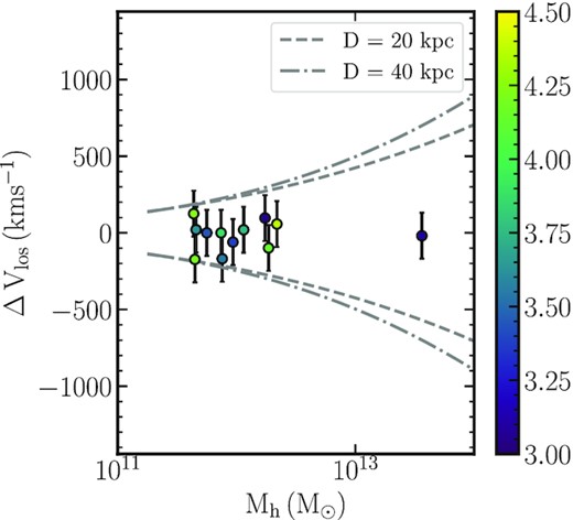
The velocity difference between the Mg ii absorbing gas along the quasar sightline and the USMg ii host galaxies is plotted against their dark matter halo mass colour coded following |$\rm {\mathit{ W}_{2796}}$| as indicated on the right side of the figure. The grey dashed and dot–dashed lines correspond to the escape velocity for the dark matter halo potential at the impact parameters of 20 and 40 kpc, respectively. For each measured velocity difference, we associate an error bar of ±150 km s−1.
However, in order to quantify what fraction of the absorbing gas is bound to the galaxy we also need to know the line of sight velocity spread. Recall that a large W2796 of USMg ii absorption will correspond to large velocity spread, Δvlos, along our line of sight (see Ellison 2006; Zou et al. 2018). It is well known that W2796 is strongly correlated with Δvlos. This correlation will imply Δvlos > 300 km s−1for our sample. It is also suggested that velocity widths in excess of 300 km s−1 may originate from multiple components (see e.g. Ledoux et al. 1998; Zou et al. 2018). As mentioned before, in three systems in our sample we see multiple component structure even at SDSS resolution. Also in three cases we see more than one galaxy at the same redshift as the USMg ii absorber. The errorbars in Fig. 15 indicate a spread of ±150 km s−1 around the measured velocity offset. If velocity spreads are of this order then in most cases the absorbing gas will be bound to the galaxy. However, high resolution spectroscopic observations are needed to directly measure the fraction of absorbing gas bound to the galaxies.
6.2 Are USMg ii host galaxies starbursts?
To investigate whether the USMg ii host galaxies identified in our sample are regular star-forming galaxies, or star-burst or post star-burst galaxies, we put these galaxies in the SFR scaled by the main-sequence SFR at the redshift of the galaxy (Speagle et al. 2014) versus stellar mass plot as shown in Fig. 16. In the same plot, we have also shown the isolated Mg ii absorbers within the impact parameter of 60 kpc from the magiicat sample. We identify that the USMg ii host galaxies have systematically less SFR (i.e median SFR = 0.6 SFRMS) compared to the star-forming main sequence (Speagle et al. 2014) as well as the magiicat host galaxies (median SFR = 1.5 SFRMS). Thus USMg ii systems considered here are not star bursting galaxies and typically form stars at a rate slightly lower than the star-forming main sequence.

Scatter plot of SFR scaled by the SFR of a main-sequence galaxy of the same stellar mass at zabs (SFRMS) versus stellar mass for USMg ii (circle) and magiicat host galaxies (squares). Color coding is based on the rest equivalent width, |$\rm {\mathit{ W}_{2796}}$|. The black solid line corresponds to SFR of the main sequence. The dashed black line corresponds to the median SFR of the magiicat galaxies while the dot–dashed line corresponds to that of the USMg ii host galaxies.
6.3 Fraction of galaxies producing USMgII absorption
From Fig. 10, we see that USMg ii host galaxies can have impact parameters up to 40 kpc. However, only a fraction of galaxies within D ∼ 40 kpc will produce an USMg ii absorption. To find this fraction (|$f_{\mathrm{ USMg}\small {\rm II}}$|), we consider the isolated galaxies in galaxycentric Mg ii absorption surveys conducted by Dutta et al. (2020), Huang et al. (2021), and also the magiicat. We find only one out of 34 galaxies (i.e. |$f_{\mathrm{ USMg}\small {\rm II}}\sim 0.03$|) at D ≤ 20 kpc and none of the 106 galaxies at 20 ≤ D(kpc) ≤ 40 produce USMg ii absorption. For the full range, D ≤ 40, we get an average |$f_{\mathrm{ USMg}\small {\rm II}} \sim 0.007$|. Usually, |$f_{\mathrm{ USMg}\small {\rm II}}$| values are interpreted in terms of covering factor of the gas. In this picture, the projected area around galaxy centres covered by the USMg ii absorber is ∼1 per cent of the total area. The large W2796 seen in the USMg ii absorbers suggest large velocity spread among multiple clouds along our line of sight.
Another possible interpretation of low |$f_{\mathrm{ USMg}\small {\rm II}}$| is to say USMg ii originate from a different population of galaxies.
The impact parameter distribution of USMg ii host galaxies not following the general population (see Section 5.4) may suggest that USMg ii selection picks a different population (high M⋆ with relatively low SFR/SFRMS and low ionization parameter with large reservoir of CGM gas) of host galaxies.
6.4 Galaxy environments of USMg ii absorbers
From the recent studies (Fossati et al. 2019; Dutta et al. 2020; Hamanowicz et al. 2020) of Mg ii absorption systems with integral field units (IFU) like MUSE, there is growing evidence that a significant fraction of Mg ii absorbing gas might not be associated with isolated galaxies. As mentioned before, there is one USMg ii system present in the sample of Dutta et al. (2020) and three in the sample of Schroetter et al. (2019). Interestingly, for all these 4 systems the host galaxies are found to be isolated (i.e. no other galaxy is found within 100 kpc from the quasar sightline and a maximum velocity separation of 500 |$\mathrm{ km}\, \mathrm{ s}^{-1}$|). As discussed in Section 3.1, there are 7 USMg ii absorbers with only one potential host galaxy (with mr < 23.6 mag) within an impact parameter of 100 kpc. Therefore, at least 33 per cent of USMg ii absorbers in our sample are hosted by isolated galaxies. This fraction is 57 per cent if we consider the limiting magnitude of mr = 22.5 mag. We identify three cases (i.e ∼14 per cent) that are likely to be associated with more than one galaxy. These systems are towards J0156+0343, J2207−0901, and J2338−0056. For the first case (J0156+0343), we detect extended [O ii] emission consistent with the host galaxy(ies) being part of merging systems (see Fig. 5). The second case (J2207−0901) has already been studied by Gauthier (2013) and the USMg ii absorption is likely to be originating from intragroup gas. For the third system (J2338−0056), we identify a USMg ii host galaxy at an impact parameter of 79 kpc, however, there are two more galaxies (with consistent photometric redshift) present for which we could not get the spectrum and these are likely to be part of a galaxy group.
7 CONCLUSIONS
In this paper, we have explored the nature of the galaxies hosting USMg ii absorption at redshift, z ∼ 0.5. Main summary of this work is provided below.
Using the SDSS Mg ii/Fe ii absorber catalog (Zhu & Ménard 2013), we have created a sample of 109 USMg ii absorbers accessible to SALT in the redshift range 0.4 ≤ zabs ≤ 0.6. From this sample, we confirm only 27 absorbers to be USMg ii systems. Out of these 27 systems, 21 of them were observed with SALT and for 18 of them, the USMg ii host galaxies are identified. Among the rest of the 5 unobserved systems, two of them are GOTOQs, i.e, emission is detected in the background quasar spectra. Therefore, among the 27 USMg ii systems, we have identified the host galaxies for 20 of them.
Given the power-law fit (Chen et al. 2010a) between the impact parameter (D) and the rest equivalent width (|$\rm {\mathit{ W}_{2796}}$|), one expects the USMg ii absorbers to reside within D ∼ 5 kpc. However, for our sample, the impact parameters ranges from 7.3 to 79 kpc with a median of 18 kpc. Using the log-linear fit to the combined sample (Nielsen et al. 2013a), we argue that the USMg ii absorbers constitute statistically distinct population in the W2796–D plane.
Among the 23 USMg ii systems (20 detections and 3 non-detections), we have detected [O ii] emission in 18 cases. We conclude that, including the two unobserved GOTOQs, about 70 per cent of the host galaxies are star forming (i.e SFR ≥ 1 M⊙ yr−1). The measured [O ii] luminosities are in the range of |$0.06 L_{[\mathrm{ O}\,\small {\rm II}]}^\star$| to |$1.43 L_{[\mathrm{ O}\,\small {\rm II}]}^\star$| with a median value of |$0.39 L_{[\mathrm{ O}\,\small {\rm II}]}^{\star }$|.
When we combined our sample with those from the literature, we find a positive correlation between W2796 and |$L_{{[\mathrm{ O}\,\ {\small{\rm II}}]}}$| (rS = 0.34 and p-value of <10−4) for USMg ii host galaxies as well as from the literature (see Fig. 12). However, this correlation is seen to be driven by weak Mg ii absorbers (i.e W2796 < 1 Å) which tend to be associated with low luminosity galaxies with higher D.
Compared to the field galaxies and the GOTOQs, we find the measured emission lines ratios [O iii]/[O ii] and [O iii]/|$\rm {H\,\beta }$| to be smaller for the USMg ii host galaxies. Using photoionization models we find this trend to be driven by the ionizing radiation in these USMg ii host galaxies being softer compared to the field galaxies.
We measure galaxy parameters like, stellar mass (10.21 ≤ log [M⋆/M⊙] ≤ 11.62), B-band magnitude (−21.68 ≤ MB ≤ −19.05), star formation rate (2.59 ≤ SFR[M⊙yr−1] ≤ 33.51) and halo mass (11.64 ≤ log [Mh/M⊙] ≤ 13.56) using SED fitting. The inferred virial radius of haloes (145 ≤ Rh[kpc] ≤ 624) are at least 5 times larger than the impact parameter measured. The measured M⋆ for USMg ii are higher than those found for general Mg ii absorbers at a given impact parameter. However the measured SFRs are slightly lower than what has been predicted by star-forming main sequence.
The general population of Mg ii absorbers show a correlation between D and M⋆. We find the USMg ii systems to not follow this trend. For the same impact parameter, the USMg ii host galaxies are more massive and luminous compared to the host galaxies of relatively weak Mg ii absorbers.
We find the mean velocity difference between the Mg ii absorption redshift and galaxy redshift from [O ii] emission to μ = 3.48 ± 5.82 km s−1 with a σ = 71.02 ± 4.83 km s−1. This velocity difference is well within the expected escape velocities for the inferred range of Mh. However, we argue that W2796 measured along the line of sight should correspond to a velocity width in excess of 300 km s−1. Therefore, what fraction of the observed gas in USMg ii systems is bound can be answered only using high resolution spectra. Additionally, large velocity widths could indicate multiple components (i.e merging systems) contributing to the absorption. This can also be probed using high-resolution spectroscopy.
In the literature sample of USMg ii systems we find all the 4 known host galaxies are isolated (no companion galaxy within 100 kpc and ±500 km s−1). In our sample we find that at least |$33{{\ \rm per\ cent}}$| of host galaxies of USMg ii are isolated up to a projected distance of 100 kpc and the r-band limiting magnitude of 23.6. Measuring the galaxy orientations using high spatial resolution imaging of the isolated galaxies together with a high-SNR spectrum probing the down the barrel absorption will be very useful to quantify the role of strong outflows in the case of USMg ii systems.
SUPPORTING INFORMATION
Figure A1. Gaussian fits to absorption profiles of Mn ii, Fe ii, Mg ii, and, Mg i for the all USMg ii systems in our sample in the rest frame of the absorbing gas.
Figure A2. Gaussian fit to the Ca ii absorption associated with the USMg ii absorptions in the absorber rest frame.
Figure D1. Ca ii λ 3935 rest equivalent width plotted against the color excess of the background quasars for our USMgii sample (blue), high redshift C ii absorbers (orange) (Zou et al. 2018), and the Ca ii absorbers from SDSS DR3 in the redshift range 0.84 ≤ zabs ≤ 1.3 (Wild & Hewett 2005).
Figure E1. L|$_{[\rm \mathrm{ O}\,\, {\small{\rm III}}]}$|/L|$_{[\rm O\, {\small{\rm II}}]}$| ratio vs the rest equivalent width of Mg ii for both GOTOQs (orange) and our USMgii (blue) sample.Green stars give median values of the ratio for different W2796 bins.
Figure G1. The figure shows the plot of W2796 against the impact parameter D for absorbers at 0.4 ≤ z ≤ 0.6 in different samples.
Figure G2. W2796 versus the impact parameter for the USMg ii host galaxies from our sample (red) as well as from the literature (blue).
Figure H1. Absolute B-band magnitude of the Mg ii host galaxies plotted against the impact parameter.
Table B1. Details of all the 109 USMg ii absorber from Zhu & Ménard (2013).
Table C1. Details of galaxies with consistent photo-z to the USMgii absorbers in our sample with D < 100 kpc.
Table F1. Details of USMg ii from the literature.
Please note: Oxford University Press is not responsible for the content or functionality of any supporting materials supplied by the authors. Any queries (other than missing material) should be directed to the corresponding author for the article.
ACKNOWLEDGEMENTS
All the new observations reported in this paper were obtained with the Southern African Large Telescope (SALT). RD gratefully acknowledges support from the European Research Council (ERC) under the European Union’s Horizon 2020 research and innovation programme (grant agreement No 757535). This project makes use of the following softwares : NumPy (Harris et al. 2020), SciPy (Virtanen et al. 2020), Matplotlib (Hunter 2007), and AstroPy (Astropy Collaboration et al. 2013, 2018). LKG thanks Aromal P for helpful discussions on data reductions and data analysis.We thank the anonymous referee for the comments and suggestions that significantly improved the presentations of this paper.
This paper makes use of SDSS observational data. Funding for the Sloan Digital Sky Survey IV has been provided by the Alfred P. Sloan Foundation, the U.S. Department of Energy Office of Science, and the Participating Institutions. SDSS-IV acknowledges support and resources from the Center for High Performance Computing at the University of Utah. The SDSS website is www.sdss.org. SDSS-IV is managed by the Astrophysical Research Consortium for the Participating Institutions of the SDSS Collaboration including the Brazilian Participation Group, the Carnegie Institution for Science, Carnegie Mellon University, Center for Astrophysics | Harvard & Smithsonian, the Chilean Participation Group, the French Participation Group, Instituto de Astrofísica de Canarias, The Johns Hopkins University, Kavli Institute for the Physics and Mathematics of the Universe (IPMU) / University of Tokyo, the Korean Participation Group, Lawrence Berkeley National Laboratory, Leibniz Institut für Astrophysik Potsdam (AIP), Max-Planck-Institut für Astronomie (MPIA Heidelberg), Max-Planck-Institut für Astrophysik (MPA Garching), Max-Planck-Institut für Extraterrestrische Physik (MPE), National Astronomical Observatories of China, New Mexico State University, New York University, University of Notre Dame, Observatário Nacional / MCTI, The Ohio State University, Pennsylvania State University, Shanghai Astronomical Observatory, United Kingdom Participation Group, Universidad Nacional Autónoma de México, University of Arizona, University of Colorado Boulder, University of Oxford, University of Portsmouth, University of Utah, University of Virginia, University of Washington, University of Wisconsin, Vanderbilt University, and Yale University.
DATA AVAILABILITY
Data used in this work are obtained using SALT. Raw data will become available for public use 1.5 yr after the observing date at https://ssda.saao.ac.za/.
