-
PDF
- Split View
-
Views
-
Cite
Cite
Matteo Cataneo, Cora Uhlemann, Christian Arnold, Alex Gough, Baojiu Li, Catherine Heymans, The matter density PDF for modified gravity and dark energy with Large Deviations Theory, Monthly Notices of the Royal Astronomical Society, Volume 513, Issue 2, June 2022, Pages 1623–1641, https://doi.org/10.1093/mnras/stac904
Close - Share Icon Share
ABSTRACT
We present an analytical description of the probability distribution function (PDF) of the smoothed 3D matter density field for modified gravity and dark energy. Our approach, based on the principles of Large Deviations Theory, is applicable to general extensions of the standard Lambda cold dark matter (ΛCDM) cosmology. We show that late-time changes to the law of gravity and background expansion can be included through Einstein-de Sitter spherical collapse dynamics combined with linear theory calculations and a calibration measurement of the non-linear variance of the smoothed density field from a simple numerical simulation. In a comparison to N-body simulations for f(R), DGP, and evolving dark energy theories, we find per cent level accuracy around the peak of the distribution for predictions in the mildly non-linear regime. A Fisher forecast of an idealized experiment with a Euclid-like survey volume demonstrates the power of combining measurements of the 3D matter PDF with the 3D matter power spectrum. This combination is shown to halve the uncertainty on parameters for an evolving dark energy model, relative to a power spectrum analysis on its own. The PDF is also found to substantially increase the detection significance for small departures from General Relativity, with improvements of up to six times compared to the power spectrum alone. This analysis is therefore very promising for future studies including non-Gaussian statistics, as it has the potential to alleviate the reliance of these analyses on expensive high-resolution simulations and emulators.
1 INTRODUCTION
Over the past two decades an extraordinary and diverse array of experimental evidence has earned the Lambda cold dark matter (ΛCDM) paradigm the status of standard cosmological model (see e.g. Aiola et al. 2020; Hamana et al. 2020; Planck Collaboration VI 2020; Alam et al. 2021; DES Collaboration 2022; Dutcher et al. 2021; Heymans et al. 2021, for recent analyses). However, in recent years mild to severe tensions between early- and late-time probes of the growth of structure and background expansion have put a strain on the ability of ΛCDM to explain our universe (see e.g. Douspis, Salvati & Aghanim 2019; Di Valentino et al. 2021a,b; Perivolaropoulos & Skara 2021, for reviews). Furthermore, Einstein’s general relativity (GR) – the theory of gravity at the foundation of ΛCDM – has been thoroughly tested only on small astrophysical scales and in the strong field regime (Will 2014; Abbott et al. 2017, 2019b), leaving ample room for modifications to the field equations on cosmological scales (Abbott et al. 2019a; Ferreira 2019; Ishak 2019; Pogosian et al. 2021; Raveri et al. 2021; Tröster et al. 2021). Together with the yet unexplained nature of the observed accelerated cosmic expansion (Riess et al. 1998; Perlmutter et al. 1999), these considerations motivate the exploration of alternatives to the cosmological constant (Λ) and standard gravity. In this paper, we focus on extensions of ΛCDM that include modified gravity and (late-time) dark energy, which we will concisely refer to as ‘extended models’.
Two-point statistics are central to many of the leading cosmological analyses of the large-scale structure searching for deviations from ΛCDM (Simpson et al. 2013; Song et al. 2015; Amon et al. 2018; Abbott et al. 2019a; Chudaykin, Dolgikh & Ivanov 2021; Lee et al. 2022; Muir et al. 2021; Tröster et al. 2021; Vazsonyi et al. 2021), and a great deal of effort has gone into accurately modelling the non-linear matter power spectrum in modified gravity and dark energy cosmologies – a theoretical ingredient essential to extract the cosmological information locked in small scales (e.g. Koyama, Taruya & Hiramatsu 2009; Brax & Valageas 2012; Takahashi et al. 2012; Heitmann et al. 2014; Zhao 2014; Casarini et al. 2016; Mead et al. 2016; Cusin, Lewandowski & Vernizzi 2018; Cataneo et al. 2019; Winther et al. 2019; Euclid Collaboration 2021; Ramachandra et al. 2021). However, non-linear gravitational clustering converts the nearly Gaussian initial density field (Planck Collaboration VI 2020) to a late-time density field with significant non-Gaussian features that these standard analyses are unable to access (Bernardeau et al. 2002). Non-Gaussian statistics, such as the bispectrum (Brax & Valageas 2012; Munshi 2017; Yamauchi, Yokoyama & Tashiro 2017; Crisostomi, Lewandowski & Vernizzi 2020; Bose et al. 2020b), higher order weak lensing spectra (Munshi & McEwen 2020), the halo mass function (Lam & Li 2012; Cataneo et al. 2016; Hagstotz et al. 2019; McClintock et al. 2019; Bocquet et al. 2020), the void size function (Perico et al. 2019; Verza et al. 2019; Contarini et al. 2021) and Minkowski functionals (Kratochvil et al. 2012; Fang, Li & Zhao 2017), respond strongly to modified gravity and dark energy through the induced changes in the higher moments of the cosmic density field, and their remarkable complementarity to traditional two-point functions leads to tighter joint constraints on the extra non-standard parameters (Shirasaki et al. 2017; Peel et al. 2018; Sahlén 2019; Liu et al. 2021).
The probability distribution function (hereafter PDF) of the 3D matter density field smoothed on a given scale is one of the simplest non-Gaussian statistics, and accurate predictions allow us to extract additional cosmological information (Uhlemann et al. 2020). Modified gravity and evolving dark energy leave distinctive imprints on the skewness, kurtosis, and higher cumulants of the PDF, which have been observed in N-body simulations (Li, Zhao & Koyama 2012b; Hellwing et al. 2013, 2017; Shin et al. 2017). Thus far, theoretical predictions of the PDF for modified gravity have required either sophisticated and time-consuming approaches for the spherical collapse (Brax & Valageas 2012) or computationally costly simulations (Li et al. 2012b; Hellwing et al. 2013, 2017). Similarly, for the PDF response to dark energy beyond a cosmological constant, so far only ad hoc fitting functions obtained from simulations are available (Shin et al. 2017; Mandal & Nadkarni-Ghosh 2020; Wen, Kemball & Saslaw 2020). In this work, we apply the principles of Large Deviation Theory (LDT) to the cosmic density field to derive a general and analytical prescription for the 3D matter PDF in modified gravity and dark energy cosmologies. We build on the formalism developed in Bernardeau & Reimberg (2016) and Uhlemann et al. (2016), and show that the Einstein-de Sitter (EdS) spherical collapse dynamics together with linear theory calculations can reproduce the 3D matter PDF measured from state-of-the-art simulations to a few per cent accuracy in the mildly non-linear regime. Remarkably, the matter PDF can be accurately predicted requiring only linear information from extended cosmologies, which sources the characteristic differences in the non-linear variance and higher cumulants. Through Fisher forecasts we quantify, for the first time, the ability of the PDF to detect distinct departures from GR and to constrain the dark energy equation of state, especially when combined with the matter power spectrum. Our method implemented in the public code pyLDT1 delivers fast predictions for the cosmology dependence of the PDF, and it paves the way for the modelling of observable statistics of the large-scale structure in general theories of gravity and dark energy (see Frusciante & Perenon 2020, for a review). Our framework can be applied to predict the weak lensing convergence PDF (Barthelemy et al. 2020; Boyle et al. 2021), galaxy counts-in-cells (Uhlemann et al. 2018a; Repp & Szapudi 2020; Friedrich et al. 2022), and density-split statistics (Friedrich et al. 2018; Gruen et al. 2018).
The paper is structured as follows: Section 2 reviews the LDT framework and provides a simple extension to include the effects of modified gravitational couplings and background expansion on the PDF. Section 3 describes the N-body simulations and PDF measurements used to validate the theoretical predictions. In Section 4, we demonstrate the accuracy of our methodology, as well as the complementarity of the matter PDF and the power spectrum for modified gravity and dark energy parameters using Fisher matrix analyses. We summarize our results and give an outlook on future research in Section 5.
2 THE MATTER DENSITY PDF IN LARGE DEVIATIONS THEORY
2.1 Large deviations theory framework
Remarkably, for a standard ΛCDM universe, there are only three ingredients that enter this theoretical model for the matter PDF,
the time- and scale-dependence of the linear variance, |$\sigma _{\rm L}^2(r,z)$|,
the mapping from initial to final densities in spheres, ρSC(δL),
the non-linear variance of the log-density at the sphere radius and redshift of interest, |$\sigma _{\rm NL}^2(R,z) \rightarrow \sigma _{\mu }^2(R,z)$| .
The linear variance and its cosmology dependence can be readily obtained from the linear power spectrum computed from Einstein–Boltzmann codes like CAMB (Lewis, Challinor & Lasenby 2000) or CLASS (Blas, Lesgourgues & Tram 2011).
The spherical collapse mapping entering the matter PDF was shown to be very mildly cosmology-dependent and well-approximated by the redshift-independent EdS result in Uhlemann et al. (2020). This can also be seen in Fig. 1, where the fractional difference between the ΛCDM and the EdS solution remains within 0.25 per cent for all non-linear densities considered. We develop a simple yet accurate EdS-based approximation for spherical collapse within modified gravity in the following section.
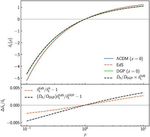
Mapping between the normalized final density, ρ, and the initial linearly scaled density fluctuation, δL, for a spherical top-hat perturbation. Upper panel: the curves show the density evolution in different background/gravity models. For ΛCDM (blue) and EdS (dashed orange) cosmologies gravity is GR, while for DGP (green) the gravitational constant is modified as in equation (11) with rcH0 = 0.5 (or Ωrc = 0.25). Here, both ΛCDM and DGP are evaluated at z = 0. The dashed black line represents the EdS mapping rescaled by the ratio of the ΛCDM-to-DGP linear growth ratio at z = 0. Lower panel: fractional difference of the EdS mapping from the ΛCDM prediction (dashed orange) and that of the rescaled EdS from the DGP evolution (dashed black). The rescaled |$\delta _{\rm L}^{\rm EdS}$| can reproduce the modified gravity phenomenology to better than 0.5 per cent, and it can be seen that most of the difference comes from the discrepancy between the EdS and the ΛCDM predictions.
The non-linear variance of the log-density at the sphere radius and redshift of interest, |$\sigma _{\mu }^2(R,z)$|, can be considered a free parameter and measured directly from simulations. Once measured from a single (or small set of) simulations at the fiducial cosmology, its changes with cosmology can be predicted using a phenomenological approximation inspired from the lognormal model (see equation 21). Alternatively, the non-linear variance of the log-density could also be chosen to reproduce a predicted non-linear variance of the density, |$\sigma _{\rho }^2(R,z)$|, obtained from matter power spectrum fitting functions such as halofit (Peacock & Smith 2014), hmcode (Mead et al. 2021), or respresso (Nishimichi, Bernardeau & Taruya 2017).
2.2 Large-deviations statistics in modified gravity and dark energy
2.2.1 Modified gravity
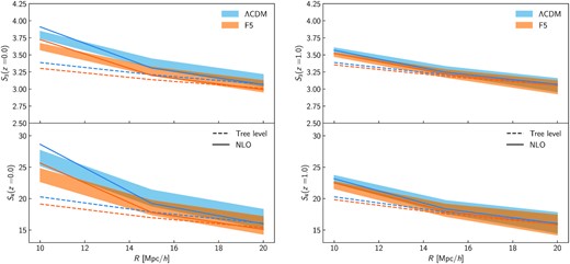
Reduced cumulants associated with skewness (top) and kurtosis (bottom) of the smoothed matter density PDF at z = 0 (left) and z = 1 (right) for ΛCDM (blue) and f(R) gravity with |fR0| = 10−5 and n = 1 (orange). For each smoothing radius, R = 10, 15, 20 |$\mathrm{Mpc}\, h^{-1}$|, the coloured bands represent the mean and error on the mean across 8 N-body realizations, and the lines correspond to the theoretical predictions. Solid lines are computed with the tree-level approximation and dashed lines use the next-to-leading order (NLO) correction equation (18), with all vertices derived from the EdS spherical collapse dynamics. The cosmology dependence and modified gravity effects are mostly sourced by the linear variance, while the non-linear variance contributes only to a minor extent.
Baseline ΛCDM cosmological parameters for the three simulation suites used in this work. The first column refers to the extension investigated within that particular suite. Ωm and Ωb are, respectively, the present-day background total matter and baryon density in units of the critical density, h = H0/100 is the dimensionless Hubble constant, As and ns are the amplitude and slope of the primordial power spectrum, and |$\sigma _8^\Lambda$| is the amplitude of mass fluctuations for the baseline ΛCDM cosmology.
| . | Ωm . | Ωb . | h . | ns . | As × 109 . | |$\sigma _8^\Lambda$| . |
|---|---|---|---|---|---|---|
| DGP | 0.3072 | 0.0481 | 0.68 | 0.9645 | 2.085 | 0.821 |
| f(R) | 0.31315 | 0.0492 | 0.6737 | 0.9652 | 2.097 | 0.822 |
| DE | 0.26 | 0.044 | 0.72 | 0.96 | 2.082 | 0.79 |
| . | Ωm . | Ωb . | h . | ns . | As × 109 . | |$\sigma _8^\Lambda$| . |
|---|---|---|---|---|---|---|
| DGP | 0.3072 | 0.0481 | 0.68 | 0.9645 | 2.085 | 0.821 |
| f(R) | 0.31315 | 0.0492 | 0.6737 | 0.9652 | 2.097 | 0.822 |
| DE | 0.26 | 0.044 | 0.72 | 0.96 | 2.082 | 0.79 |
Detection significance for a fiducial f(R) gravity model with |fR0| = 10−6, and a fiducial DGP model with Ωrc = 0.0625. The constraints on f(R) gravity from the PDF are stronger than in DGP owing to the additional skewness produced by the scale-dependent fifth force, which is visible in the |fR0| derivatives shown in Fig. 11. Moreover, unlike DGP, where the approximate theory PDF matches the ΛCDM prediction at z = 0, in f(R) gravity the PDF differs from that of the standard cosmology at low redshifts, which allows even more non-linear information to be extracted.
| . | F6 detection . | DGPw detection . |
|---|---|---|
| PDF, 3 scales + prior | 5.15σ | 1.17σ |
| P(k), |$k_{\rm max} = 0.2\ h \,\rm Mpc^{ -1}$| + prior | 2.01σ | 2.42σ |
| PDF + P(k) + prior | 13.40σ | 5.19σ |
| . | F6 detection . | DGPw detection . |
|---|---|---|
| PDF, 3 scales + prior | 5.15σ | 1.17σ |
| P(k), |$k_{\rm max} = 0.2\ h \,\rm Mpc^{ -1}$| + prior | 2.01σ | 2.42σ |
| PDF + P(k) + prior | 13.40σ | 5.19σ |
Constraints from mildly non-linear scales on σ8, w0, and wa derived including a prior on {Ωb, ns}, as well as dark energy Figure of Merit (FoM) for the matter PDF, power spectrum and their combination.
| . | |$\frac{\sigma [\sigma _8]}{\sigma _8^{\rm fid}}$| . | σ[w0] . | σ[wa] . | FoM . |
|---|---|---|---|---|
| PDF, 3 scales + prior | 0.18 per cent | 0.37 | 1.25 | 27 |
| |$P(k), k_{\rm max}=0.2 \, h\, \mathrm{Mpc}^{-1}$| + prior | 0.45 per ent | 0.24 | 1.03 | 50 |
| PDF + P(k) + prior | 0.17 per cent | 0.09 | 0.40 | 243 |
2.2.2 Evolving dark energy
The non-linear growth of spherical top-hat fluctuations is also affected by the evolving dark energy density via the Hubble parameter in equation (8). However, we follow the approach proposed by Codis et al. (2016) (i.e. keeping the spherical evolution fixed as in EdS) and compute the matter PDF by means of equation (19). We quantify a posteriori the goodness of this choice by comparing our predictions against state-of-the-art cosmological simulations in Section 4.
2.2.3 pyLDT
We have implemented the large-deviation theory predictions described in Section 2.1 together with equations (19) in pyLDT, a modularized and user-friendly python code that takes advantage of the PyJulia interface for computationally intensive tasks. The linear growth for f(R) gravity and DGP is obtained by solving equation (6), while the linear power spectrum for the standard cosmology, as well as for the evolving dark energy models, is computed with camb8 (Lewis et al. 2000). Extensions to other modified gravity theories only require either to add a specific function describing changes to the gravitational constant, ϵ(k, a), or to couple the code to dedicated Einstein–Boltzmann solvers such as hi_class (Zumalacárregui et al. 2017; Bellini, Sawicki & Zumalacárregui 2020) and EFTCAMB (Hu et al. 2014).
3 SIMULATIONS
3.1 f(R) gravity simulations
The initial conditions (ICs) of the independent realizations were selected such that the large-scale sample, or cosmic, variance in the 3D matter power spectrum is minimal when averaged over the simulations. In order to implement this we created 100 independent initial conditions using 2lptic (Crocce, Pueblas & Scoccimarro 2006) and measured their 3D matter power spectrum. We then considered all possible pairs of these ICs and selected the four ‘best’ pairs according to the following criteria (this follows the procedure outlined in Harnois-Deraps, Giblin & Joachimi 2019 to find ICs with approximately opposite modes on large scale):
each individual power spectrum of a selected pair, as well as their average power spectrum, should deviate as little as possible from the desired linear theory power spectrum for k < kNy/2 = πNp/2Lbox;
and the relative difference of each individual power spectrum to the theory spectrum should fluctuate around zero on large scales rather than being positive or negative over large k-ranges to avoid a leakage of power from large to small scales.
To simulate structure formation in f(R) gravity the simulation code has to solve both the standard Newtonian forces and the fifth force. arepo computes the standard gravity forces using a Tree Particle-Mesh algorithm in our simulations. The f(R) gravity forces are computed employing an iterative solver on an adaptively refining mesh which ensures increased resolution in high-density regions (see Arnold et al. 2019, for details).
Due to the very non-linear behaviour of the scalar field in f(R) gravity, tracking its evolution is computationally very expensive. To keep the computational cost of the simulations as small as possible, arepo therefore employs an adaptive timestepping scheme which only updates the MG forces when necessary (Arnold et al. 2019). The standard gravity accelerations are largest (and change most frequently) within large haloes, so that they have to be updated with a very small time-step. However, these very same regions in f(R) gravity are largely screened for |fR0| ≲ 10−5. Therefore, the maximum MG acceleration will typically be much smaller than the maximum standard gravity acceleration, allowing a larger MG time-step without compromising the accuracy of the simulations.
3.2 DGP simulations
The DGP simulations used in this work were first presented in Cataneo et al. (2019), and they were carried out using the ecosmog code (Li, Zhao & Koyama 2013; Li et al. 2012a), which is based on the publicly available Newtonian cosmological N-body and hydrodynamical simulation code ramses (Teyssier 2002). This code solves the non-linear equation of motion of the scalar field in the DGP model using adaptively refined meshes, where a cell in the mesh splits into 8 son cells when the effective particle number of simuation particles in it exceeds 8. We have run one realization with box size Lbox = 512 Mpc h−1 and particle number Np = 10243 for each of the following: a baseline ΛCDM cosmology with cosmological parameters listed in Table 1, two DGP models with Ωrc = 0.25 (DGPm) and Ωrc = 0.0625 (DGPw), and the corresponding pseudo cosmologies with final output redshifts zf = 0 and zf = 1. These runs adopt a domain grid, i.e. a regular base grid with uniform resolution that covers the entire simulation domain, with 10243 cells. Although it has been shown that, for many of the usual statistics of matter and dark matter halo fields, very fine simulation meshes are not necessary for the DGP model (Barreira, Bose & Li 2015), in these runs we have not set an upper limit of the highest refinement level, given that they were designed to be used to study novel statistics. At late times, the most refined regions in the simulation domain have a cell size that is 1/26 times the domain grid cell size; this corresponds to an effective force resolution (twice the cell size) of ≃ 15.3 kpc h−1 in those regions.
The ICs of these simulations are again generated using 2lptic, with an initial redshift zini = 49. This is lower than the initial redshift used for the f(R) runs described above (zini = 127), but the second-order Lagrangian perturbation theory is still a good approximation at z = 49. Since the effect of modified gravity is negligible at z > 49, it is neglected in the ICs.
3.3 Evolving dark energy simulations
For the evolving dark energy cosmologies we used the publicly available matter density PDFs9 measured from a suite of single-realization N-body simulations with Np = 20483 and Lbox = 1024 |$\mathrm{Mpc}\, h^{-1}$| described in Shin et al. (2017). The baseline flat ΛCDM cosmology has the parameters listed in Table 1, and for the w0waCDM cosmologies we have the four pairs {w0, wa} = { − 1.5, 0}, { − 0.5, 0}, { − 1, −1}, and { − 1, +1}. The power spectrum normalization at z = 0 is fixed to its baseline value for all dark energy extensions except for {w0, wa} = { − 1, +1}, which we found to have a somewhat smaller σ8.10
3.4 PDF measurements from the simulations
For our f(R) gravity, DGP and corresponding pseudo and ΛCDM simulations we measured the PDFs of the smoothed matter density field as follows. First, for each snapshot we reconstruct the continuous density field using the Delaunay Tassellation Field Estimator method (Schaap & van de Weygaert 2000) and sample it over a 10243 mesh, all of which is automatically performed by the public code dtfe11 (Cautun & van de Weygaert 2011). Next, we convolve the sampled density field with spherical top-hat filters of radii R = 10, 15, and 20 |$\mathrm{Mpc}\, h^{-1}$| (an operation we do in Fourier space). Lastly, we construct the PDF by collecting the normalized density values, ρR = 1 + δR, in 99 logarithmically spaced bins in the range [0.01,100]. In Appendix A, we show that this method produces PDFs in excellent agreement with those obtained by applying the Cloud-in-Cell (CiC) mass assignment scheme. We report variances and means extracted from the simulations for both the density and the log-density fields in Appendix B.
For the DE simulation suite, instead, the smoothed density field was obtained by summing over the mass of all the particles contained in spheres centred at the 20483 nodes of a regular grid and dividing by the volume of the spheres. In this work, we consider the PDFs measured in spheres of radius R = 10 and 25 |$\mathrm{Mpc}\, h^{-1}$| for the z = 0, 0.5, and 1 snapshots.
4 RESULTS
In the following, we first present our results for the modified gravity and dark energy cosmologies discussed in Section 2.2, and then examine the detection potential of departures from ΛCDM for idealized statistical analyses combining the full shape of the PDF and the matter power spectrum.
4.1 Modified gravity
As discussed in Section 2.2, on mildly non-linear scales the EdS dynamics approximates well the evolution of spherical top-hat density fluctuations even in cosmologies where the law of gravity deviates substantially from GR. Here, by using state-of-the-art simulations we assess how such an approximation impacts the accuracy of the LDT predictions for the matter PDF in two specific modified gravity scenarios, DGPm and F5 (see Section 3 for details). Equivalent results for DGPw and F6 can be found in Appendix C.
Fig. 3 shows how the global shape of the PDF responds to scale-independent (left) or scale-dependent (right) modifications to the linear growth. As expected, when sharing the same initial conditions with ΛCDM both PDFs approach the standard result at high redshifts and exhibit their largest deviations at low redshifts, and do so at a rate specific to the model under consideration. However, there are clear differences that reflect the infinite or finite range of the fifth force. In DGP, structures on all scales are subject to the same modification, and changes to the higher moments of the distribution are mainly driven by increases in the variance. This follows immediately from the expressions for the reduced cumulants in equation (18) – where the tree-level terms are identical for DGP and ΛCDM – and will be explored in more detail below. In f(R) gravity, instead, density fluctuations evolve in different gravity conditions depending on their size. For example, the present-day Compton wavelength in our F5 cosmology is approximately 8 |$\mathrm{Mpc}\, h^{-1}$| (and smaller at earlier times). Therefore, spherical overdensities reaching a final radius R = 10 |$\mathrm{Mpc}\, h^{-1}$| experience very little fifth force for most of their collapse history. In contrast, spherical underdensities have sizes comparable to or smaller than the Compton wavelength (at the same epoch) and thus experience the fifth force in the later stages of their expansion (i.e. z ≲ 2), with the emptiest regions experiencing a full 33 per cent enhancement of the gravitational force. It is this asymmetric behaviour that contributes to the increased skewness of the PDF in f(R) gravity compared to ΛCDM (see also Hellwing et al. 2013), our model equation (19) can capture it thanks to the linear variance term probing different scales, r = Rρ1/3, depending on the density of the sphere, ρ (see also equation 4).

Matter PDF in spheres of radius R = 10 |$\mathrm{Mpc}\, h^{-1}$| at z = 0 (blue) and z = 1 (green) for ΛCDM (dashed) and modified gravity (solid). Left: Data points are the simulation measurements from a single realization (triangles for ΛCDM and squares for DGPm) and lines represent the theory predictions. For DGP the primary effect of the enhanced growth is that of increasing the variance of the distribution, which in turn results in heavier tails, i.e. more under/overdense structures compared to the standard cosmology. Right: data points and corresponding uncertainties are the mean and error on the mean measured from 8 realizations (triangles for ΛCDM and squares for F5). Note that, contrary to the DGP cosmology, the modified growth in f(R) gravity substantially affects the skewness of the distribution, thus leading to an asymmetric enhancement over ΛCDM.
The central and right-hand panels of Fig. 4 present comparisons of the modified gravity predictions to the simulation measurements for different smoothing radii and redshifts. In all cases, the prescription described by equation (19) provides PDF predictions that are within a few per cent from the simulations, which is consistent with the results for ΛCDM (left-hand panel). Note that the seemingly poorer performance for DGP is likely driven by sample variance, as we only have a single realization for this cosmology. We also note that despite differences in N-body codes (arepo vs gadget-III), mass-assignment schemes (DTFE v CiC), mass resolution (|$m_{\rm p} \approx 10^{10} \, \mathrm{ M}_{\odot }\,h^{ -1}$| vs |$m_{\rm p} \approx 8 \times 10^{10} \, \mathrm{ M}_{\odot }\,h^{ -1}$|), and number of realizations (8 vs 100) the left-most panels of Fig. 4 illustrate that our measured PDFs are very much consistent with those of Uhlemann et al. (2020) (see their fig. 7), irrespective of smoothing radius and redshift.

Residuals between the measured and predicted matter PDF normalized to the theory predictions for z = 0 (top) and z = 1 (bottom) in ΛCDM (left), f(R) gravity (centre), and DGP (right). When data points and error bars are both present they correspond to the mean and error on the mean across 8 realizations. Different colours indicate the radii of the spheres used for smoothing the density field, 10 |$\mathrm{Mpc}\, h^{-1}$| (blue), 15 |$\mathrm{Mpc}\, h^{-1}$| (orange), and 20 |$\mathrm{Mpc}\, h^{-1}$| (green). The solid and dashed lines mark 1 and 2 per cent accuracy, respectively. Despite significant changes to the growth of structure, the accuracy of the modified gravity predictions based on the EdS spherical dynamics is comparable to that of the standard cosmology.
Fig. 5 shows in detail how the PDFs in the two modified gravity scenarios analysed in this work differ from their ΛCDM counterparts. With a lowering of the peak compensated by heavier tails, DGP modifications (left-hand panel) resemble very closely changes in the power spectrum normalization (cf. fig. 8 in Uhlemann et al. 2020). This can be explained by the near equivalence between the boost of the linear matter power spectrum amplitude induced by the fifth force and an increase in σ8. More complicated variations to the shape of the PDF in f(R) gravity (right-hand panel) follow from the combination of two effects: suppression of the non-linear variance compared to a DGP cosmology with a similar σ8, and scale-mixing regulated by the redshift-dependent Compton wavelength. The former is a direct consequence of the chameleon screening mechanism acting on a broad range of scales, even in the mildly non-linear regime (see e.g. Cataneo et al. 2019); while the latter preferentially enhances the formation of density fluctuations with initial comoving size Rρ1/3 ≲ λC(z)(1 + z). At high redshifts and for large smoothing radii, this condition becomes increasingly difficult to satisfy for typical values of the density field (i.e. |ln ρ − 〈ln ρ〉| < 3σln ρ). As the PDF approaches the ΛCDM result, the small residual deviations can be described by simple changes in the variance. The solid lines in both panels of Fig. 5 represent the theory predictions with the log-density variances measured from the simulations, while the dashed lines use the lognormal approximation equation (21) to compute the modified gravity |$\sigma _\mu ^2$| from that of the corresponding ΛCDM cosmology. The LDT prescription, even when ignoring the impact of the fifth force on the evolution of spherical density fluctuations can capture deviations from GR remarkably well. As we shall see below, a detailed comparison to standard cosmologies sharing the same linear theory predictions (the so-called pseudo-cosmologies) can help isolate very small effects that are characteristic of the non-standard interaction.
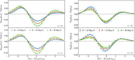
Simulated (data points) and predicted (lines) differences from ΛCDM of the modified gravity matter PDF at z = 0 (top) and z = 1 (bottom). The density field is averaged in spheres of radius R = 10 |$\mathrm{Mpc}\, h^{-1}$| (blue), 15 |$\mathrm{Mpc}\, h^{-1}$| (orange), and 20 |$\mathrm{Mpc}\, h^{-1}$| (green). Solid lines are obtained from the measured non-linear variance, |$\sigma ^2_\mu$|, while dashed lines use equation (21) in pyLDT. The close agreement between the two type of predictions supports the use of the lognormal approximation for the non-linear variance. Left: in DGP the shape of these changes is very similar to that induced by variations in σ8 (cf. fig. 8 in Uhlemann et al. 2020). Right: f(R) gravity departures from the standard cosmology are more prominent for underdense regions and become less significant with increasing smoothing radii owing to the finite range of the fifth force.
4.1.1 Pseudo-cosmologies
Although, by definition, for the pseudo cosmologies we have |$\sigma _{\rm L}^{\rm pseudo}(R,z_{\rm f}) = \sigma _{\rm L}^{\rm real}(R,z_{\rm f})$| (see equation 22), new late-time physics affects the growth of structure beyond the linear regime. Therefore, the non-linear power spectrum of the pseudo-cosmology differs from its real non-ΛCDM counterpart and |$\sigma _{\rm NL}^{\rm pseudo}(R,z_{\rm f}) \ne \sigma _{\rm NL}^{\rm real}(R,z_{\rm f})$|. We can use this to compute the PDFs of the pseudo-MG cosmologies and compare them to the predictions for DGP and f(R) gravity – given the identity in equation (22), any significant difference not captured by a simple change to the non-linear variance will then signal modifications to the spherical dynamics due to the action of the fifth force. We recall that the linear power spectrum determines the scale dependence of the linear variance and hence the density dependence of the exponent of the PDF given by equation (4), while the non-linear power spectrum determines the non-linear variance and hence the width of the PDF. To a lesser extent, the non-linear variance can also alter the scale dependence of the PDF through its impact on the rescaling step in the PDF construction (see equation 5c).
Fig. 6 shows the difference between the real and pseudo-cosmology PDFs for DGPm (left-hand panel) and F5 (right-hand panel). First, let us note that these differences are about an order of magnitude smaller than the departures of modified gravity from ΛCDM shown in Fig. 5. In general, the two PDFs agree to per cent level or better for |ln ρ − 〈ln ρ〉| < 2σln ρ. Thus, for densities not too far into the tails and in the mildly non-linear regime, the pseudo and real cosmology PDFs become indistinguishable for all intents and purposes. This result confirms the findings of Cataneo et al. (2019) and extends them to statistics describing non-Gaussian properties of the density field. Our predictions using the EdS spherical collapse for both the pseudo and the real MG cosmologies (solid lines) can partially explain the observed minute differences as changes in the variance of the distribution, especially at high redshifts. To gauge the contribution of the fifth force to the remaining unexplained difference, we also compute the PDFs for DGPm by including the linearized modification to the gravitational interaction (equation 11) into the dynamics of spherical top-hat density fluctuations (equation 8). These are shown as dashed lines in Fig. 6. Although the modified non-linear evolution can better account for the differences between the real and pseudo-cosmology, residuals associated with the neglected screening mechanism and intrinsic inaccuracies of the LDT formalism persist. To fully disentangle these two contributions one should run linearized modified gravity simulations (akin to Schmidt 2009; Koyama et al. 2009), which is, however, beyond the scope of this work. For the case of f(R) gravity shown in the right-hand panel, a change in the variance (solid line) can only partially explain their observed differences. Modifications to the spherical collapse in f(R) gravity due to non-linear couplings even in the absence of screening (such as modelled by Brax & Valageas 2012) are a potential source of the remaining discrepancy. The shape of the differences hints at an additional skewness with a slightly increased S3 that cannot be captured by the EdS-based approximation in equation (9). The overall good agreement of the PDF in the real and pseudo-cosmologies together with the successful prediction of their minute qualitative differences validate our PDF modelling assumptions for modified gravity.
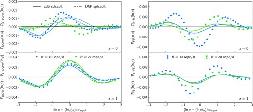
Simulated (data points) and predicted (lines) differences of the modified gravity matter PDFs from their pseudo-cosmology counterparts at z = 0 (top) and z = 1 (bottom). The density field is averaged in spheres of radius R = 10 |$\mathrm{Mpc}\, h^{-1}$| (blue) and 20 |$\mathrm{Mpc}\, h^{-1}$| (green). Solid lines are obtained from the measured non-linear variance, |$\sigma ^2_\mu$|, and the EdS mapping shown in Fig. 1. Note that the amplitude of these differences is about ten times smaller than in Fig. 5, confirming the remarkable similarities between the pseudo and real cosmology on mildly non-linear scales. Left: by replacing the EdS spherical evolution with that produced by the linearized DGP model (dashed lines) we can better predict some of the minute differences sourced by pure modifications to GR which are not captured by simple changes to σ8 in a ΛCDM cosmology. Remaining differences are likely the result of modelling inaccuracies in LDT and unaccounted for Vainshtein screening phenomenology. Right: contrary to DGP, the violation of Birkhoff’s theorem in f(R) gravity precludes any attempt to find a simple solution to the evolution of spherical top-hat density perturbations even in the absence of screening mechanism (Borisov et al. 2012; Brax & Valageas 2012; Kopp et al. 2013). Here we only show the predictions accounting for changes in the non-linear variance and note that both the finite range of the fifth force and chameleon screening slightly modify the spherical collapse dynamics, which in turn leads to small additional variations in the PDF.
4.2 Evolving dark energy
Analogously to modified gravity, the fractional deviations of the theory predictions from the simulation measurements shown in Fig. 7 confirm that, despite neglecting the impact of dark energy on the spherical collapse, the LDT prescription in equation (19) yields accuracies within a few per cent for densities |ln ρ − 〈ln ρ〉| < 2σln ρ. Although the results presented here are only for density fields averaged in spheres of radius R = 10 |$\mathrm{Mpc}\, h^{-1}$|, we found similar or better performance for larger smoothing radii. Fig. 8 illustrates that in most cases deviations from the cosmological constant can be described very well by simple changes to the non-linear variance (lines). In fact, after fixing the standard cosmological parameters, the w0waCDM and ΛCDM cosmologies share the same shape of the linear matter power spectrum, and when using the EdS approximation for the spherical dynamics the only degree of freedom left in equation (4) is the non-linear variance. However, the small yet visible discrepancies between theory and simulations for the w0 = −0.5 cosmology suggest that in this extreme scenario the background expansion appreciably alters the spherical evolution and it should be taken into account to accurately predict the measured PDF deviations from ΛCDM at both redshifts.
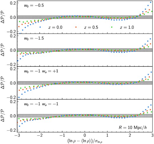
Residuals between the measured and predicted matter PDF in spheres of radius 10 |$\mathrm{Mpc}\, h^{-1}$| normalized to the theory predictions for various evolving dark energy cosmologies (from top to bottom). Different colours correspond to z = 0 (blue), z = 0.5 (orange), and z = 1 (green). The solid and dashed lines mark the 1 and 2 per cent accuracy, respectively. Note that for these simulations only one realization is available, and the estimation of the smoothed density field differs from that used for the modified gravity simulations. Despite these differences the residuals are consistent with those for ΛCDM, f(R) gravity, and DGP in Fig. 4.
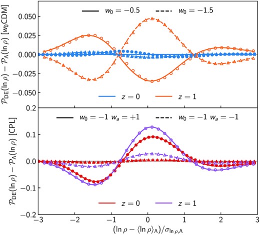
Measured (data points) and predicted (lines) differences from ΛCDM of the w0CDM (top) and the w0waCDM (bottom) cosmologies at z = 0 and z = 1. The density field is averaged in spheres of radius R = 10 |$\mathrm{Mpc}\, h^{-1}$| and the linear power spectra for all cosmologies (except {w0, wa} = {−1, +1}) are normalized such that |$\sigma _8^{\rm DE}(z=0) = \sigma _8^{\Lambda }(z=0)$|. Predictions are obtained from the measured non-linear variance, |$\sigma ^2_\mu$|, together with EdS spherical collapse. Except for w0 = −0.5, knowledge of the non-linear variance is enough to accurately describe departures from the standard cosmology.
4.3 Fisher forecasts
This section presents forecasts for DGP and f(R) gravity and w0waCDM combining the matter PDF and the matter power spectrum on mildly non-linear scales. For the MG models we determine the ability of future experiments to detect relatively small deviations from GR (i.e. F6 and DGPw) at a statistical significance >5σ (see Table 2), while for evolving DE we will be interested in the FoM using ΛCDM as fiducial cosmology (see Table 3).
4.3.1 Fisher formalism
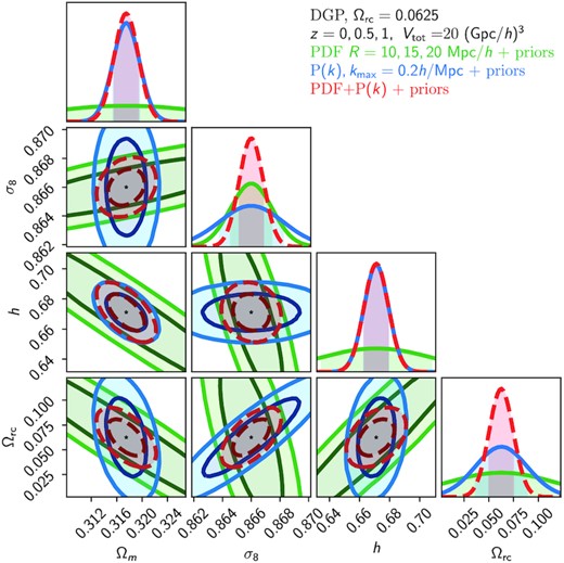
Marginalized Fisher forecast constraints on {Ωm, σ8, h, Ωrc} using external prior information on ns and Ωb (as described in the text) for a DGPw fiducial cosmology. Contours correspond to the matter PDF at 3 scales and 3 redshifts (green), the matter power spectrum up to k = 0.2 h Mpc−1 (blue), and their combination, which includes the covariance between the PDF and power spectrum (red dashed).
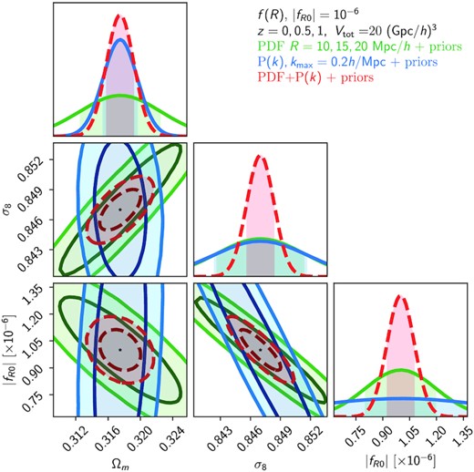
Marginalized Fisher forecast constraints on {Ωm, σ8, |fR0|} using external prior information on ns and Ωb (as described in the text) for an F6 fiducial cosmology. Contours correspond to the matter PDF at 3 scales and 3 redshifts (green), the matter power spectrum up to k = 0.2 h Mpc−1 (blue), and their combination, which includes the covariance between the PDF and the power spectrum (red dashed).
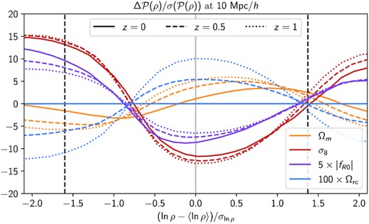
Comparison of PDF differences divided by the error on the PDF as estimated from the quijote simulations. Line style indicates the redshift, while colour indicates parameter being deviated. The vertical lines represent the region used at each redshift to construct the PDF data vector. While the shape of the σ8 and Ωrc derivatives are similar, their different redshift dependence allows the degeneracy to be broken when combining redshifts. The fR0 derivatives, in addition to having different redshift dependence, exhibit a skewness not present in the σ8 derivatives, allowing significant information to be extracted even at a single redshift, including z = 0. Note that the amplitudes between parameters should not be directly compared, as the fR0 and Ωrc lines have been scaled up to be visible on the same scale as σ8.
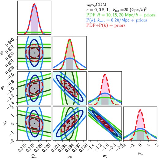
Fisher forecast constraints on {Ωm, σ8, w0, wa} (marginalized over {Ωb, ns} using the external prior described in the text) for the w0CDM model around the fiducial quijote ΛCDM cosmology. Contours correspond to the matter PDF at 3 scales and 3 redshifts (green), the matter power spectrum up to k = 0.2 h Mpc−1 (blue), and their combination which includes the covariance between the PDF and power spectrum (red dashed).
In this work, we use the covariance matrix obtained from a set of 15 000 simulations of the quijote N-body simulation suite (Villaescusa-Navarro et al. 2020) using the fiducial ΛCDM cosmology (Ωm = 0.3175, Ωb = 0.049, H0 = 68 km s−1 Mpc−1, ns = 0.96, σ8 = 0.834). The joint covariance matrix of the mildly non-linear matter PDF and the matter power spectrum is described in Uhlemann et al. (2020), see particularly their fig. 12. We make the approximation that the covariance matrix of the matter PDF and matter power spectrum in the mildly non-linear regime is independent of cosmology and theory of gravity and well-captured by the 15 000 simulations of the quijote simulation suite. To mitigate potential effects of modified gravity on the covariance, we fix the standard cosmological parameters to the values of the fiducial quijote cosmology. In particular, we set As = 2.13 × 10⁻⁹ such that σ8 increases only slightly for the modified gravity cosmologies, that is, by 1.6 per cent for F6 and 3.8 per cent for DGPw. As those are small perturbations from the fiducial ΛCDM cosmology, they will only induce a small error on the true covariances and hence only marginally affect parameter constraints. As this error will affect both the PDF and power spectrum covariance in a similar way, comparisons of their respective constraining power are expected to be robust. For future high precision cosmology, covariance estimation for PDF-based observables from galaxy clustering and weak lensing can rely on tuned lognormal mocks (Gruen et al. 2018; Boyle et al. 2021), potentially complemented with predictions for effects induced by variations in the local mean density (Jamieson & Loverde 2020). To correct for a potential bias depending on the size of the data vector NS compared to the number of simulations Nsim, we multiply the inverse of the simulated covariance matrix by the Kaufman–Hartlap factor (Kaufman 1967; Hartlap, Simon & Schneider 2006), fKH = (Nsim − 2 − NS)/(Nsim − 1). Since in our case the number of simulations for covariance estimation is very large (15 000) compared to the maximal length of the data vector (218 for our three-redshift analysis of the PDF at three scales and the mildly non-linear power spectrum), this factor will be close to one throughout, fKH ≥ 0.985. We mimic a Euclid-like effective comoving survey volume of |$V \approx 20 \, ({\rm Gpc}\,h^{ -1})^3$| split across three redshift bins of equal width Δz = 0.2 located at z = 0, 0.5, 1 by multiplying the covariance at each redshift with the ratio of the comoving shell volume to the simulation volume |$V_{\rm sim}=1 \, ({\rm Gpc}\,h^{ -1})^3$|.
4.3.2 Modified gravity
We now compare the constraining power of the matter PDF to that of the matter power spectrum (with |$k_{\rm max} = 0.2 \ h \ \rm Mpc^{-1}$|) for DGP and f(R) gravity. In all cases, the forecasts shown are marginalized over all remaining ΛCDM parameters.
Figs 9 and 10 show the Fisher forecasts for DGP and f(R) cosmologies, respectively. Table 2 summarizes the detection significance for particular flavours of these modified gravity models expressed in units of standard deviation from GR. In a universe where the growth of structure is governed by DGP gravity with Ωrc = 0.0625, a 5σ detection of modified gravity can still be reached by combining the matter PDF with the matter power spectrum. Combining the PDF and power spectrum as complementary probes is beneficial in both MG scenarios. In particular, for DGP the matter PDF is important for constraining σ8, while the power spectrum is important for obtaining the correct value of Ωm. This is because while Ωm has a distinctive signature in the power spectrum (see Fig. C3), the matter PDF is sensitive to the total matter density only through its impact on the skewness and the linear growth factor, D(z). The anticorrelation between the Hubble parameter, h, and Ωm visible in Fig. 9 can be explained by their similar impact on the skewness of the PDF (see fig. 9 in Uhlemann et al. 2020). Evolving dark energy also presents this feature, although we do not show it in Fig. 12 as it does not create any unexpected degeneracy directions as in the DGP model.
The partial degeneracy in the PDF between σ8 and the modified gravity parameters, |fR0| or Ωrc, seen in Figs 9 and 10 is understood by noticing that the presence of modified gravity changes the width of the matter PDF, as can be seen in Fig. 11. However, the responses of the PDF to the presence of modified gravity or changes in σ8 have different scale and time dependence, therefore by combining the information from different scales and redshifts we can break this degeneracy. Fig. 11 shows that σ8 and Ωrc have opposite effects on the PDF, which would lead to a positive correlation between these parameters. However, in Fig. 9 the σ8–Ωrc plane shows an anticorrelation for the PDF, which is indirectly induced by the strong positive correlation between Ωrc and h. We checked that when h is fixed to its fiducial value, rather than marginalized over, the PDF contours do indeed display a positive correlation between σ8 and Ωrc, as indicated by the derivatives in Fig. 11.
In the case of f(R) gravity, the matter PDF is particularly useful, reaching a 5σ detection before combining with the matter power spectrum. This is due to an additional skewness in the |fR0| derivatives sourced by the scale-dependent fifth force and the fact that the PDF holds information about deviations from ΛCDM even at redshift 0, unlike in DGP. However, Fig. C2 shows that using the non-linear variance predicted by equation (21) is a better approximation in DGP than in f(R) gravity, and we thus expect the forecasted constraints to be more reliable for the DGP model than for f(R) gravity.
4.3.3 Evolving dark energy
Increasing either w0 or wa increases the growth rate and hence the variances at z > 0 (with marginal changes at z = 0 due to fixed σ8), which amounts to an anticorrelation between w0 and wa. Most of the other degeneracy directions in the w0waCDM case can be understood by considerations of linear theory. Changing a single parameter at fixed σ8 (or similarly when σ8 is allowed to vary) induces a change in the growth rate. Suitable pairs of parameters can then produce growth rates close to the fiducial cosmology. For example, the positive correlation between w0 and Ωm arises from the suppression of the growth rate by increasing Ωm while keeping σ8 fixed. While one would expect w0 and wa to vary in the same way with Ωm and σ8, they in fact vary in opposing directions as shown in Fig. 12. However, when w0 is fixed to its fiducial value, rather than marginalized over, the contours do indeed flip in sign to the direction expected, suggesting that the tight anticorrelation in the w0–wa plane dominates the other degeneracies.
5 SUMMARY AND DISCUSSION
To harness the full statistical power of current and forthcoming galaxy surveys we must push past 2-point correlation functions. Gravitationally driven non-Gaussianities are particularly sensitive to the late-time growth of structure. As a result, the full shape of the matter density PDF responds strongly to departures from GR and the cosmological constant making it a promising probe of new physics. In this work we built on the findings of Uhlemann et al. (2016) with the aim of extending the large-deviation theory formalism for the 3D matter PDF to cosmologies with universally coupled fifth forces and non-standard expansion histories. As for ΛCDM, our analytical predictions are derived from linear theory calculations and spherical collapse dynamics, with the fiducial non-linear variance being a free parameter that can be measured from simulations. However, contrary to previous approaches (cf. Brax & Valageas 2012), we approximate the collapse or expansion of spherical top-hat fluctuations with a EdS evolution, and showed that in the mildly non-linear regime this choice produces PDFs matching the simulations to better than a few per cent around the peak of the distribution. Although in this work we analysed in great detail specific modified gravity and dark energy cosmologies, our method is readily applicable to more general models, as changes to the standard cosmology only enter the PDF through the linear matter power spectrum and the non-linear variance of the smoothed density field. We also implemented the LDT equations in pyLDT, an easy-to-install and user-friendly python package that enables fast calculations of the PDF of the spherically averaged matter density field in ΛCDM, modified gravity and evolving dark energy cosmologies. We employed pyLDT in Fisher analyses of a Euclid-like survey to estimate the additional information brought in by the matter PDF compared to 2-point statistics restricted to mildly non-linear scales. In all cases investigated the constraints on new physics (be it Geff ≠ GNewton or w ≠ −1) from the combination of the matter PDF and power spectrum are substantially tighter than those obtained separately by the two statistics – a clear sign of complementarity (see also Uhlemann et al. 2020, for massive neutrino cosmologies). For modified gravity, adding the matter PDF to the power spectrum can double the detection significance for the DGPw model to lift it above 5σ and increase the F6 detection significance sixfold as summarized in Table 2. For dark energy, combining the matter PDF with the power spectrum can also double our constraining power on the clustering amplitude, σ8, and both of the dark energy equation of state parameters w0 and wa as shown in Table 3.
In spite of the idealized experimental set-up focusing on the statistics of the 3D matter field, our results are also encouraging for more realistic scenarios. The formalism described in this paper can be translated to galaxy survey observables accessible from weak lensing (Barthelemy et al. 2020; Boyle et al. 2021; Thiele, Hill & Smith 2020), galaxy clustering (Repp & Szapudi 2020; Friedrich et al. 2022) as well as their combination in density-split statistics (Friedrich et al. 2018; Gruen et al. 2018), which have been shown to be able to simultaneously extract galaxy bias, galaxy stochasticity, and cosmological parameters. In particular, the LDT approach developed for the ΛCDM lensing convergence PDF could be straightforwardly applied to the entire class of scalar–tensor theories with lensing potential |$\Phi _{\rm lens}^{\rm MG} \approx \Phi _{\rm lens}^{\rm GR}$|, which includes f(R) gravity and DGP. The PDF could also be useful for disentangling modified gravity and massive neutrinos (Giocoli, Baldi & Moscardini 2018), but we leave the combination of those two scenarios for future work. Including the PDF of observable fields like cosmic shear or galaxy counts could help break degeneracies between astrophysical (e.g. baryonic feedback, intrinsic alignment, and galaxy bias) and cosmological parameters present in the analyses of two-point statistics (Patton et al. 2017; Hadzhiyska et al. 2021).
ACKNOWLEDGEMENTS
We are grateful to Marius Cautun for his support in setting up dtfe, to Fabian Schmidt for sharing his 1D relaxation code at an early stage of this work, to Alexandre Barreira for giving access to his DGP simulations, to Jihye Shin for sharing the means and variances of the DE simulations, and to Alexander Mead for his support with hmcode. We also thank Yanchuan Cai and Wojciech Hellwing for useful discussions. The figures in this work were created with matplotlib (Hunter 2007) and chaincosumer (Hinton 2016), making use of the numpy (Harris et al. 2020) and scipy (Virtanen et al. 2020) Python libraries. MC and CH acknowledge support from the European Research Council under grant number 647112. CH also acknowledges support from the Max Planck Society and the Alexander von Humboldt Foundation in the framework of the Max Planck-Humboldt Research Award endowed by the Federal Ministry of Education and Research. AG is supported by an EPSRC studentship under Project 2441314 from UK Research & Innovation. CA and BL are supported by the European Research Council (ERC) through a starting Grant (ERC-StG-716532 PUNCA). BL is further supported by the UK Science and Technology Funding Council (STFC) Consolidated Grant No. ST/I00162X/1 and ST/P000541/1. This work used the DiRAC@Durham facility managed by the Institute for Computational Cosmology on behalf of the STFC DiRAC HPC Facility (www.dirac.ac.uk). The equipment was funded by BEIS capital funding via STFC capital grants ST/K00042X/1, ST/P002293/1, ST/R002371/1, andST/S002502/1, Durham University and STFC operations grant ST/R000832/1. DiRAC is part of the National e-Infrastructure.
DATA AVAILABILITY
Our code to compute the matter PDF predictions is publicly available at https://github.com/mcataneo/pyLDT-cosmo. The f(R) gravity simulation data used in this paper may be available upon request to the corresponding author. The matter PDF measured from the Quijote simulations are publicly available at https://quijote-simulations.readthedocs.io/en/latest/. The matter PDF measurements for the dark energy cosmologies are publicly available at https://astro.kias.re.kr/jhshin/.
Footnotes
Physically speaking, this procedure amounts to asserting that the reduced cumulants (discussed later), encoded in the large deviation statistics rate function and predicted from spherical collapse in the limit σ2 → 0, can reliably be extrapolated to small, non-zero variances (as demonstrated with simulated data in Uhlemann et al. 2016). The |$\sigma _{\rm NL}^2$| factor in the denominator then plays the role of converting the reduced cumulants back to the cumulants using the correct non-linear variance, which controls the width of the PDF.
At first glance this result seems at odds with the notion that dark energy and modified gravity affect the growth of structure. However, here we are fixing the final non-linear density, ρ, such that enhancements (suppressions) of the linear growth require lower (higher) initial density contrasts, δini, to match that particular ρ. In other words, adjustments to the initial conditions compensate for the linear growth modifications to a very good approximation.
Technically speaking, DGP is a higher dimensional theory of gravity that falls outside the Horndeski theory landscape. However, the scales relevant for structure formation are well within the regime in which DGP can be treated as a 4D scalar–tensor theory (Nicolis & Rattazzi 2004; Park, Zurek & Watson 2010).
Here, R denotes the Ricci scalar and it must not be confused with the smoothing radius defined above. In what follows we shall keep the same notation for both quantities as their meaning should be clear from context.
Note that the common approximation for the linear growth |$D(z)\propto H(a)\int _0^a {\rm d} a^{\prime } (a^{\prime } H(a^{\prime }))^{-3}$| [quoted in equation (6) of Codis et al. (2016) and (A1) of Uhlemann et al. (2020)] is not accurate enough to estimate the response of the PDF to changing w beyond a cosmological constant.
Because the linear theory normalization cancels out in equation (4), knowledge of σ8 is irrelevant for the LDT predictions when measurements of the variance of the simulated density field are available. In fact, the non-linear variance carries information on σ8 so that, ultimately, its impact on the theory PDF is properly accounted for.
REFERENCES
APPENDIX A: THE IMPACT OF MASS-ASSIGNMENT SCHEMES ON THE PDF
The various methods designed to interpolate the simulated density field on a grid may lead to differences between the measured PDFs large enough to potentially bias the predictive accuracy of a particular theoretical framework. In Fig. A1, we compare two such popular methods–the CiC algorithm and the Delaunay tassellation field estimator – using as summary statistic the PDF extracted from a single snapshot after applying top-hat filters with three different smoothing radii. Reassuringly, the distributions agree to better than 1 per cent for all densities but the rarest underdensities, thus validating the performance of LDT discussed in Section 4 and previously presented in Uhlemann et al. (2020).
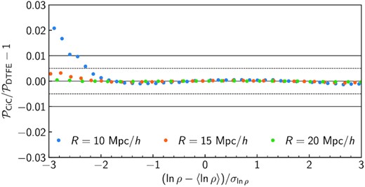
Relative deviation between the matter PDF constructed from the CiC mass-assignment scheme and that based on the Delaunay tassellation (DTFE). Data points represent measurements from a single z = 0 snapshot of a ΛCDM simulation. The agreement between the two mass-assignment schemes is excellent over the entire range of densities relevant for this work.
APPENDIX B: MEANS AND VARIANCES OF THE SIMULATED NON-LINEAR DENSITY FIELD
Table B1 lists variances and means extracted from the simulations for various smoothing radii and redshifts, which we used to produce the ΛCDM and modified gravity results presented in Section 4. The corresponding quantities for the dark energy cosmologies can be requested to the authors of Shin et al. (2017).
Measured variances and means of the smoothed density and log-density field for the standard cosmology, f(R) gravity with |fR0| = 10−5 and DGP gravity with Ωrc = 0.25. All values for ΛCDM and F5 are the average over eight realizations.
| . | ΛCDM . | F5 . | DGPm . | ||||||
|---|---|---|---|---|---|---|---|---|---|
| . | |$\sigma _\rho ^2$| . | |$\sigma _\mu ^2$| . | 〈μ〉 . | |$\sigma _\rho ^2$| . | |$\sigma _\mu ^2$| . | 〈μ〉 . | |$\sigma _\rho ^2$| . | |$\sigma _\mu ^2$| . | 〈μ〉 . |
| R = 10 Mpc h−1 | |||||||||
| z = 0 | 0.567 | 0.392 | −0.205 | 0.612 | 0.428 | −0.223 | 0.716 | 0.465 | −0.246 |
| z = 1 | 0.195 | 0.167 | −0.0836 | 0.199 | 0.171 | −0.0857 | 0.223 | 0.188 | −0.0953 |
| R = 15 Mpc h−1 | |||||||||
| z = 0 | 0.276 | 0.233 | −0.118 | 0.291 | 0.248 | −0.126 | 0.345 | 0.282 | −0.144 |
| z = 1 | 0.0993 | 0.093 | −0.0468 | 0.101 | 0.0945 | −0.0475 | 0.114 | 0.106 | −0.0532 |
| R = 20 Mpc h−1 | |||||||||
| z = 0 | 0.163 | 0.149 | −0.0745 | 0.17 | 0.157 | −0.078 | 0.204 | 0.184 | −0.0922 |
| z = 1 | 0.0598 | 0.0579 | −0.0285 | 0.0603 | 0.0586 | −0.0288 | 0.0684 | 0.0661 | −0.033 |
APPENDIX C: VALIDATION OF LDT PREDICTIONS FOR SMALL DEVIATIONS FROM ΛCDM FIDUCIAL
C1 Modified gravity
Our theoretical prediction for the matter PDF have been validated with numerical simulations in the main text for the two modified gravity models F5 and DGPm (see Fig. 5). Figs C1 and C2 illustrate the accuracy of the theoretical predictions for F6 and DGPw in the form of residuals from the simulations and departures from ΛCDM, as well as the impact of using the lognormal approximation (equation 21) in pyLDT.
C2 Dark energy
Our theoretical prediction for the matter PDF have been validated with numerical simulations in the main text for large changes in the parametrized dark energy equation of state (see Fig. 8). A similar comparison for all ΛCDM parameters has been provided in Uhlemann et al. (2020), see figs 8 and 9 therein. Here, we provide complementary results for the full set of w0CDM parameters available from the Quijote simulations (Villaescusa-Navarro et al. 2020).
To further validate our joint matter PDF and matter power spectrum constraints, we compare theoretical power spectrum derivatives from hmcode to measured derivatives from the Quijote simulations in Fig. C3. When limiting ourselves to mildly non-linear scales |$k\lt k_{\rm max}=0.2 \ h\, \mathrm{Mpc}^{-1}$| we find good agreement between the two. We notice slight discrepancies for some parameters that turn out to be unimportant when constraining just a few parameters, but hampering agreement between theory and simulation matter power spectrum in a Fisher forecast simultaneously varying all w0CDM parameters. To mitigate this minor issue for the power spectrum, we decided to include an external prior on {Ωb, ns}, as described in the main text.
Using this prior, we successfully validated the constraints obtained using our theoretical derivatives against simulations by performing a Fisher forecast with all six w0CDM parameters for which derivatives are available from the Quijote simulation suite. In Fig. C4, we demonstrate that we obtain virtually identical results for both the degeneracy directions and the individual parameter constraints when marginalized over all other parameters.
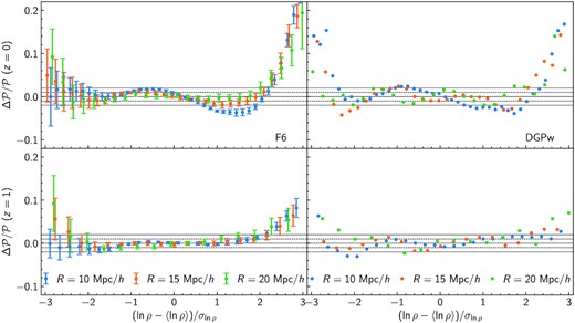
Residuals between the measured and predicted matter PDF normalized to the theory predictions for z = 0 (top) and z = 1 (bottom) in f(R) gravity with |fR0| = 10−6 (left) and DGP with Ωrc = 0.0625 (right). Different colours indicate the radii of the spheres used for smoothing the density field, 10 (blue), 15 (orange), and 20 |$\mathrm{Mpc}\, h^{-1}$| (green). The solid and dashed lines mark the 1 and 2 per cent accuracy, respectively.
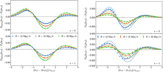
Measured (data points) and predicted (lines) responses of the matter PDF to modified gravity at z = 0 (top) and z = 1 (bottom). The density field is averaged in spheres of radius R = 10 (blue), 15 (orange), and 20 |$\mathrm{Mpc}\, h^{-1}$| (green). Solid lines are obtained from the measured non-linear variance, |$\sigma ^2_\mu$|, while dashed lines from its approximation equation (21) used in pyLDT. Left: differences from ΛCDM for DGP gravity with Ωrc = 0.0625. Right: same as left-hand panel for f(R) gravity with |fR0| = 10−6.
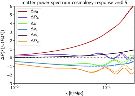
Validation of matter power spectrum derivatives up to kmax = 0.2 |$h\, \mathrm{Mpc}^{-1}$| at z = 0.5 as obtained from hmcode (dashed lines) compared to measurements in the Quijote simulation suite (solid lines) for the full set of 6 cosmological parameters for w0CDM. We show the results as a signal-to-noise like ratio of the differences in the matter power spectrum, ΔP(k), and the expected error on the fiducial power spectrum from the diagonal of the covariance matrix, σ(P0(k)).
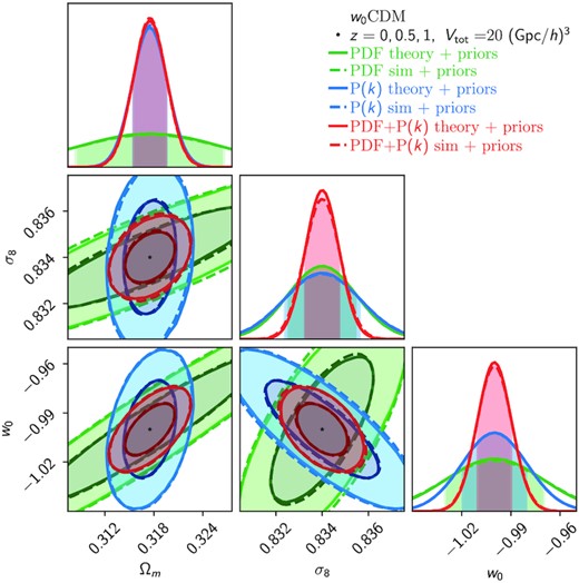
Marginalized constraints on Ωm, σ8, and w0 from a w0CDM Fisher forecast obtained from using the theory derivatives for the matter PDF and power spectrum (solid lines) or the simulated derivatives from the Quijote simulation suite (dashed lines), both when including a prior on {Ωb, ns}. This validates the robustness of our theoretical predictions used for the forecasts in the main text.


