Centrifugal breakout reconnection as the electron acceleration mechanism powering the radio magnetospheres of early-type stars Free

ABSTRACT

1 INTRODUCTION

Hot luminous, massive stars of spectral types O and B have dense, high-speed, radiatively driven stellar winds (Castor, Abbott & Klein 1975). In the subset (∼10 per cent; Grunhut et al. 2017; Sikora et al. 2019a) of massive stars with strong (⁠|$\gt \, 100$| G; Aurière et al. 2007; Shultz et al. 2019a), globally ordered (often significantly dipolar; Kochukhov, Shultz & Neiner 2019) magnetic fields, the trapping of this wind outflow by closed magnetic loops leads to the formation of a circumstellar magnetosphere (Petit et al. 2013). Because of the angular momentum loss associated with their relatively strong, magnetized wind (ud-Doula, Owocki & Townsend 2009), magnetic O-type stars are typically slow rotators, with trapped wind material falling back on a dynamical time-scale, giving what is known as a dynamical magnetosphere (DM).

But in magnetic B-type stars, the relatively weak stellar winds imply longer spin-down times, and so a significant fraction that still retains a moderately rapid rotation; for cases in which the associated Keplerian co-rotation radius R_K lies within the Alfvén radius R_A that characterizes the maximum height of closed loops, the rotational support leads to formation of a centrifugal magnetosphere (CM), wherein the much longer confinement time allows material to build up to a sufficiently high density to give rise to distinct emission in H α and other hydrogen lines (Landstreet & Borra 1978). A recent combination of empirical (Shultz et al. 2020) and theoretical (Owocki et al. 2020) analyses showed that both the onset and strength of such Balmer α emission is well explained by a centrifugal breakout (CBO) model, wherein the density distribution of material within the CM is regulated to be near the critical level that can be contained by magnetic tension (ud-Doula, Owocki & Townsend 2008). The upshot is that such hydrogen emission arises only in magnetic stars with both strong magnetic confinement and moderately rapid stellar rotation.

Another distinctive observational characteristic of many such magnetic B-stars is their non-thermal, circularly polarized radio emission, thought to arise from gyrosynchrotron emission by energetic electrons trapped within closed magnetic loops. An initially favoured model by Trigilio et al. (2004) proposed that these electrons could be accelerated in the current sheet (CS) between field lines of opposite polarity that have been stretched outward by the stellar wind, as illustrated in the left-hand panel of Fig. 1. But a recent empirical analysis by Leto et al. (2021) has shown that the observed radio emission has a clear dependence on stellar rotation, providing strong evidence against this CS model, which includes no role for rotation. Instead, Leto et al. (2021) noted that their fits to the radio luminosity scale in proportion to a quantity that has the physical dimension of an electromotive force (EMF), which they speculated may be suggestive of an underlying mechanism. Indeed, the EMF is invoked (Hill 2001) to model auroral emission from the interaction of high-energy magnetospheric particles with planetary atmospheres. However, such thermal atmospheric auroral dissipation of EMF-accelerated particles in the magnetosphere cannot explain the polarized radio emission that likely arises from gyrosynchrotron processes in the highly conductive magnetosphere itself.

Figure 1.

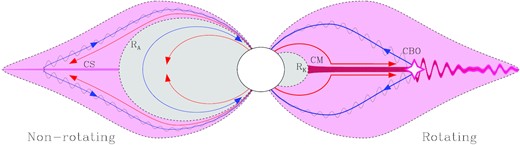
Schematic to contrast the previous Trigilio et al. (2004) CS model for electron acceleration and radio emission (left) with our proposed CBO model for electron acceleration from CBO-driven magnetic reconnection events (right). Pink-shaded regions indicate magnetic field lines contributing plasma to the electron acceleration, while grey shading indicates regions isolated from the locus of electron acceleration. A key distinction regards the lack of a dynamical role for rotation in the CS model, in contrast to the inferred empirical dependence on rotation, which is well matched in the CBO model. Figure adopted from fig. 8 of Paper I, which contains further details on the schematic.

Open in new tabDownload slide

The alternative theoretical scalings explored here were motivated by a more recent companion empirical analysis by Shultz et al. (2022, hereafter Paper I), which confirms the basic results of Leto et al. (2021), but within a significantly extended sample that allows further exploration of potential empirical trends and scalings. In particular, we show below (Section 3) that these empirical scalings for non-thermal radio emission can be well fitted by models grounded in the same CBO paradigm that has been so successful for H α emission. Specifically, it is now the magnetic reconnection associated with CBO events that provides the non-thermal acceleration of electrons, which then follow the standard picture of gyrosynchrotron emission of observed circularly polarized radio.

Fig. 1 graphically illustrates the key distinctions between this new CBO paradigm (right) from the previous CS-acceleration model (left) proposed by Trigilio et al. (2004).

To lay the groundwork for derivation in Section 3 of these scalings for radio emission from CBO-driven reconnection, Section 2 reviews the basic CM model and the previous application of the CBO paradigm to H α. In Section 4, we contrast our results with the EMF-based picture, and discuss the potential further application of the CBO paradigm, including for modelling the stronger X-ray emission of CM versus DM stars (Nazé et al. 2014). We conclude (Section 5) with a brief summary and outlook for future work.

2 BACKGROUND

2.1 Dynamical versus centrifugal magnetospheres

In contrast, for stars with both moderately rapid rotation (W ≲ 1) and strong confinement (η_* ≫ 1), one finds R_K < R_A. In the region R_K < r < R_A, magnetic tension still confines material while the centrifugal force prevents gravitational fallback, thus allowing material build-up into a much denser CM.

2.2 Centrifugal breakout and H α emission

Motivated by this key result, Owocki et al. (2020) examined the theoretical implications of this CBO-limited density scaling for such H α emission, showing that it can simultaneously explain the onset of emission, the increase of emission strength with increasing magnetic field strength and decreasing rotation period, and the morphology of emission line profiles (Owocki et al. 2020; Shultz et al. 2020). As initially suggested by Townsend & Owocki (2005), the breakout density at R_K is set by B_K, and is independent of |$\dot{M}$|⁠; precisely this dependence on B_K, and lack of sensitivity to |$\dot{M}$|⁠, was found by Shultz et al. (2020) for both emission onset and emission strength scaling. Owocki et al. (2020) found an expression for the strength B_K1 necessary for the density at R_K to produce an optical depth of unity in the H α line, and showed that the threshold B_K/B_K1 neatly divides stars with and without H α emission. Two-dimensional MHD simulations of CBO by ud-Doula, Townsend & Owocki (2006) and ud-Doula et al. (2008) yielded a radial density gradient associated with the CBO mechanism, which in conjunction with the density at R_K set by B_K can be used to predict the optically thick area and, hence, the scaling of emission strength (Owocki et al. 2020). Finally, a characteristic emission line profile morphology, common across all H α-bright CM host stars, was reported by Shultz et al. (2020) and shown by Owocki et al. (2020) to be a straightforward consequence of a co-rotating optically thick inner disc transitioning to optically translucent in the outermost region.

A crucial subtlety that deserves emphasis is that, in contrast to expectations from 2D MHD simulations that CBO should manifest as catastrophic ejection events accompanied by large-scale reorganization of the magnetosphere (ud-Doula et al. 2006, 2008), which has indeed never been observed in the densest inner regions (Townsend et al. 2013; Shultz et al. 2020), the H α analysis performed by Shultz et al. (2020) instead indicates that the magnetosphere must be continuously maintained at breakout density, with CBO occurring more or less continuously on small spatial scales. However, it is worth noting that the ‘giant electron-cyclotron maser (ECM) pulse’ observed by Das & Chandra (2021) may have been the signature of a large-scale breakout occurring in magnetospheric regions in which the density is too low to be probed by H α or photometry.

H α emission and gyrosynchrotron emission occur in the same part of the rotation-magnetic confinement diagram (see fig. 3 in Paper I), and H α emission EW and radio luminosity are closely correlated (see fig. 6 in Paper I). Since H α emission is regulated by CBO, this suggests that the same may be true of gyrosynchrotron emission. In the following, we develop a theoretical basis for this connection, which we then compare to the empirical regression analyses and measured radio luminosities.

3 CBO-DRIVEN MAGNETIC RECONNECTION

3.1 Rotational spin-down

The Weber & Davis (1967) analysis treated the simple case of a pure radial field from a spilt monopole, with p = 1. But ud-Doula et al. (2008) showed a base dipole field leads to a spin-down that follows the Weber & Davis (1967) scaling (equation 9), where R_A is given by equation (11) with a multipole index set to the p = 2 value for a dipole.

3.2 Breakout from centrifugal magnetospheres

The above wind-confinement scalings work well for wind-magnetic braking, which operates through wind stress on open field lines, wherein the associated Poynting flux carries away most of the angular momentum.

But for rapid rotators with a strong field, the magnetic trapping of the wind into a CM leads to some important differences for scalings of the associated luminosity.

A second difference stems from the fact that, even for an initially dipolar field, the rotational stress of material trapped in the CM has the effect of stretching the field outwards, thus weakening its radial drop off, and so reducing the effective multipole index to p < 2.

3.2.1 Split monopole case

Remarkably, note also that in this monopole field case the dependence on wind feeding rate |${\dot{M}}$| has cancelled. Dimensionally, the scaling now is as if the total magnetic energy over a volume set by |$R_\ast ^3$| is being tapped on a rotational time-scale.

An alternative physical interpretation is that the field acts more like a conduit, trapping mass in a CM, with total rotational energy tapped on a breakout time-scale, set in this monopole case by the orbital time-scale.

3.2.2 Dipole case

More generally, this breakout luminosity depends on the wind feeding rate.

This has |$L_{\rm CBO} \sim \sqrt{\dot{M}}$|⁠, with a weaker, linear scaling with B_d.

In general, empirical evaluation of L_CBO thus requires evaluation of the wind feeding rate |${\dot{M}}$|⁠, where we have used the same CAK mass-loss rates as adopted in Paper I.

In the applications below, we consider multipole indices 1 < p < 2, intermediate between these monopole and dipole limits.

3.3 Application to radio emission

Let us first examine how well this basic, dimensional scaling of the monopole model, with p = 1 and so q = 0, fits the observed radio emission. Fig. 2 shows the observed radio luminosity L_rad as a function of L_CBO for the monopole case (equation 14, i.e. with no dependence on |$\dot{M}$|⁠). The thick black line shows L_rad = L_CBO, while the thick red line shows the same relationship shifted by about 8 dex, the mean difference between L_rad and L_CBO for radio-bright stars for the monopole scaling. This line is almost indistinguishable from a regression of L_rad versus L_CBO for radio-bright stars. The relationship yields a correlation coefficient r = 0.87, and separates radio-bright from radio-dim stars with a K–S probability of about 10⁻⁸. Further, there are very few radio-dim stars with scaled breakout luminosities greater than the upper limits on their radio luminosities, i.e. to the right of the red line; those radio-dim stars that are to the right of the line, are very close to it.

Figure 2.

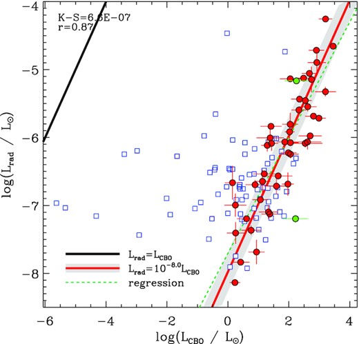
Radio luminosity L_rad as a function of breakout luminosity L_CBO for the split monopole case. The thick black line indicates L_rad = L_CBO; the solid red line shows the same line shifted by the mean difference. The dashed green line shows the regression. Red circles indicate stars with detected emission; blue squares, stars without emission. Green circles indicate HD 171247 and HD 64740.

Open in new tabDownload slide

Equation (14) does not yield quite as high of a correlation coefficient as the purely empirical scaling in Paper I. To see if there is some dependence on the mass-loss rate, the left-hand panel of Fig. 3 shows the residual radio luminosity after subtraction of the monopole L_CBO as a function of bolometric luminosity. There is only a weak dependence on L_bol, with a correlation coefficient r = 0.19 and a slope b = 0.16.

Figure 3.

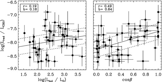
Ratio between L_rad and L_CBO as a function of bolometric luminosity (left) and cos β (right).

Open in new tabDownload slide

Another factor that may affect radio luminosity is the obliquity angle β of the magnetic dipole axis from the rotational axis. Indeed, in the empirical regression analysis in Paper I the factor f_β = (1 + cos β)/2 was found to improve the correlation. The plasma distribution in the CM is a strong function of β, since the densest material accumulates at R_K at the intersections of the magnetic and rotational equatorial planes (Townsend & Owocki 2005). For the special case of an aligned rotator (β = 0^○) this will result in plasma being evenly distributed around R_K. With increasing β the plasma distribution becomes increasingly concentrated at the two intersection points, leading to a warped disc that eventually becomes two distinct clouds. Therefore, the mass confined within the CM will be a maximum for β = 0^○ and a minimum for β = 90^○. If reconnection in the CM is the source of the high-energy electrons that populate the radio magnetosphere, we would then naturally expect that radio luminosity should decrease with increasing β. The right-hand panel of Fig. 3 shows the residual radio luminosity as a function of cos β, and demonstrates that radio luminosity in fact does increase with decreasing β; in fact, the relationship is much stronger than for log L_bol, with r = 0.49 and b = 0.64.

Fig. 4 replicates Fig. 2, with the difference that corrections for |$\dot{M}$| and β are accounted for. Following equation (16), |$\dot{M}$| dependence was determined by scaling equation (14) with |$\eta _{\rm c}^q$|⁠. A purely empirical correction for β was adopted as |$f_{\beta }^x = ((1 + \cos {\beta })/2)^x$|⁠, such that f_β(β = 0^○) = 1 and f_β(β = 90^○) ≠ 0. By minimizing the residuals, the best-fitting exponents are q = −0.09 and x = 2. The former exponent corresponds to p = 1.1, implying only a very slight departure from the monopole scaling. The latter indicates an increase in L_rad by a factor of 4 as β decreases from 90^○ to 0^○. As can be seen in Fig. 4, these corrections lead to a tighter correlation (r = 0.92) and a somewhat reduced ratio between L_CBO and L_rad to around 7 dex.

Figure 4.

As Fig. 2, with L_CBO modified to account for the residual dependence on bolometric luminosity (i.e. the surface mass-flux from the wind) and the tilt angle of the magnetic dipole (Fig. 3).

Open in new tabDownload slide

3.3.1 Emission threshold

Figure 5.

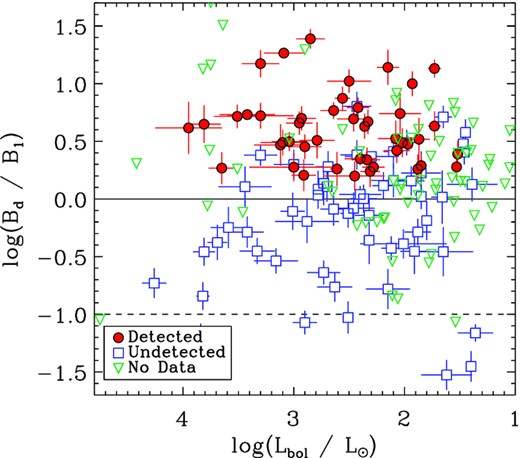
Ratio between surface magnetic field strength and the threshold magnetic field strength necessary to achieve a flux density of 1 mJy, as a function of bolometric luminosity.

Open in new tabDownload slide

As expected, all radio-bright stars have log B_d/B₁ ≳ 0. The relationship for non-detected stars is not as clean as for the similar plot for H α shown by Owocki et al. (2020), as there are a large number of stars with surface magnetic fields above this threshold. However, the radio observations comprising this sample, having been obtained at a variety of observatories with different capabilities over a span of over 30 yr, are quite heterogeneous, with a wide range of upper limits, and many of the non-detected stars in this regime have upper limits comparable to 1 mJy. Further, generally only a single snapshot at one frequency is available, and it is possible that they were observed at inopportune rotational phases. These stars should certainly be reobserved with modern facilities.

The dashed line in Fig. 5 shows the theoretical detection limit for radio telescopes such as the upcoming Square Kilometre Array able to achieve µJy precision, under the assumption that a 10σ detection (i.e. 10 µJy) is necessary for the star’s radio emission to be securely detected. As can be seen, such facilities can at least double the number of stars with measured gyrosynchrotron emission. This is especially true when stars that have not yet been observed in the radio are included: the green triangles in Fig. 5 show those stars from the samples studied by Aurière et al. (2007), Sikora et al. (2019a,b), and Shultz et al. (2019b) without radio observations, essentially all of which are expected to have radio flux densities as above 10 μJy and about half of which should have flux densites above 1 mJy.

3.3.2 How CBO reconnection can lead to radio emission

Breakout events are accompanied by centrifugally driven reconnection of magnetic fields that have been stretched outward by rotational stress acting against the magnetic tension of the initially closed loops. As these loops reconnect, the associated release of magnetic energy can strongly heat the ejected plasma. Some fraction of this reconnection energy can accelerate both ions and electrons to highly superthermal energies, with some of these particles becoming trapped into gyration along closed magnetic field loops near the reconnection site. The associated gyrosynchrotron emission of the much lighter electrons can then produce the observed radio emission.

Regardless of the relative values, a central empirical result here is the finding that L_rad has a clear scaling with rotation frequency as Ω² and with surface field as |$B_{\rm d}^{2/p}$|⁠, dependences which are entirely missing from L_wind. Indeed, we find that log(L_rad) shows only weak correlation with L_wind, with r = 0.3. This strongly disfavours the wind-driven reconnection model proposed by Trigilio et al. (2004); but it is consistent with the scenario proposed here that centrifugal-breakout reconnection provides the underlying energy that leads to the radio luminosity through gyrosynchrotron emission.

While we have cast available energy in terms of loss of the star’s rotational energy, one has to be careful not to take this too literally. Most (70+ per cent) of the angular momentum loss in spin-down is through magnetic field Poynting stresses. But the CBO material that leads to reconnection should share the same basic Weber–Davis scaling with R_A, and it is that component that this scenario associates with the reconnection and the resulting electron acceleration and radio emission.

4 DISCUSSION

4.1 Comparison with alternative theoretical interpretations

The empirical scaling relationship discovered by Leto et al. (2021) and confirmed in Paper I, |$L_{\rm rad} \propto B_{\rm d}^2R_\ast ^4/P_{\rm rot}^2 = (\Phi /P_{\rm rot})^2$|⁠, is explained above as a consequence of electron acceleration via CBO. However, Leto et al. pointed out that Φ/P_rot has the physical dimension of an EMF |$\mathcal {E}$|⁠, which they speculated may be suggestive of an underlying theoretical mechanism. In this section, we examine gyrosynchrotron emission from this standpoint. We perform a theoretical analysis to test if the physical conditions able to sustain large-scale electric currents within the stellar magnetosphere can be verified.

This empirical association by Leto et al. (2021) of radio emission with the voltage of an EMF also stands in contrast with the previous theoretical model by Trigilio et al. (2004), which associates the acceleration of radio-emitting non-thermal electrons with the wind-induced CS that forms in the middle magnetosphere. However, Leto et al. (2021) conclusively demonstrated that the wind does not provide sufficient power to the middle magnetosphere to drive the observed levels of radio emission.

Indeed, equation (21) is very similar to the scaling invoked by Hill (2001, see their equation 4) to model auroral emission from Jupiter. In this case, the magnetospheric EMF accelerates ions and electrons to high energy, which upon penetrating into the underlying Jovian atmosphere is dissipated through the low atmospheric conductance Σ_J (corresponding to high resistivity ρ), resulting in heating and associated thermal bremsstrahlung to give auroral emission.

In contrast, because of the typically very low resistivity of the ionized plasma in hot star magnetospheres, the associated dimensionless Reynolds number is expected to be very large. The associated dissipation luminosity (equation 22) in this EMF scenario would thus be enormous, leading in effect to a ‘short circuit’ that would quickly draw down the available pool of magnetic energy.

In principle, a theoretical model grounded in the EMF could invoke a stronger resistivity in some local dissipation layer, which would enter directly into the predicted scalings for the generated luminosity. But it is unclear how this small-scale dissipation could be reconciled with the large-scale EMF that is taken to scale with the stellar radius, and how such a dissipation could remain fixed over the range of stellar and magnetospheric parameters, in order to preserve the inferred empirical scaling of the observed radio luminosity with the global EMF.

These difficulties with an association of gyrosynchrotron scaling with EMF, and with the CS model, stand in contrast to some key advantages of the CBO mechanism proposed here.

First, this CBO model specifies a more modest magnetic dissipation rate, set by the base dimensional rate |$B_\ast ^2 R_\ast ^3 \Omega$|reduced by the rotation factor W < 1, instead of the enormous Re_rm ∼ 10¹² enhancement of an EMF mechanism. This CBO dissipation can be quite readily replenished over time by the centrifugal stretching of closed magnetic field lines by the constant addition of mass from the stellar wind. As such, the ultimate source of energy thus comes not from the field – which acts merely as a conduit – but from the star’s rotational energy.

Secondly, these eventual CBO events lead naturally and inevitably to magnetic reconnection. This, thus preserves the longstanding notion (Trigilio et al. 2004) that such reconnection provides the basic mechanism to accelerate electrons to high energies, whereupon the gyration along the remaining field lines connecting back to the star results in the gyrosynchrotron emission of the observed radio luminosity.

Thirdly, and perhaps most significantly, instead of the previous notion (Trigilio et al. 2004) that this reconnection is driven by the stellar wind – with no consideration of any role for stellar rotation – our model for CBO-driven reconnection puts rotation at the heart of the process, and so yields a scaling for luminosity that matches the strong dependence on rotation rate, as well as on magnetic field energy. Indeed, while the wind can certainly open the magnetic field and lead to the formation of a CS, this does not itself provide a power source, but merely results in a slower radial decline of the magnetic field strength as compared to that of a dipole. By contrast, CBO provides a clear power source for the acceleration of electrons to high energies.

Thus, although only a small fraction of the breakout luminosity L_CBO ends up as radio luminosity, with an inferred effective efficiency ϵ ≈ 10⁻⁸, the strong correlation between observed and predicted scalings provides strong empirical support for such a CBO model.

4.2 Energy source – magnetic or rotational?

The energy term in equation (14) is B²R³, and it would therefore be natural to assume that the magnetic field is the energy source powering radio emission. However, as suggested in Section 3.2.1, this is probably not the case. The mean magnetic energy E_mag amongst the radio-bright stars is about 10⁴² erg, whereas the mean rotational kinetic energy E_rot in the same sub-sample is about 10⁴⁷ erg, i.e. the star’s rotation is a vastly greater energy reservoir. Indeed E_mag > E_rot for only three stars (HD 46328, HD 165474, and HD 187474), all of which have P_rot ∼ years (and none of which are, of course, detected at radio frequencies).

An additional consideration is that, if the magnetic field were the energy source, radio emission should over time draw down the magnetic energy of the star. The peak radio luminosity is around 10²⁹ erg s⁻¹, implying that the magnetic energy of the most radio-luminous stars would be consumed in about 10¹³ s ∼ 0.3 kyr. To the contrary, fossil magnetic fields are stable throughout a star’s main-sequence lifetime. For Ap/Bp stars below about 4 M_⊙, the decline in surface magnetic field strength is entirely consistent with flux conservation in an expanding stellar atmosphere (e.g. Kochukhov & Bagnulo 2006; Landstreet et al. 2007; Sikora et al. 2019b), while for more massive stars there is an additional, gradual decay of flux (e.g. Landstreet et al. 2007, 2008; Fossati et al. 2016; Shultz et al. 2019b) that is however, much longer than the abrupt field decay time-scale that would be implied if the breakout luminosity was powered by the magnetic field. Furthermore, the most plausible mechanism for flux decay is found in small-scale convective dynamos formed in the opacity-bump He and Fe convection zones inside the radiative envelope (e.g. MacDonald & Petit 2019; Jermyn & Cantiello 2020), which naturally explains why flux does not decay in A-type stars (which lack these convection zones), and why flux apparently decays more slowly for the strongest magnetic fields (Shultz et al. 2019b) since strong fields inhibit convection (Sundqvist et al. 2013; MacDonald & Petit 2019).

In contrast to the magnetic field, which decays slowly or not at all, magnetic braking is quite abrupt (Shultz et al. 2019b; Keszthelyi et al. 2020), making the larger rotational energy reservoirs of rapidly rotating stars a more far more plausible power source. Quantitatively, for the most radio-luminous stars in the sample it would take about 30 Myr for the energy radiated by gyrosynchrotron emission to remove the total rotational energy of the star. For stars with masses above 5 M_⊙ (the mass range of the brightest radio emitters), this is comparable to or greater than the main-sequence lifetime.

It therefore seems that the magnetic field cannot serve as the energy source, but rather acts as a conduit for the extraction of rotational energy and its conversion into gyrosynchrotron emission. The magnetic energy lost in breakout events is immediately replenished as mass is injected into the CM by the wind, with the ion-loaded magnetic field then stretching under the centrifugal stress acting on the co-rotating plasma.

4.3 The case of Jupiter

Leto et al. (2021) showed that the scaling relationship for the non-thermal radio emission from dipole-like rotating magnetospheres also fits the radio luminosity of Jupiter,¹ suggesting an underlying similarity in the physics driving gyrosynchrotron emission from giant planets and magnetic hot stars. Adopting the same parameters as used by Leto et al. (B_eq  = 4 G, P_rot = 0.41 d, M_J = 1.9 × 10²⁷ kg, and R_J = 7.1 × 10⁵ km) gives W = 0.3. The breakout luminosity is then log L_CBO/L_⊙ ∼ −15.9 or, at 1 cm, L_ν ∼ 10⁷ erg s⁻¹ Hz⁻¹, translating to an expected flux density of around 40 Jy at a distance of 4 au. This is about an order magnitude higher than the observed radio luminosity of Jupiter (de Pater & Dunn 2003; de Pater et al. 2003). However, it is worth noting that in the extrapolation shown by Leto et al., Jupiter’s EMF of 376 MV is near the lower envelope of the range of uncertainty inferred from hot stars, i.e. Jupiter is somewhat less luminous than predicted by a direct extrapolation of the hot star scaling relationship. Furthermore, 1 dex is at the upper range of the scatter about the L_CBO relationship (see Figs 2 and 4).

One possible explanation for Jupiter being less luminous than predicted is that Jupiter’s primary ion source, the volcanic moon Io, is effectively a point source offset from the centre of the Jovian magnetosphere. This is in contrast to stellar winds, which feed the magnetosphere isotropically and continuously from the centre. The result is that hot star magnetospheres are relatively more populated, and there is therefore more material available for the generation of gyrosynchrotron emission. Another potential issue is that in the Jovian magnetosphere reconnection takes place in the magnetotail due to stretching by the solar wind; its azimuthal extent will therefore be limited, in analogy to the obliquity dependence found in stellar magnetospheres. Exploring whether the approximate consistency between the Jovian and stellar radio luminosities is indeed due to a similarity in the underlying physics, or is merely coincidental, will require a detailed analysis that is outside the scope of this paper.

4.4 A solution to the low-luminosity problem?

It is notable that magnetospheres are detectable in radio frequencies in stars with CMs that are too small to be detectable in H α. In addition to being a more sensitive magnetospheric diagnostic, this may also suggest an answer to the low-luminosity problem identified by Shultz et al. (2020) and Owocki et al. (2020). While CBO matches all of the characteristics of H α emission from CM host stars, emission disappears entirely for stars with luminosities below about log L_bol/L_⊙ ∼ 2.8. This could be either a consequence of a ‘leakage’ mechanism, operating in conjunction with CBO to remove plasma via diffusion and/or drift across magnetic field lines (Owocki & Cranmer 2018), or due to the winds of low-luminosity stars switching into a runaway metallic wind regime (Springmann & Pauldrach 1992; Babel 1995; Owocki & Puls 2002). In the former case, the leakage mechanism only becomes significant when |$\dot{M}$| is low. In the latter case, H α emission is not produced for the simple reason that the wind does not contain H ions. Notably, the peculiar surface abundances of magnetic stars may lead to enhanced mass-loss rates as compared to non-magnetic, chemically normal stars (Krtička 2014).

Since CBO apparently governs gyrosynchrotron emission, and is seen in stars down to log L_bol/L_⊙ ∼ 1.5, the leakage scenario seems to be ruled out as an explanation for the absence of H α emission. This therefore points instead to runaway metallic winds. One possible complication is that, as is apparent from the direct comparison of H α emission equivalent widths to radio luminosities (see fig. 6 in Paper I), stars without H α so far are also relatively dim in the radio (at least for those stars for which H α measurements have been obtained). These stars have systematically lower values of B_K than have been found in more luminous H α-bright stars (fig. 3 in Paper I). Thus, a crucial test will be examination of both H α and radio for a star with a luminosity well below 2.8, but B_K ∼ 3, i.e. it must be cool, very rapidly rotating (P_rot ∼ 0.5 d), and strongly magnetic (B_d ∼ 10 kG). So far no such stars are apparently known.

Figure 6.

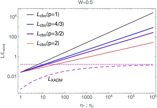
For the standard case of half-critical rotation (W = 0.5), comparison of the X-ray luminosities from the XADM model (dashed) of ud-Doula et al. (2014) with CBO models of various indices p (solid), plotted versus associated magnetic confinement parameter, with all luminosities normalized by the kinetic energy luminosity of the stellar wind, |$L_{\rm wind} = {\dot{M}} v_\infty ^2/2$|⁠. The horizontal dotted line represents the asymptotic luminosity for XADM in the strong-confinement limit. Note that, for this W = 0.5 case, the CBO luminosities are significantly enhanced over that from the XADM model. Results for other rotations can be readily determined by scaling the CBO models with W².

Open in new tabDownload slide

A further complication to the runaway wind hypothesis is provided by 36 Lyn, a relatively cool (T_eff ∼ 13 kK), radio-bright star that, while it does not show H α emission, does display eclipses in H α (Smith et al. 2006) and therefore must have H inside its magnetosphere that, presumably, originated in the stellar wind. Why no other star in 36 Lyn’s T_eff range should show evidence of a similar phenomenon is not currently understood, although its peculiar magnetosphere may be related to the remarkably high toroidal component of its magnetic field in comparison to other magnetic stars, in which the toroidal component is generally quite weak (Oksala et al. 2018; Kochukhov et al. 2019). Alternatively, this may be due to a simple selection effect: 36 Lyn’s eclipses are only detectable for about 10 per cent of its rotational cycle, and eclipse absorption would be broader and shallower for more rapidly rotating stars.

4.5 X-rays from CBO?

The reconnection energy from CBO events might also be important for the X-rays observed from magnetic stars.

For slow rotators with only a DM, and no CM component, the observed X-rays follow quite closely the scaling predicted by the X-rays from analytic dynamical magnetosphere (XADM) model developed by ud-Doula et al. (2014), as shown in fig. 6 of Nazé et al. (2014). With a 10 per cent scaling adjustment to account for the X-ray emission duty cycle seen in MHD simulations, the overall agreement between observed and predicted X-ray luminosities is quite remarkable for such DM stars (denoted by open circles and triangles), spanning more than four orders of magnitude in X-ray luminosity.

However, there are several stars with observed X-ray luminosities well above (by one to two orders of magnitude) the 10 per cent XADM scaling; all are CM stars. These are the very stars that the analysis here predicts to have CBO reconnection events that could power extra X-ray emission, and so supplant the X-rays from wind confinement shocks predicted in the XADM analysis.

To lay a basis to examine whether CBO reconnection X-rays might explain this observed X-ray excess for CM stars, Fig. 6 compares the CBO versus XADM predicted scalings for X-ray luminosity, both normalized by the wind kinetic energy luminosity |$L_{\rm wind} = {\dot{M}} V_\infty ^2/2$|⁠, and plotted versus their associated confinement parameter η_c or η_*. The XADM plot is based on equation (42) of ud-Doula et al. (2014), with velocity exponent β = 1. As seen from equation (18), the CBO scalings also depend on the multipole exponent p, so the various curves show results for various p, as given by the legend. Also, the values shown are for a fixed, fiducial value for the critical rotation fraction W = 1/2, but the results for other rotations can be readily determined by scaling with W².

Note that the CBO scalings increase as |$\eta _{\mathrm{ c}}^{1/p}$|⁠, while the XADM scaling saturates at large η_*. For the chosen default rotation W = 0.5, the CBO scalings are generally above those for the XADM, but this will change for lower W.

To test this possibility that CBO plays a role in augmenting X-ray emission, the next step should be to test whether the observed X-rays from CM stars follow the CBO scaling with η^1/pW², as given by equation (18) when scaled to L_wind, or more generally by equations (12) and (13).

5 SUMMARY AND FUTURE OUTLOOK

The radio luminosities of the early-type magnetic stars were empirically found to be related to the stellar magnetic flux rate (Leto et al. 2021; Paper I). Leto et al. (2021) did not provide a definitive physical explanation regarding the origin of the non-thermal electrons. To provide the theoretical support for explaining how non-thermal electrons originate, in this paper we have extended the CBO model that successfully predicts the H α emission properties of stars with CMs (Owocki et al. 2020; Shultz et al. 2020), deriving a breakout luminosity |$L_{\rm CBO} \propto (B^2R_\ast ^3/P_{\rm rot})W$|⁠, where the first term in parentheses has natural units of luminosity, and the dimensionless critical rotation parameter W is an order-unity correction that includes the additional R_* and P_rot dependence. The radio luminosity is then L_rad = ϵL_CBO, where ϵ ∼ 10⁻⁸ is an efficiency factor. Crucially, there is a nearly 1:1 correspondence between L_rad and ϵL_CBO.

The basic scaling relationship is appropriate for a split monopole. Generalization to higher order multipoles is accomplished with a correction |$\eta _{\rm c}^{1/p}$|⁠, where η_c is the centrifugal magnetic confinement parameter and p is the multipolar order (1 for a monopole, 2 for a dipole, etc.). The small residual dependence of radio luminosity on bolometric luminosity is removed by adopting p ∼ 1.1, i.e. a nearly monopolar field. The minimal residual dependence on L_bol (which in line-driven wind theory sets the mass-loss rate through a scaling |${\dot{M}} \sim L_{\rm bol}^{1.6}$|⁠) confirms that the radio magnetosphere is nearly independent of the mass-loss rate. However, we find that there is a stronger dependence of the residuals on the obliquity β of the magnetic axis with respect to the rotation axis, with L_rad increasing by about a factor of 4 from β = 90^○ to 0^○. This is consistent with expectations from the rigidly rotating magnetosphere model that the amount of plasma trapped in a CM is a strong function of β (Townsend & Owocki 2005), since with less plasma in the CM, there will be fewer electrons available to populate the radio magnetosphere.

While radio emission and H α emission are explained by a unifying mechanism, they probe different parts of the magnetosphere as well as different parts of the CBO process. H α emission probes the cool plasma trapped in the CM, which has not yet been removed by breakout. During a breakout event, some of the energy released by magnetic reconnection accelerates electrons to relativistic velocities, which then return to the star, emitting gyrosynchrotron radiation as they spiral around magnetic field lines. Following the result reported in this paper, we explain the radiation belt model proposed by Leto et al. (2021) to be the magnetic shell connected to the CBO region close to the magnetic equator. This largely preserves the Trigilio et al. (2004) model, with the primary difference being the mechanism of electron acceleration.

Overall, the results here provide a revised foundation on which to build a detailed theoretical model for how centrifugal breakout reconnection leads to acceleration of electrons and the associated radio gyrosynchrotron emission. In particular, we might be able to quantify the level of reconnection heating through MHD simulations, and how it scales with W, η_*, etc., as has been done for other scalings like spin-down.

Future theoretical work should focus on the details of the acceleration of the electrons through reconnection, and their subsequent gyrosynchrotron emission of polarized radio emission (and perhaps other observable spectral bands like X-rays), with the specific aim to understand, and quantitatively reproduce, the inferred emission efficiencies ϵ. This work should also extend to explore the connection with ECM radio emission that has been detected in many of the same stars showing gyrosynchrotron emission (Das et al. 2021).

ACKNOWLEDGEMENTS

MES acknowledges the financial support provided by the Annie Jump Cannon Fellowship, supported by the University of Delaware and endowed by the Mount Cuba Astronomical Observatory. AuD acknowledges support by NASA through Chandra Award 26 number TM1-22001B issued by the Chandra X-ray Observatory 27 Center, which is operated by the Smithsonian Astrophysical Observatory for and on behalf of NASA under contract NAS8-03060. PC and BD acknowledge support of the Department of Atomic Energy, Government of India, under project no. 12-R&D-TFR-5.02-0700.

DATA AVAILABILITY

No new data were generated or analysed in support of this research. All data referenced were part of the associated Paper I.

Footnotes

REFERENCES