


ABSTRACT
The relative velocity between baryons and dark matter in the early Universe can suppress the formation of small-scale baryonic structure and leave an imprint on the baryon acoustic oscillation (BAO) scale at low redshifts after reionization. This ‘streaming velocity’ affects the post-reionization gas distribution by directly reducing the abundance of pre-existing mini-haloes (|$\lesssim 10^7 {\rm M}_{\bigodot }$|) that could be destroyed by reionization and indirectly modulating reionization history via photoionization within these mini-haloes. In this work, we investigate the effect of streaming velocity on the BAO feature in H i 21 cm intensity mapping after reionization, with a focus on redshifts 3.5 ≲ z ≲ 5.5. We build a spatially modulated halo model that includes the dependence of the filtering mass on the local reionization redshift and thermal history of the intergalactic gas. In our fiducial model, we find isotropic streaming velocity bias coefficients bv ranging from −0.0043 at z = 3.5 to −0.0273 at z = 5.5, which indicates that the BAO scale is stretched (i.e. the peaks shift to lower k). In particular, streaming velocity shifts the transverse BAO scale between 0.121 per cent (z = 3.5) and 0.35 per cent (z = 5.5) and shifts the radial BAO scale between 0.167 per cent (z = 3.5) and 0.505 per cent (z = 5.5). These shifts exceed the projected error bars from the more ambitious proposed hemispherical-scale surveys in H i (0.13 per cent at 1σ per Δz = 0.5 bin).
1 INTRODUCTION
One of the main goals of cosmology is to understand the composition of the Universe and how it has evolved over time. General relativity (GR) relates the global properties of the Universe – its mean density and pressure – to the geometry of spacetime. Measurements of the geometry using the luminosity distance to Type Ia supernovae (Riess et al. 1998; Perlmutter et al. 1999) revealed that the expansion of the Universe is accelerating; if interpreted within the framework of GR, this means that the bulk of the cosmic energy density is in the form of ‘dark energy’, which has negative pressure. This discovery has motivated a range of observational programmes to precisely measure the expansion history of the Universe. These programmes aim to measure whether the dark energy density is constant with time (a cosmological constant) or if it is varying, or if there might have been additional components to the cosmic energy budget at higher redshift.
One of the key methods of measuring cosmic geometry uses the baryon acoustic oscillations (BAOs). These are acoustic oscillations in the optically thick photon-baryon plasma that filled the Universe before recombination that are seeded by the initial perturbations. At the time of recombination, the Universe becomes transparent; the baryons, no longer kinematically coupled to the photons, could gravitationally cluster to make large-scale structures. The power spectrum of matter perturbations at low redshift contains oscillations as a function of wavenumber k that are due to the phase of the acoustic oscillation at recombination (Peebles & Yu 1970; Sunyaev & Zel’dovich 1970). These oscillations can be used as a standard ruler, whose length is set by early Universe physics (Eisenstein & Hu 1998; Eisenstein 2002) and can be calibrated using cosmic microwave background (CMB) observations. In a redshift survey, the use of the ‘ruler’ is possible in both the transverse (measurement of distance) and radial (measurement of Hubble rate) directions (e.g. Seo & Eisenstein 2003).
The BAO feature in the distribution of matter can be computed robustly by solving the coupled Einstein, Boltzmann, and hydrodynamic equations of linear perturbation theory (e.g. Ma & Bertschinger 1995) and using N-body simulations to follow the non-linear evolution at low redshift (which leads only to modest changes in the standard ruler length; e.g. Springel et al. 2005). However, the matter density field is not observable directly, particularly since 84 per cent of all matter in the Universe is dark matter (Planck Collaboration I et al. 2020). Instead, we use visible tracers of the matter to measure BAOs. Most of the early measurements of BAOs were performed using massive, mostly red galaxies (e.g. Eisenstein et al. 2005; Anderson et al. 2012, 2014a,b; Padmanabhan et al. 2012; Alam et al. 2017; Beutler et al. 2017; Ross et al. 2017; Gil-Marín et al. 2020; Bautista et al. 2021). Recent measurements have included star-forming galaxies (e.g. Blake et al. 2011; Kazin et al. 2014; Hinton et al. 2017; de Mattia et al. 2021; Raichoor et al. 2021), which have strong emission lines. Emission line galaxies are of particular interest for intermediate redshifts (0.7 ≲ z ≲ 2.5) because the lines tend to be stronger than in the local Universe (z ∼ 0), and the bright lines can be observed with much shorter exposures than would be required to measure the continuum of the galaxies (which is very faint due to the increasing luminosity distance). They will be targeted by ambitious new surveys such as DESI (DESI Collaboration 2016), PFS (Takada et al. 2014), Euclid (Laureijs et al. 2011), and Roman (Spergel et al. 2015). One can also measure the BAO feature using neutral gas: at z > 1.9, the Lyman-α forest is accessible from the ground; BAOs can be measured in the correlation function of the Lyman-α absorption (Busca et al. 2013; Slosar et al. 2013; Bautista et al. 2017; de Sainte Agathe et al. 2019) and in the correlation of this absorption with quasars (Font-Ribera et al. 2013; du Mas des Bourboux et al. 2017; Blomqvist et al. 2019).
Although there is an enormous volume potentially available for BAO studies at high redshifts, 2 ≲ z ≲ 6, upcoming galaxy surveys will only scratch the surface of the cosmological information available there. Individual galaxies become very faint, and their optical emission lines shift farther into the infrared (e.g. H α is beyond the red limit for both the Euclid and Roman space telescopes). The Lyman-α forest provides an alternative approach and has given our current BAO constraints at z ∼ 2.4, but it is sparsely sampled and as one increases the density of sightlines or probes higher redshift, one must go to fainter and fainter sources (McQuinn & White 2011). H i 21 cm emission observed in intensity mapping – that is, in fluctuations in the diffuse background rather than individually detected galaxies – has long been recognized as a powerful way to probe this range (Chang et al. 2008; Wyithe et al. 2008; Morales & Wyithe 2010). Measuring the 21 cm signal is observationally challenging due to the bright foregrounds and consequent need for exquisite control of instrumentation systematics (see, e.g. Shaver et al. 1999 for an early discussion, and Morales et al. 2019 for a recent discussion). But in the meter-wave radio band, it is possible to deploy enormous amounts of collecting area, and the digital signal processing required to calibrate many-element arrays and convert raw data into sky maps is advancing rapidly.
Current H i intensity mapping efforts are focused on the lower redshifts where the foregrounds are fainter. These include chime (Bandura et al. 2014), hirax (Newburgh et al. 2016), tianlai (Chen 2012), fast (Nan et al. 2011), and bingo.1 However, larger experiments probing the higher redshifts have been proposed: the ‘Stage II’ Packed Ultrawide-band Mapping Array (PUMA) reference concept, for example, would be an interferometer composed of 32 000 dishes and probe half the sky out to z ≈ 6 (Ansari et al. 2018). This would saturate most of the BAO information available in that hemisphere, reaching a statistical uncertainty in the BAO scale of 0.13 per cent per Δz = 0.5 bin at 3.5 < z < 5.5.2
This ambitious programme will require both strong control of observational systematics, and an understanding of the astrophysical systematic errors in 21 cm BAO measurements. The BAO feature is famous for being more robust against astrophysical systematics than the broad-band signal, since complicated astrophysical processes are unlikely to produce a narrow feature in the correlation function at a specific scale. However, there is an important exception. The same physics responsible for BAOs also gave baryons a supersonic streaming velocity relative to dark matter at decoupling, which has a feature at the same scale. If the tracer used for BAO analysis retains a memory of the initial streaming velocity, then the BAO feature is distorted and shifted. This leads to an error in the Hubble parameter, H(z), and the angular diameter distance, DA(z), and hence in the inferred expansion history of the Universe. Previous work has explored the impact of streaming velocity in the power spectra of galaxies (Tseliakhovich & Hirata (Dalal et al. 2010; Tseliakhovich & Hirata 2010; Yoo, Dalal & Seljak 2011; Blazek, McEwen & Hirata 2016; Schmidt 2016; Ahn & Smith 2018; Slepian et al. 2018), the Lyman-α forest (Hirata 2018; Givans & Hirata 2020), reionization history (Park et al. 2021), and the pre-reionization 21 cm field (Muñoz 2019; Cain et al. 2020).
This paper presents a first attempt to estimate the streaming velocity effect on post-reionization 21 cm intensity mapping surveys. We focus our attention on the redshift range 3.5 ≲ z ≲ 5.5, i.e. after hydrogen reionization but before the bulk of He ii reionization (and the associated complexities). We consider two major contributions to the streaming velocity bias bv (that is, the fractional change in H i intensity in a region with the root-mean-square (rms) streaming velocity relative to a region with no streaming velocity). The first is the ‘direct’ contribution, in which gas with a different streaming velocity ends up with a different temperature–density relation and a different filtering scale after reionization. The second is the ‘indirect’ contribution, in which the streaming velocity affects the clumping of the gas, and this (locally) changes the reionization history itself. We find the two effects to be of the same order of magnitude, although we estimate the indirect effect to be larger. Our predicted angle-averaged BAO peak shifts range from |$\Delta \alpha = -0.14{{\,\rm per\,cent}}$| at z = 3.5 to |$\Delta \alpha =-0.42{{\,\rm per\,cent}}$| at z = 5.5, which would be significant for an experiment such as PUMA; but we caution that our estimates here represent only a first order-of-magnitude calculation of the BAO peak shift, and we identify possible future improvements.
This paper is organized as follows: In Section 2, we define our formalism and biasing coefficients. In Section 3, we lay out our programme for estimating the various coefficients with a combination of simulations and analytic arguments. The simulations are presented in Section 3, and the results in Section 4. We conclude in Section 5. Some useful formulae for the filtering scale are given in Appendix A.
2 FORMALISM AND CONVENTIONS
2.1 Power spectra
2.2 Perturbation Theory and Biasing Model
Moreover, Givans & Hirata (2020) provides a straightforward pipeline to calculate perturbative corrections to the power spectrum given a set of bias parameters. We therefore adopt their formalism to calculate the H i power spectrum. In Section 3, we present the formalism for calculating input bias coefficients and show how to extract them from hydrodynamics simulations.
2.3 Cosmology
Throughout this work, we use cosmological parameters from the Planck 2015 ‘TT+TE+EE+lowP+lensing + ext’ (Planck Collaboration XIII et al. 2016): Ωm = 0.3089, ΩΛ = 0.6911, Ωbh2 = 0.02230, |$H_0=67.74\,{\rm km\,s^{-1}\,Mpc^{-1}}$|, Yp = 0.249, σ8 = 0.8159, and ns = 0.9667.
3 METHODOLOGY
The post-reionization H i power spectrum could retain a memory of the streaming velocity between dark matter and baryonic matter that existed before recombination. This is possible since streaming velocity affects the H i distribution in two ways. First, the pre-reionization baryonic structure in mini-haloes with mass |$\lesssim 10^7 {\rm M}_{\bigodot }$| is directly suppressed by streaming velocity. Once reionization destroys these mini-haloes, their contents are fed back into the intergalactic medium (IGM). Second, streaming velocity could modulate reionization history via patchy reionization driven by photons within mini-haloes, thereby indirectly modulating the post-reionization matter distribution. Therefore, when constructing our biasing model to calculate the post-reionization H i power spectrum, we should take these two factors into account in the calculation of the streaming velocity biasing coefficient bv.4 As shown in Fig. 1, our work is based on a Gadget-2 simulation of matter evolution. We start by calculating filtering mass MF, which can quantify H i distribution within haloes, to characterize direct effect of streaming velocity. We later account for the indirect effect in the calculation of reionization history. Next, we derive bias coefficients |$b_v, b_1, b_2,\ {\rm and}\ b_{s^2}$| and use them in our H i power spectrum calculation. Finally, we fit the power spectrum to obtain the BAO peak shift Δα due to streaming velocity.

Flow chart from simulation to calculation of BAO scale shift parameter for this work.
In the rest of this section, we describe our model for the calculation of power spectrum in Section 3. We show how to account for direct and indirect streaming velocity effect, respectively, in Section 3.1 and Section 3.2, and then present the equation to obtain the total streaming velocity bias parameter bv in Section 3.3. In Section 3.4, we present the method of calculating other bias parameters |$b_1, b_2, {\rm and}\ b_{s^2}$|. In Section 3.5, we lay out our Gadget-2 hydrodynamics simulations.
To calculate the H i auto-power spectrum accounting for streaming velocity contributions in redshift space, we use the power spectrum model presented in equation (45) of Givans & Hirata (2020). The inputs for the power spectrum calculation are transfer functions, linear matter power spectra, and bias coefficients |${ b_1, b_2, b_{s^2}}$|, and bv. We use CLASS (Blas et al. 2011) to calculate the transfer functions and linear matter power spectrum. The mapping between galaxy bias parameters |$\lbrace b_1, b_2, b_{s^2} \rbrace$| and generalized coefficients {c1…c8} in equation (5) is shown in Givans & Hirata (2020, Table II).
3.1 Direct effect of streaming velocity
In the real Universe, the accreted hydrogen is distributed among several different phases in the interstellar medium and circumgalactic medium of the host, and thus the MHI(Mhalo) relation could differ quite substantially from a strict proportionality with a low-mass cutoff. Normally, this is described with a power-law index α: |$M_{\rm HI}\propto M_{\rm halo}^\alpha$|. At the high-mass end, and at low redshift, group and cluster haloes have less H i than a simple proportionality predicts; the phenomenological high-mass cutoff of Bagla et al. (2010) was used in some early intensity mapping studies, and fits to simulations including AGN feedback give α < 1 at high masses (Villaescusa-Navarro et al. 2016). Additionally, feedback mechanisms could impose a minimum mass greater than the filtering mass MF. In general, we expect the impact of streaming velocities to be enhanced if α < 1 (since more of the H i is in haloes near the filtering mass), but suppressed if, for example, supernova feedback creates an Mmin larger than the filtering mass.
One way to assess the importance of these effects is via hydrodynamic simulations. The MHI(Mhalo) mapping inferred from the IllustrisTNG simulations at z = 4 gives MHI/Mhalo peaking at 0.027 at Mhalo ≈ 1011 h−1 M⊙, decreasing to 0.007 if we go down to Mhalo = 109 h−1 M⊙ (table 1 of Villaescusa-Navarro et al. 2018), a factor of 4 fall-off. However, as seen in fig. 4 of Villaescusa-Navarro et al. (2018), the scatter in the MHI(Mhalo) relation is large, especially at low halo masses; for our purposes, we want the arithmetic average 〈 MHI〉( Mhalo). This is shown in fig. 7 of Villaescusa-Navarro et al. (2018), and 〈 MHI〉/ Mhalo is seen to vary by no more than a factor of 2 (peak-to-valley) from the highest masses all the way down to the filtering mass cutoff at both z = 4 and 5. (We have explicitly checked this using the halo catalogues from Villaescusa-Navarro et al. 2018; for example, at z = 4, 〈 MHI〉/ Mhalo varies from a maximum of 0.32 down to 0.16 at |$M_{\rm halo}=5\times 10^8\, {\rm M}_\odot\,{\rm h}^{-1}$|, just above the filtering mass.) Given this result, we have not chosen to implement a correction to the simple scaling in equation (7).
Filtering masses in units of |$10^7{\rm M}_{\bigodot }\,{\rm h}^{-1}$|.
| zre | vbc | zobs = 5.5 | zobs = 5.0 | zobs = 4.5 | zobs = 4.0 | zobs = 3.5 |
|---|---|---|---|---|---|---|
| 6.0 | On | 0.384 ± 0.003 | 1.715 ± 0.017 | 5.319 ± 0.054 | 12.877 ± 0.133 | 26.246 ± 0.288 |
| Off | 0.147 ± 0.002 | 1.300 ± 0.015 | 4.728 ± 0.047 | 12.130 ± 0.118 | 25.393 ± 0.260 | |
| 7.0 | On | 3.116 ± 0.021 | 7.087 ± 0.047 | 14.043 ± 0.097 | 24.990 ± 0.188 | 40.898 ± 0.337 |
| Off | 2.572 ± 0.015 | 6.421 ± 0.034 | 13.299 ± 0.073 | 24.232 ± 0.147 | 40.210 ± 0.277 | |
| 8.0 | On | 8.162 ± 0.041 | 14.036 ± 0.074 | 22.722 ± 0.130 | 34.887 ± 0.214 | 51.186 ± 0.330 |
| Off | 7.393 ± 0.026 | 13.186 ± 0.050 | 21.804 ± 0.095 | 33.920 ± 0.160 | 50.192 ± 0.245 | |
| 8.5 | On | 10.818 ± 0.051 | 17.326 ± 0.087 | 26.185 ± 0.139 | 38.419 ± 0.209 | 54.794 ± 0.297 |
| Off | 10.117 ± 0.031 | 16.644 ± 0.055 | 25.578 ± 0.093 | 37.943 ± 0.147 | 54.506 ± 0.220 | |
| 9.0 | On | 13.407 ± 0.062 | 20.208 ± 0.096 | 29.378 ± 0.142 | 41.565 ± 0.198 | 57.641 ± 0.265 |
| Off | 12.706 ± 0.036 | 19.555 ± 0.059 | 28.821 ± 0.093 | 41.151 ± 0.134 | 57.417 ± 0.186 | |
| 10.0 | On | 17.607 ± 0.072 | 24.577 ± 0.095 | 33.893 ± 0.120 | 45.777 ± 0.148 | 61.243 ± 0.182 |
| Off | 16.930 ± 0.045 | 23.968 ± 0.061 | 33.380 ± 0.078 | 45.394 ± 0.097 | 61.020 ± 0.122 | |
| 11.0 | On | 21.362 ± 0.068 | 28.678 ± 0.082 | 38.083 ± 0.097 | 49.905 ± 0.114 | 65.498 ± 0.137 |
| Off | 20.653 ± 0.042 | 28.029 ± 0.050 | 37.518 ± 0.059 | 49.446 ± 0.070 | 65.164 ± 0.087 | |
| 12.0 | On | 24.582 ± 0.054 | 32.092 ± 0.061 | 41.405 ± 0.069 | 53.282 ± 0.080 | 68.876 ± 0.098 |
| Off | 23.417 ± 0.202 | 30.908 ± 0.240 | 40.232 ± 0.273 | 52.137 ± 0.303 | 67.758 ± 0.340 |
While total H i is not directly measured at high redshifts, the bias of damped Lyman-α (DLA) absorbers can provide a constraint on the model, since almost all H i is found in damped Ly α systems (DLAs). Péres-Ràfols et al. (2018) find a DLA bias of 1.92 ± 0.20 in their highest redshift bin, 2.5 < z < 3.5. This is consistent with the H i bias b1 that we will infer from equation (7), although one should keep in mind that the linear bias of the DLAs is a single number and so could be consistent with a range of models with other values of the power-law index α and cutoff masses (e.g. Castorina & Villaescusa-Navarro 2017).
3.2 Indirect effect of streaming velocity
The indirect effect of streaming velocity works by modulating the local reionization history, which is traced by the ionized fraction of hydrogen with respect to redshift, xi(z). We follow the approach in D’Aloisio et al. (2020) and Cain et al. (2020) to calculate the reionization history.
3.3 Bias coefficient bv
3.4 Computation of |$b_1, b_2,\ {\rm and}\ b_{s^2}$|
3.5 Simulations and extraction of quantities
We use a modified version of GADGET-2 (Springel, Yoshida & White 2001; Springel et al. 2005), which was used previously in Hirata (2018) for our simulations. All simulations start at the time of recombination, zdec = 1059, with modified initial condition generators to enable or disable streaming velocity between baryons and dark matter. Reionization is implemented by resetting the temperature of gas particles to 2 × 10⁴ instantaneously at zre. Each simulation has the same box size, |$L=1152{\rm \, h^{-1}\, kpc}$|, and the same number of particles, N = 2 × (256)3. This is the same mass resolution that was tested and used in Hirata (2018). All of our simulations were run on the Ruby and Pitzer clusters at the Ohio Supercomputer Center (Ohio Supercomputer Center, Ruby Supercomputer 2015). We archived our modified Gadget-2 N-GenIC files, analysis tools, and tabulated filtering mass data in a Github repository.5
By extracting cs from simulations and then substituting it into the filtering scale calculation, we could get filtering mass and ρHI(zobs, zre). We show filtering masses with discrete zobs in Table 1. The continuous plots for filtering masses are shown in Fig. 2.
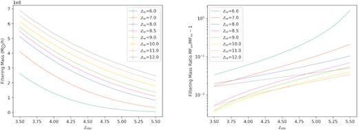
Left-hand panel: filtering mass versus observational redshift zobs. Right-hand panel: the ratio of filtering masses with and without streaming velocity versus zobs.
To obtain reionization history we run simulations with zre ∈ {6, 7, 8, 8.5, 9, 10, 11, 12} and vbc ∈ {0, 33} km s−1. We extract CR from simulations with a cut-off matter density |$\rho \lt 300\overline{\rho }$|, such that ultra-dense regions that could self-shield from being ionized will not be counted in the process of reionization. To carry out the integral in equation (10), we do two-dimensional (2D) interpolations to obtain continuous CR(zre, vbc, zobs) in the range of 8 ≤ zre ≤ 12 and 0 ≤ zre − zobs ≤ 6.0. Note that we interpolate CR in equation (12) in {zre, zre − z} instead of {zre, z} because this way the domain of validity (zre − z > 0) is aligned with the coordinate axes. Also, it is reasonable to interpolate through the time after reionization zre − zobs since the changes of CR for different zre are qualitatively consistent after zre, as shown in Fig. 3.
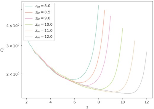
Clumping factors evolution after reionization with zre = 8.0, 8.5, 9.0, 10.0, 11.0, and 12.0. The curves drop right after reionization because of the sudden heat of gases by shocks, and the tails converge since the gases build pressure equilibrium again after they get time to relax.
4 RESULTS
4.1 Filtering masses
We show the filtering masses over the range 6 ≤ zre ≤ 12 and 3.5 ≤ zobs ≤ 5.5 in Table. 1. Streaming velocity suppresses the formation of small-scale structures prior to reionization and leads to larger filtering masses compared to results without streaming velocity. We see that the effect of streaming velocity on filtering mass gradually becomes negligible after reionization while the gas has time to relax. Furthermore, in both cases, filtering masses decrease as zre decreases, since it takes time for the pressure increase at reionization to smooth out small-scale baryonic structure and thereby raise the filtering mass. So, after reionization, the filtering masses grow over time. The quantitative properties of filtering masses MF with respect to zre and zob are also shown in the left-hand panel of Fig. 2. We plot the log of ratio MF with and without streaming velocity in the right-hand panel of Fig. 2.
4.2 Reionization history
We plot the clumping factor CR as a function of redshift z with the reionization redshift zre set from 8 to 12 in Fig. 3. We see that in each case, the clumping factor drops rapidly after reionization because the high-density structures (e.g. filaments and mini-haloes) are disrupted. The gas in these structures flows out into the lower-density IGM. However, as structure growth continues at larger scales, the clumping factor CR begins to increase again. The clumping factor curves converge for different reionization redshifts after the relaxation period.

Top panel: The evolution of ionized hydrogen fraction xi after reionization for zre = 9. Bottom panel: xi difference between simulations with and without streaming velocity.
Summary of different reionization histories.
| zre | zmid | zend | zend, SV − zend, NV | |$\partial x_i/\partial (v^2_{\rm bc}/\sigma ^2)$| | τ | |
|---|---|---|---|---|---|---|
| 9.0 | Fiducial | 7.54 | 6.53 | 0.02 | 0.0092 | 0.059 |
| Delayed | 7.20 | 6.09 | 0.02 | 0.0091 | 0.056 | |
| 12.0 | Fiducial | 8.35 | 6.82 | 0.01 | 0.0080 | 0.065 |
| zre | zmid | zend | zend, SV − zend, NV | |$\partial x_i/\partial (v^2_{\rm bc}/\sigma ^2)$| | τ | |
|---|---|---|---|---|---|---|
| 9.0 | Fiducial | 7.54 | 6.53 | 0.02 | 0.0092 | 0.059 |
| Delayed | 7.20 | 6.09 | 0.02 | 0.0091 | 0.056 | |
| 12.0 | Fiducial | 8.35 | 6.82 | 0.01 | 0.0080 | 0.065 |
4.3 Bias parameters
In Table 3, we list the calculation results of bias parameters b1, b2, |$b_{s^2}$|, and bv over the range 3.5 ≤ z ≤ 5.5. The streaming velocity bias is broken down separately into the direct and indirect effects, bv,dir and bv,ind, calculated using equation (16). We see that bv < 0 by our calculation, indicating that the streaming velocity reduces the H i density, and hence that the BAO ruler stretches because of streaming velocity (Blazek et al. 2016). The absolute value of bv goes down from zobs = 5.5 to 3.5, which is consistent with our interpretation of filtering masses in Section 4.1, i.e. the effect of streaming velocity becomes weaker in lower redshifts. Note that the total streaming velocity bias bv is dominated by bv, dir at higher redshifts. But as redshifts go lower, the contribution from bv, ind becomes more comparable. This indicates that effects of streaming velocity on small-scale structures leave their imprints mainly by directly suppressing the mini-halo abundance, while the memory of ionizing photon sinks modulation is non-negligible when the total streaming velocity memory becomes weaker at lower redshifts.
Bias parameters for three reionization scenarios. The statistical uncertainties of b1, b2, and |$b_{s^2}$| are within 1 per cent. We show the statistical uncertainties of streaming velocity bias parameter from four simulation runs in the table.
| zre | zobs | b1 | b2 | |$b_{s^2}$| | bv | bv, dir | bv, ind |
|---|---|---|---|---|---|---|---|
| 3.5 | 2.2429 | 3.0579 | −0.3551 | −0.0041 ± 0.0005 | −0.0028 ± 0.0006 | −0.0013 ± 0.0001 | |
| 4.0 | 2.3722 | 3.5488 | −0.3921 | −0.0072 ± 0.0006 | −0.0049 ± 0.0007 | −0.0023 ± 0.0001 | |
| 12.0 | 4.5 | 2.4918 | 4.0383 | −0.4262 | −0.0122 ± 0.0006 | −0.0083 ± 0.0008 | −0.0038 ± 0.0002 |
| 5.0 | 2.5976 | 4.5004 | −0.4565 | −0.0195 ± 0.0006 | −0.0136 ± 0.0008 | −0.0059 ± 0.0002 | |
| 5.5 | 2.6888 | 4.9193 | −0.4825 | −0.0272 ± 0.0005 | −0.0213 ± 0.0008 | −0.0058 ± 0.0003 | |
| 3.5 | 2.2210 | 2.9774 | −0.3489 | −0.0043 ± 0.0004 | −0.0032 ± 0.0007 | −0.0010 ± 0.0002 | |
| 4.0 | 2.3374 | 3.4099 | −0.3821 | −0.0076 ± 0.0005 | −0.0057 ± 0.0007 | −0.0019 ± 0.0003 | |
| 9.0 | 4.5 | 2.4391 | 3.8139 | −0.4112 | −0.0130 ± 0.0005 | −0.0097 ± 0.0008 | −0.0033 ± 0.0003 |
| 5.0 | 2.5235 | 4.1660 | −0.4353 | −0.0208 ± 0.0004 | −0.0159 ± 0.0008 | −0.0049 ± 0.0003 | |
| 5.5 | 2.5928 | 4.4629 | −0.4551 | −0.0273 ± 0.0004 | −0.0243 ± 0.0007 | −0.0030 ± 0.0003 | |
| 3.5 | 2.2063 | 2.9247 | −0.3447 | −0.0018 ± 0.0003 | −0.0038 ± 0.0005 | 0.0020 ± 0.0002 | |
| 4.0 | 2.3139 | 3.3200 | −0.3754 | −0.0054 ± 0.0004 | −0.0067 ± 0.0006 | 0.0013 ± 0.0002 | |
| 9.0 (Delay) | 4.5 | 2.4041 | 3.6726 | −0.4012 | −0.0115 ± 0.0003 | −0.0115 ± 0.0006 | −0.0000 ± 0.0003 |
| 5.0 | 2.4761 | 3.9662 | −0.4217 | −0.0199 ± 0.0003 | −0.0185 ± 0.0006 | −0.0014 ± 0.0003 | |
| 5.5 | 2.5403 | 4.2299 | −0.4401 | −0.0241 ± 0.0003 | −0.0257 ± 0.0006 | 0.0017 ± 0.0003 |
4.4 BAO peak shift
Our minimizer uses a Nelder-Mead optimizer to fit the χ2 integral. It explores parameter space to find |$[\, \alpha ,\Sigma \, ]$| and uses least-squares fitting to get associated values of aj and bj. We restrict the minimizer to acceptable regions of parameter space by forcing the integral to return a divergent result if it ventures into prohibited regions. We fit for three different μ values to account for the anisotropic damping of the BAO feature. There is no noise in our fits because the matter power spectra are taken from CLASS and processed through FAST-PT (McEwen et al. 2016; Fang et al. 2017).
Each of the preceding steps is repeated using P21(k, μ) in place of Pbase(k) in equation (24). By taking the best-fitting α when streaming velocity is turned off (Pbase) and subtracting it from the best-fitting α when streaming velocity is turned on (P21), we get a BAO scale shift Δα. Values we calculated for Δα are given in Table 4.
BAO scale shifts as a function of μ and z. We also give the volumes and number densities used in equation (24) since they are functions of redshift.
| zobs | |$V\, [10^{11}\, {\rm h}^{-3}\textrm {Mpc}^3]$| | |$\overline{n}\, [{\{\rm h}^3\textrm {Mpc}^{-3}]$| | μ | Δα per cent |
|---|---|---|---|---|
| 3.5 | 1.8 | 0.030 | 0 | −0.121 |
| |$1/\sqrt{3}$| | −0.135 | |||
| 1 | −0.167 | |||
| 4.0 | 2.2 | 0.033 | 0 | −0.196 |
| |$1/\sqrt{3}$| | −0.220 | |||
| 1 | −0.278 | |||
| 4.5 | 2.5 | 0.033 | 0 | −0.304 |
| |$1/\sqrt{3}$| | −0.317 | |||
| 1 | −0.429 | |||
| 5.0 | 2.8 | 0.031 | 0 | −0.435 |
| |$1/\sqrt{3}$| | −0.486 | |||
| 1 | −0.609 | |||
| 5.5 | 3.1 | 0.028 | 0 | -0.350 |
| |$1/\sqrt{3}$| | −0.395 | |||
| 1 | −0.505 |
Fig. 5 shows how much streaming velocity impacts the H i power spectrum BAO scale. The suppression of power in P21, seen in the trough near |$k=0.04\, {\rm h}\, \textrm {Mpc}^{-1}$|, is more pronounced at higher redshifts. This is consistent with results in Table 4 showing that streaming velocity effects are larger at higher redshifts.

The ratio P21(k)/Pbase(k) based on bias parameters in Table 3. This plot displays results for |$\mu =1/\sqrt{3}$|.
5 CONCLUSION AND DISCUSSION
This work has made a first estimate of the BAO scale shift of post-reionization 21 cm intensity mapping surveys due to the streaming velocity effect. We find that there are two main mechanisms at work. First, there is a ‘direct’ effect: the streaming velocity can modulate the amount of pre-reionization small-scale structure, and the destruction of these structures at reionization affects the thermal state and filtering mass of the intergalactic medium. We found that the streaming velocity raises the filtering masses and hence reduces the amount of neutral gas in haloes following reionization (|$b_{v,\rm direct}\lt 0$|). There is also an ‘indirect’ effect since streaming velocities reduce the clumping factor and thus feedback on the local reionization history itself (Cain et al. 2020) – in this case, accelerating it and increasing the post-reionization filtering mass. This effect is minor at higher redshifts but becomes more comparable to the direct effect at lower redshifts, while imprints of streaming velocity in total have substantially dissipated.
We predict the bias coefficients at redshifts 3.5 ≤ z ≤ 5.5 and find bv < 0, i.e. the BAO scale stretches due to streaming velocity. As one would intuitively expect, |bv| becomes smaller at later times as the thermal and dynamical memory of reionization is erased. The streaming velocity-induced BAO shifts are |$0.167-0.505{{\,\rm per\,cent}}$| in the radial BAO scale and |$0.121-0.350{{\,\rm per\,cent}}$| in the transverse BAO scale. These values may be compared against a precision of 0.13 per cent per Δz = 0.5 bin forecast for the proposed Stage ii 21 cm intensity mapping experiment (Ansari et al. 2018). Although our forecasts are preliminary, this suggests that streaming velocity effects will have to be taken into account in Stage ii or a similar future 21 cm intensity mapping experiment. Two other main sources of theoretical systematics on BAO scale are non-linear evolution of the density field and galaxy formation. These two effects could shift BAO peak from|$0.16{{\,\rm per\,cent}}\ {\rm to}\ 0.11{{\,\rm per\,cent}}$| (Padmanabhan & White 2009) at redshifts 3.5–5.5, which are in the same order of magnitude as streaming velocity effect. Fortunately, these systematics could be substantially reduced by density-field reconstruction as well as further modelling (e.g. Seo et al. 2008; Mehta et al. 2011), so they are not expected to be a limiting systematic.
Our estimates in this paper contain several approximations and simplifications that could be relaxed in future work. We treat photon sinks-modulated reionization history as a local process in our calculation of clumpiness; this is valid as long as the scales of interest (∼|${\pi}$|/k) are larger than the ionization bubbles, but we expect it to break down toward the later stages of reionization. We leave the non-local modelling of how clumpiness modulated by the streaming velocities affects reionization to future work, since it requires a more elaborate simulation (to capture the range of scales, it would require a large box simulation of reionization with subgrid modelling analogous to Ciardi et al. 2006, or use of local clumping factors, e.g. Kohler et al. 2007; McQuinn et al. 2007; Raičević & Theuns 2011, based on the small scale clumping factors appropriate to the streaming velocity in that cell). In this work, we ignore the streaming velocity effect on the star formation rate, while it could suppress the first stars (Pop III) formation and ionizing photon production and then slow down reionization. Cain et al. (2020) investigates this source bias term, but its impact is still unclear because of large modelling uncertainties. A more accurate quantification of this effect requires future studies with a better understanding and modelling of star formation. We have also ignored (Watkinson et al. 2019) X-ray heating prior to reionization, which also reduces the clumpiness of the gas and suppresses small-scale structure. Hirata (2018) found that extreme models of X-ray heating could reduce |bv| for the Lyman-α forest, but future studies should check whether this is also true for post-reionization H i. One should also investigate a wider range of preheating scenarios. Note that we expect some of these potential improvements to the treatment could lower |bv| (e.g. X-ray heating), some could raise |bv| (e.g. streaming velocity modulation of Pop III stars), and for some, it is not clear what direction to expect (e.g. the non-local treatment of reionization). Thus we interpret our calculation as a reasonable first model, but it is not necessarily an upper or lower bound.
Finally, our results motivate further work on mitigation strategies for the BAO peak shift caused by streaming velocities. Previous works (Slepian & Eisenstein 2015; Slepian et al. 2018) have shown that three-point correlation functions could be used to constrain the streaming velocity bias coefficient bv from galaxy survey data. This approach can also help more accurately measure bv in future 21-cm intensity mapping experiments and undo the effect of streaming velocity on the BAO scale. Intensity mapping surveys have the subtlety that the mean brightness temperature |$\bar{T}_{\rm b}(z)$| is not known, which causes a degeneracy for, e.g. growth of structure measurements using redshift space distortions (but see Castorina & White 2019), but upon examining the 3-point formulae in Slepian & Eisenstein (2015) we do not expect a similar issue will arise for bv/b1.
A corrected BAO scale will permit us to better constrain the expansion history of the Universe from redshifts 3.5 ≤ z ≤ 5.5, and bring us closer to understanding dark energy, including any potential early component.
ACKNOWLEDGEMENTS
We thank the anonymous referee, Christopher Cain, Paulo Montero-Camacho, Hee-Jong Seo, and Zachary Slepian for useful comments on the draft. We thank Francisco Villaescusa-Navarro for making available some of the simulated halo catalogues from Villaescusa-Navarro et al. (2016). The authors are supported by NASA grant 15-WFIRST15-0008. This work was partially supported by a grant from the Simons Foundation (#256298 to Christopher Hirata). JG acknowledges additional support from Princeton’s Presidential Postdoctoral Research Fellowship.
This article used resources on the Pitzer Cluster at the Ohio Supercomputing Center.
DATA AVAILABILITY
The filering mass data and analysis tools underlying this article are archived in a Github repository. All the software used in this manuscript are publicly available. Appropriate links are given in the manuscript.
Footnotes
Third-order terms contribute to the 1-loop power spectrum, but if they do not contain the streaming velocity, they will not be part of the streaming velocity correction.
These factors are also important for calculating bvz. However, |bvz| is sufficiently small compared to |bv| that we ignore it in our analysis.
REFERENCES
APPENDIX A: FILTERING SCALE
This calculation extends the calculation of Gnedin (2000), which is equivalent to our result for early decoupling (adec → 0), and for which some analytic fitting functions are available (Kravtsov et al. 2004). Naoz & Barkana (2007) introduced a correction to handle δb/δm not approaching 1 at large scales. There are also extensions for magnetic fields (Schleicher, Banerjee & Klessen 2008; Rodrigues, de Souza & Opher 2010; de Souza, Rodrigues & Opher 2011) and streaming velocities (Naoz et al. 2013; although not treated the same way as in this paper). One can also find some other calculations in the literature, for example an analytic solution for δb/δm in the case of |$c_{\rm s}^2\propto 1/a$| (Nusser 2000).
The filtering scale has contributions both from gas pressure (the sound speed) and from streaming velocities. We consider the sound speed contribution first.
A1 Sound speed
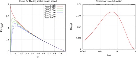
Left-hand panel: The kernel K(ψ; ψdec) of equation (A8), used for the contribution of the sound speed to the filtering length. Right-hand panel: The function Φ(ψdec), used to describe the contribution of streaming velocities to the filtering length.
