


ABSTRACT
We report the discovery of six new magnetar counterpart candidates from deep near-infrared Hubble Space Telescope (HST) imaging. The new candidates are among a sample of 19 magnetars for which we present HST data obtained between 2018 and 2020. We confirm the variability of previously established near-infrared counterparts, and newly identify candidates for PSR J1622−4950, Swift J1822.3−1606, CXOU J171405.7−381031, Swift J1833−0832, Swift J1834.9−0846, and AX J1818.8−1559 based on their proximity to X-ray localizations. The new candidates are compared with the existing counterpart population in terms of their colours, magnitudes, and near-infrared to X-ray spectral indices. We find two candidates for AX J1818 that are both consistent with previously established counterparts. The other new candidates are likely to be chance alignments, or otherwise have a different origin for their near-infrared emission not previously seen in magnetar counterparts. Further observations and studies of these candidates are needed to firmly establish their nature.
1 INTRODUCTION
Magnetars are neutron stars with extremely high magnetic field strengths (B ∼ 1014 G) and are of interest in a wide range of astrophysical research areas (see Kaspi & Beloborodov 2017, for a review). They provide natural laboratories to test quantum mechanics and general relativity at the extremes, have the potential to reveal much about the formation of neutron stars in general, and have been invoked as the central engines in transients ranging from gamma-ray bursts to superluminous supernovae (e.g. Gompertz, O’Brien & Wynn 2014; Metzger et al. 2015; Metzger, Berger & Margalit 2017) and fast blue optical transients (Prentice et al. 2018; Mohan, An & Yang 2020). Recently, they have also been suggested as promising candidates for the origin of extragalactic fast radio bursts (FRBs), a theory backed up by the detection of low-luminosity FRB-like bursts from Galactic magnetar SGR 1935+2154 (Bochenek et al. 2020; CHIME/FRB Collaboration 2020).
A more direct way to study magnetars is to measure the multiwavelength emission from Galactic sources, of which ∼30 are known (Olausen & Kaspi 2014).1 Magnetar emission is distinct from the magnetic dipole braking radiation seen from pulsars – the persistent magnetospheric emission is likely driven by the direct decay of the intense magnetic field (Thompson, Lyutikov & Kulkarni 2002), with bursts and flares driven by magnetic reconnections (akin to solar flares, Lyutikov 2003), starquakes (Thompson & Duncan 1995; Beloborodov & Thompson 2007), or other electrodynamic processes (Heyl & Hernquist 2005). Galactic magnetars are typically discovered through γ-ray/hard X-ray flares, with confirmation following the detection of a coincident persistent X-ray source (or in some cases a radio source, Kaspi & Beloborodov 2017). A population of magnetars has now been identified outside the Milky Way, through the detection of giant flares (Burns et al. 2021).
Other than at γ-ray, X-ray and radio wavelengths, a few magnetars have also been observed in the optical and infrared (e.g. Hulleman, van Kerkwijk & Kulkarni 2004; Kosugi, Ogasawara & Terada 2005; Camilo et al. 2007; Testa et al. 2008; Dhillon et al. 2011; Tendulkar, Cameron & Kulkarni 2012). Given their locations in the Galactic plane, high dust extinctions have restricted these observations, but optical/near-infrared (NIR) variability has been noted in a handful of cases. Sometimes this variability is correlated with X-ray activity (Tam et al. 2004, 2008; Ertan, Göǧüş & Alpar 2006), which can be explained through the presence of a debris disc, formed through supernova fallback, and heated by emission from the magnetar (Ertan & Çalışkan 2006; Wang, Chakrabarty & Kaplan 2006; Özsükan et al. 2014; Tong et al. 2016). Magnetospheric models for the origin of the NIR counterpart also predict a correlation with X-ray emission (Beloborodov & Thompson 2007). However, the NIR and X-rays do not always vary synchronously (Camilo et al. 2007; Testa et al. 2008; Lyman et al. 2022). The aforementioned variability has been reported for a handful of sources over month to year time-scales, but short time-scale (∼seconds) pulsations have also been seen (Kern & Martin 2002; Dhillon et al. 2011).
Studies thus far have been limited by to the small optical/NIR counterpart population size, which has made it difficult to determine whether all magnetars have similar emission properties at these wavelengths. In this paper, we present Hubble Space Telescope (HST) imaging of 19 Galactic magnetars. We perform photometry on previously suggested counterparts and six newly identified candidates reported here for the first time. We compare the magnitudes of the previously known sources to this latest epoch of observations, confirming or establishing NIR variability, and compare the properties of the new candidate counterparts to the existing population.
This paper is structured as follows. We describe the details of the observations and counterpart candidate identification in Section 2, perform photometry in Section 3, and plot the sources on colour–magnitude diagrams in Section 4. The variability and spectral indices of the candidates are discussed in Sections 5 and 6, followed by conclusions in Section 7. Throughout, magnitudes are reported in the Vega system; appropriate conversions from AB magnitudes (Oke & Gunn 1983) have been applied where necessary (either following Blanton & Roweis 2007, or with stsynphot2 for HST filters). The additions to HST Vega magnitudes to obtain AB magnitudes are 0.9204 (F125W), 1.0973 (F140W), and 1.2741 (F160W).
2 OBSERVATIONS AND COUNTERPART IDENTIFICATION
2.1 HST observations
Details of the 19 data sets used in this work are listed in Table 1, along with abbreviated magnetar names that we use throughout. All except CXOU J1647 have F125W (∼J-band) and F160W (∼H-band) imaging, CXOU J1647 has just F140W. All observations were taken with WFC3/IR. There are 20 data sets listed, but guide star acquisition failed for SGR 1806. The previously unpublished images, obtained from the archive, were corrected for charge transfer efficiency (CTE) and reduced with standard drizzlepac procedures (with default settings; Hoffmann et al. 2021). The native pixel scale was maintained, i.e. pixfrac = 1 and final scale 0.1265 arcsec pixel−1. Another source with recent HST observations is SGR 1935. We have not included it here as the data are already published and discussed in detail by Levan, Kouveliotou & Fruchter (2018) and Lyman et al. (2022).
Details of the HST data. Shortened magnetar names (without brackets) are used throughout the paper. The data are primarily from programmes 15348 and 16019 (PI: Levan). The listed exposure times are repeated, once in F160W and once in F125W in each case, with the exception of CXOU J1647 (prog. 14805), for which an F140W exposure was performed twice. WFC3 was used for all observations.
| Magnetar | Prog. | Date | Exp [s] |
|---|---|---|---|
| 4U 0142(+61) | 15348 | 2018 Jan 1 | 598 |
| SGR 0418(+5729) | 16019 | 2020 Jan 29 | 898 |
| SGR 0501(+4516) | 16019 | 2020 Aug 4 | 598 |
| 1E 1547(.0–5408) | 15348 | 2018 Sep 3 | 898 |
| PSR J1622(−4950) | 16019 | 2020 Sep 4 | 898 |
| SGR 1627(−41) | 16019 | 2020 Sep 8 | 898 |
| 1RXS J1708(49.0–400910) | 15348 | 2018 Oct 5 | 898 |
| CXOU J1714(05.7–381031) | 15348 | 2018 Apr 13 | 898 |
| SGR 1745(−2900) | 15348 | 2018 Apr 9 | 898 |
| SGR 1806(−20) † | 15348 | 2018 Jun 18 | 598 |
| XTE J1810(−197) | 15348 | 2018 Aug 3 | 898 |
| Swift J1822(.3–1606) | 15348 | 2018 Jul 5 | 598 |
| SGR 1833(−0832) | 15348 | 2018 Jul 18 | 898 |
| Swift J1834(.9–0846) | 16019 | 2020 Mar 16 | 898 |
| 3XMM J1852(46.6 + 003317) | 15348 | 2018 Jun 14 | 898 |
| SGR 1900(+14) | 16019 | 2020 Aug 26 | 898 |
| 1E 2259(+586) | 15348 | 2018 Aug 16 | 598 |
| SGR 0755(−2933) | 16019 | 2020 Sep 10 | 898 |
| AX J1818(.8–1559) | 15348 | 2018 Aug 2 | 898 |
| CXOU J1647(10.2–455216) | 14805 | 2018 May 23 | 2688 |
Note. † – Guide star not acquired, images unusable.
2.2 Counterpart localization with Chandra
Chandra X-ray Observatory (CXO) observations provide the best localization available for 15 of the 19 magnetars. We download the CXO event files for each source, obtained via the CXO data centre with the Obs IDs as listed in Table 2. Observations are variously with ACIS and HRC. We measure the source positions in these images using the CIAO source detection algorithm wavdetect. Standard ciao (v4.13, with caldb v4.9.3) procedures were used, including reprocessing, PSF map creation and energy filtering to the range 0.5−7 keV (HRC) or 0.5−8 kev (ACIS). Point sources 5σ above the background level are extracted.
Magnetar positions reported in the literature, and details of the CXO-HST alignment described in the text. Where the number of tie sources, Ntie, is listed as X/Y, the first number is the objects matched between CXO and the intermediate, and the second between the intermediate and HST. Refined 2σ uncertainty radii from relative astrometry are listed in the final column, these are used if they provide an improvement over the absolute astrometry, and 2 or more tie objects were available. Where we have been unable to precisely align a CXO X-ray localization on the HST images, we have re-calculated the absolute astrometric uncertainty in these cases using the net source counts from wavdetect and following Evans et al. (2010). These uncertainties are denoted with a † symbol.
| Magnetar | Localization/identification | RA | Dec. | Unc. (enc.) | CXO | Ntie | Intermediate | 2σ unc. |
|---|---|---|---|---|---|---|---|---|
| reference | (as reported) | (as reported) | [arcsec] | Obs ID | [arcsec] | |||
| 4U 0142 | Juett et al. (2002) | 01h46m22|${_{.}^{\rm s}}$|41 | +61d45m03|${_{.}^{\rm s}}$|2 | 0.60 (95)† | 723 | 1 / 61 | Gaia | – |
| SGR 0418 | Van der Horst et al. (2010) | 04h18m33|${_{.}^{\rm s}}$|867 | +57d32m22|${_{.}^{\rm s}}$|91 | 0.35 (95) | 10168 | 0 | Gaia | – |
| SGR 0501 | Göǧüş et al. (2010b) | 05h01m06|${_{.}^{\rm s}}$|76 | +45d16m33|${_{.}^{\rm s}}$|92 | 0.11 (67) | 9131 | 0 | Gaia | – |
| 1E 1547 | Deller et al. (2012) | 15h50m54|${_{.}^{\rm s}}$|12 | −54d18m24|${_{.}^{\rm s}}$|1 | (0.6 × 2) × 10−3 (67) | radio | – | – | – |
| PSR J1622 | Anderson et al. (2012) | 16h22m44|${_{.}^{\rm s}}$|89 | −49d50m52|${_{.}^{\rm s}}$|7 | 0.58 (95)† | 10929 | 2 | None | 0.210 |
| SGR 1627 | Wachter et al. (2004) | 16h35m51|${_{.}^{\rm s}}$|844 | −47d35m23|${_{.}^{\rm s}}$|31 | 0.74 (95)† | 1981 | 3 | None | 0.272 |
| 1RXS J1708 | Israel et al. (2003) | 17h08m46|${_{.}^{\rm s}}$|87 | −40d08m52|${_{.}^{\rm s}}$|4 | 0.7 (95)† | 1936 | 2 | None | 0.502 |
| CXOU J1714 | Halpern & Gotthelf (2010) | 17h14m05|${_{.}^{\rm s}}$|74 | −38d10m30|${_{.}^{\rm s}}$|9 | 0.44 (95)† | 6692 | 2 | None | 0.238 |
| SGR J1745 | Shannon & Johnston (2013) | 17h45m40|${_{.}^{\rm s}}$|16 | −29d00m29|${_{.}^{\rm s}}$|8 | (9 × 22) × 10−3 (67) | radio | – | – | – |
| XTE J1810 | Helfand et al. (2007) | 18h09m51|${_{.}^{\rm s}}$|087 | −19d43m51|${_{.}^{\rm s}}$|93 | 4 × 10⁻³ (67) | radio | – | – | – |
| Swift J1822 | Scholz et al. (2012) | 18h22m18|${_{.}^{\rm s}}$|06 | −16d04m25|${_{.}^{\rm s}}$|5 | 0.58 (95)† | 15992 | 0 | Gaia | – |
| SGR 1833 | Göǧüş et al. (2010a) | 18h33m44|${_{.}^{\rm s}}$|37 | −08d31m07|${_{.}^{\rm s}}$|5 | 0.41 (95)† | 11114 | 2 / 85 | Gaia | 0.588 |
| 3XMM J1852 | Zhou et al. (2014) | 18h52m46|${_{.}^{\rm s}}$|67 | +00d33m17|${_{.}^{\rm s}}$|8 | 2.4 (67) | no CXO | – | – | – |
| SGR 1900 | Frail, Kulkarni & Bloom (1999) | 19h07m14|${_{.}^{\rm s}}$|33 | +09d19m20|${_{.}^{\rm s}}$|1 | 0.4 (95)† | 6731 | 2 / 42 | Pan-STARRS | 0.494 |
| 1E 2259 | Hulleman et al. (2001) | 23h01m08|${_{.}^{\rm s}}$|295 | +58d52m44|${_{.}^{\rm s}}$|45 | 0.38 (95)† | 6730 | 2 / 101 | Gaia | 0.41 |
| SGR 0755 | Doroshenko et al. (2021) | 07h55m42|${_{.}^{\rm s}}$|48 | −29d33m49|${_{.}^{\rm s}}$|2 | 2.0 (97) | 22454 | 1 / 116 | Gaia | – |
| Swift J1834 | Kargaltsev et al. (2012) | 18h34m52|${_{.}^{\rm s}}$|118 | −08d45m56|${_{.}^{\rm s}}$|02 | 0.5 (95)† | 14329 | 0 | Gaia | – |
| AXJ1818 | Mereghetti et al. (2012) | 18h18m51|${_{.}^{\rm s}}$|38 | −15d59m22|${_{.}^{\rm s}}$|62 | 0.51 (95)† | 7617 | 1/148 | Gaia | – |
| CXOU J1647 | Muno et al. (2006) | 16h47m10|${_{.}^{\rm s}}$|20 | −45d52m16|${_{.}^{\rm s}}$|90 | 0.41 (95)† | 19136 | 2 / 188 | Gaia | 0.198 |
As a first step, we attempt to find sources in common between the X-ray and HST images, and compute the offsets in RA and Dec. required to map one set of coordinates to the other (astrometrically ‘tying’ the images). In this way, we are removing the absolute uncertainty of the world coordinate system (WCS) calibrations and are limited only by the relative uncertainty in the transformation. Ideally, we would find sources in common directly between CXO and HST, which was only possible in four cases. The source centroids were measured in each image’s own coordinate system, and the mean RA and Dec. offsets needed to map CXO coordinates on to the HST frame were computed. These were applied to the CXO coordinates, and the RMS difference between the transformed CXO and HST source positions measured. This is added in quadrature to the centroid uncertainty, calculated as FWHM/(2.35 SNR), where FWHM is the full width at half-maximum and SNR is the signal-to-noise ratio. This yields the smallest possible (sub-arcsecond) positional uncertainties. We note that the resulting refined error circle for CXOU J1647 is slightly offset from the source identified as the counterpart by Testa et al. (2008). However, as there are no other objects in the unrefined or refined error circle, we adopt this source as the likely counterpart.
For the remaining 11 sources with HST and CXO observations, there are <2 sources in common that are not a counterpart candidate, precluding a direct tie between HST and CXO (without relying on a single tie object). We instead try to tie the images via an intermediate step. The intermediate image should have an area comparable to CXO images, so that common sources can be found within the CXO field of view, but deep enough for sources in common with HST to be identified. Intermediate catalogues searched include Gaia (EDR3; Gaia Collaboration 2021), 2MASS (Skrutskie et al. 2006), and Pan-STARRS (Chambers et al. 2016). If there were insufficient matches in these surveys, we also searched the ESO and Gemini archives for imaging of the fields. In each case, where Gaia offered enough suitable intermediate tie objects, no improvement could be gained by moving to a different survey. The uncertainty in the CXO-intermediate alignment is calculated in the same way as for the CXO-HST direct alignments, by computing the RA and Dec. shifts required and the RMS of this translation. For the intermediate-HST alignment, there are tens to hundreds of matches, so in principle rotation and scaling could also be left as free parameters. This is equivalent to improving the absolute astrometry of the HST frame. The intermediate (Gaia)-HST RMS values, using simple RA and Dec. shifts, are typically ∼20 mas (e.g. for 1E 2259, 25 mas). This compares well to the RMS values obtained from the FITS headers of HST advanced data product images (for 1E 2259, 23 mas in RA and 26 mas in Dec.), whose astrometric solutions are now calibrated against Gaia (DR1 or DR2) by the automated pipeline. In any case, the CXO-intermediate step dominates the uncertainty in the transformation. Using 1E 2259 as an example again, the CXO-Gaia RMS is 0.2 arcsec, so any further refinement of the HST-intermediate step will be of little benefit.
Details of the image alignment and tying are given in Table 2. Other data sets are available to act as intermediates for 4U 0142 and SGR 0501, but these counterparts are already well established and unambiguously identified. The refined 2σ error radii have three components if an intermediate is used – the two tie steps and the centroid error. Error circles from relative astrometry are drawn as solid circles in Fig. 1, with candidate counterparts (or their expected location in the case of non-detections) indicated by red pointers.
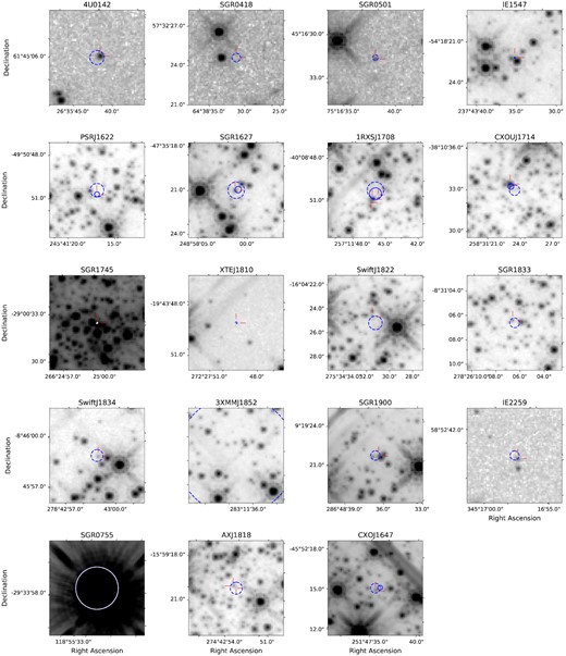
F160W HST imaging of the 19 magnetars (with the exception of CXOU J1647 which has F140W imaging). The cutouts are 8 × 8 arcsec. Error circles that have been refined through relative alignment (e.g. CXO with HST) are drawn as solid lines. Error circles based on absolute astrometry are dashed (if this uncertainty is lower than from relative astrometry, we only show the absolute localization). In each case, the error circle radii are adjusted to enclose ∼95 per cent of the probability. If sources are detected (or have previously been detected) in the error circle, the most likely counterpart position(s) is indicated by red pointers. This location is used to measure a limit in the case of non-detections. If there is no previously reported counterpart, the aperture is placed at the centre of the X-ray error circle. There are three candidates for 1RXSJ 1708, including one outside the error circle which we measure for comparison with Durant & van Kerkwijk (2006a). AXJ 1818 has two candidates. The error circle for 3XMM J1852 is larger than the cutout. For SGRs 0755 and 1745, the error circle is drawn in white for contrast. The corresponding photometry is listed in Table 3.
Where an HST-CXO alignment was not possible even via an intermediate, error circles are placed on the HST images at the coordinates reported by the references in Table 2. The absolute astrometric accuracy of CXO is variously reported in these references as ∼0.6–0.8 arcsec (90 per cent),3,4 but the precise value depends on the source location in the image and net counts. We re-calculate the uncertainty in the absolute astrometry of these sources by taking the net counts from wavdetect and applying the (off-axis angle and source counts dependent) absolute accuracy calculations of Evans et al. (2010). Since many of these sources are bright, and the off-axis angles are exclusively ∼0 (they are the targets), the absolute astrometric uncertainties are typically smaller than previously reported. The sources for which we have performed this calculation are noted in Table 2. If these uncertainties are smaller than those arising from relative alignment, we use the absolute astrometry instead. In one instance, an accurately calculated value is already reported (SGR 0418), and in another, the absolute astrometry of the CXO localization was improved by alignment with 2MASS (SGR 0501).
Two sources have non-CXO localizations plotted in Fig. 1. These are an XMM position for 3XMM J1852 and a Swift/XRT position of SGR 0755 – which we plot instead of the later CXO localization, since this XRT position was associated with the BAT SGR discovery burst. While 3XMM J1852 has CXO observations, they are exclusively in continuous clocking mode, so they cannot be used for imaging. The magnetar is also in the field of view of Kes 79 supernova remnant observations, but is not detected in these images.
When placing positions from absolute astrometry on our HST images, we must also consider that the HST image WCS solutions also have an uncertainty. This is quantified by the RA and Dec. RMS values after source alignment with Gaia as performed by the HST pipeline, of order tens of mas. Assuming the CXO uncertainty is Gaussian, we convert the reported error radius to a 67 per cent radius if it is not already. We add this in quadrature to the HST-Gaia RMS and X-ray centroid uncertainty. In this way, we can derive an approximate 2σ positional uncertainty for the X-ray source in the HST frame. These error circles are drawn with dashed lines in Fig. 1. Measured proper motions for magnetars are at the mas yr−1 level, such that temporal separations between the CXO and HST epochs should only produce small spatial offsets compared to the localization uncertainty.
2.3 Radio localizations
The final three sources in our sample have precise radio localizations. The position of 1E 1547 was measured using very long baseline interferometry observations (Deller et al. 2012). An ellipsoidal uncertainty region of (0.6 × 2.0) mas (1σ) is reported. To place this on the HST frames, however, the uncertainty in the VLBA and HST absolute astrometry must be considered. The quoted VLBA positional error includes both statistical and systematic uncertainties, while the HST frames have been aligned with the Gaia reference frame, with an RMS uncertainty in the HST absolute astrometry of 14 mas (from the RMS|$\_$|RA and RMS|$\_$|DEC header entries). The total uncertainty on the magnetar position in the HST frame is therefore dominated by the HST-Gaia alignment.
Since SGR 1745 lies near the Galactic centre, the extremely high extinction along this sightline means that the chance of any sources seen in the crowded field being associated (rather than foreground objects) is very low. Nevertheless, we can measure a limit at the position on the HST image. As with 1E 1547, we assume the uncertainty on this precise ATCA localization in the HST frame is dominated by the HST WCS solution (Shannon & Johnston 2013). The final magnetar in this sample where we use a radio-localization is XTE J1810. Helfand et al. (2007) report an absolute astrometric uncertainty of 4 mas, so the HST-Gaia WCS solution again dominates.
2.4 Identification through variability
Some NIR counterparts have been identified due to their variability. In these cases, the variable source association is favoured (over non-variable sources in the X-ray error circle) either because the NIR variability correlates with X-ray behaviour, or the expectation that variable NIR sources are sufficiently rare that finding such a source in the error circle by chance is extremely unlikely (although such arguments are as yet poorly quantified).
The source associated with SGR 1900 has H = 21.17 ± 0.04 and Kp = 20.63 ± 0.02 (with 0.5 and 0.1 errors on the zero points), and was suggested as the counterpart due to variability (Tendulkar et al. 2012). The two clear sources within/on the edge of the error circle in the HST imaging presented in Fig. 1 are labelled as sources 3 and 6 by Tendulkar et al. (2012) (and Testa et al. 2008). The suggested variable counterpart, source 7, and another object, source 10, are not readily visible in the HST images, nor are they visible in images re-drizzled on to a 0.065 arcsec pixel−1 grid. To investigate whether proximity to the bright star 3 is obscuring sources 7 and 10 at this resolution, we subtract the PSF of this star in Fig. 2. To do this, we subtract a rotated image cutout centred on star 3, to sample the precise PSF at this location. There is slight excess in the residual image between stars 3 and 6, ∼0.2 arcsec from the centre of star 3, at approximate location of stars 7 and 10 in the Keck/NIRC2 LGS-AO observations of Tendulkar et al. (2012). The reported proper motion of 2.1 ± 0.6 mas yr−1 for the magnetar corresponds to only ∼0.3 pixels of movement over 10 yr at this pixel scale. We conclude that we are not resolving these sources from star 3. The high flux ratio (a magnitude ∼18 source only 0.2 arcsec from magnitude ∼21 sources) makes robust recovery of the suggested counterpart extremely challenging, so we consequently adopt the range of previously reported H and K-band photometry for the suggested variable counterpart (Testa et al. 2008; Tendulkar et al. 2012).
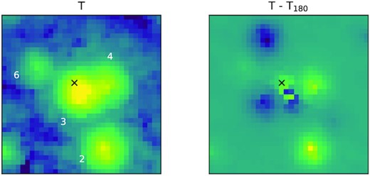
Left: a 2.2 × 2.2 arcsec cutout of the re-drizzled F160W image (pixel scale 0.065 arcsec pixel−1) centred around the target star (T) coincident with SGR 1900 (star 3 of Tendulkar et al. 2012, other sources also follow this labelling). The approximate location of star 7, the SGR 1900 counterpart candidate, is marked by a cross. Right: the target cutout rotated by 180 deg, subtracted from the original cutout. There is a slight excess at the location of sources 7 and 10 in the residual image (mirrored in x and y by an equal deficit since we subtracted a rotated image).
Tendulkar et al. (2012) also identify a candidate counterpart to SGR 1806 thanks to its variability, measuring K ∼ 21.75 ± 0.75 (this approximate uncertainty reflects the source variability), in agreement with Kosugi et al. (2005) who find K = 21.9. We adopt these values since the HST images for this target are unusable following a guide star acquisition failure.
There have been unambiguous localization (both in previous works and here) of magnetar counterparts known to be variable, for example 1E 2259 and 4U 0142 (Hulleman et al. 2004; Tam et al. 2004; Tendulkar, Cameron & Kulkarni 2013). Since they are clearly localized with CXO independent of variability arguments, this demonstrates that at least some magnetar counterparts are variable and supports associations based on variability.
2.5 New counterpart candidates
Using the localizations and imaging described above, we identify counterpart candidates for six magnetars for the first time. These are PSR J1622, Swift J1822, CXOU J1714, Swift J1833, Swift J1834, and AX J1818 (two candidates). This has increased the sample of Galactic magnetar NIR counterparts (confirmed or otherwise) by ∼50 per cent (Olausen & Kaspi 2014). Additionally, SGR 1627 has previous imaging, but the source we deem to be the most likely counterpart has not been measured, as it was too faint for reliable photometry in previous imaging (Wachter et al. 2004). We therefore report photometry for this candidate for the first time.
3 PHOTOMETRY
3.1 Manual photometry
We initially perform manual photometry on counterparts or candidates identified in the 2σ error circles as shown in Fig. 1 and listed in Table 3. Aperture photometry is carried out with the photutils python package (v1.2.0; Bradley et al. 2021). The aperture radius used is typically 0.4 arcsec, but is reduced to as low as 0.1 arcsec if there are immediately neighbouring sources, to reduce flux contamination. The tabulated WFC3 IR encircled energy corrections are applied.5 Because many of these fields are crowded, rather than using an annulus, we estimate the background by placing apertures on ‘blank’ areas of sky (judged by eye) around the image. The background level is extracted by constructing a pixel value distribution from these apertures and using the sigma clipped median.
The HST photometry for candidates in the error circles in Fig. 1, supplemented by H (or if unavailable, K) band data from the literature, where we cannot reliably measure at previously suggested counterpart location. Non-HST data are used for SGR 1900 and SGR 1806 (H and K-band; Tendulkar et al. 2012), and SGR 0755 (H-band, 2MASS). Otherwise, even if we do not detect a previously suggested counterpart, we use the HST photometry as measured below. AXJ 1818 and 1RXSJ 1708 have multiple candidates, the first two for 1RXSJ 1708 follow the same labelling as Israel et al. (2003) and Durant & van Kerkwijk (2006a). Quiescent unabsorbed X-ray fluxes (2–10 kev) are also listed with the reference for the original measurement. Several unabsorbed fluxes were calculated from different energy ranges by Olausen & Kaspi (2014) and they are provided below where the original reference did not give this measurement. In the final column, we give the NIR to X-ray PL index.
| Magnetar | F160W | F125W | Pchance | Unabsorbed FX [2–10 keV] | X-ray reference | NIR to X-ray |
|---|---|---|---|---|---|---|
| (Vega) | (Vega) | [10−12 erg s−1 cm−2] | PL Index | |||
| 4U 0142 | 20.80 ± 0.01 | 21.72 ± 0.01 | 0.000 | 67.9 | Rea et al. (2007b) | 0.98 ± 0.01 |
| SGR 0418 | >25.12 | >26.08 | – | 0.0020|$^{+0.0014}_{-0.0010}$| | Rea et al. (2013) | >0.26 |
| SGR 0501 | 22.56|$^{+0.06}_{-0.07}$| | 23.33 ± 0.07 | 0.002 | 1.7 | Camero et al. (2014) | 0.75 ± 0.02 |
| 1E 1547 | >20.22 | >22.45 | – | 0.54 | Bernardini et al. (2011) | >0.38 |
| PSR J1622 | 22.39 ± 0.05 | 23.95 ± 0.08 | 0.043 | 0.045|$^{+0.063}_{-0.028}$| | Anderson et al. (2012) | 0.33 ± 0.11 |
| SGR 1627 | 20.48 ± 0.01 | 21.97 ± 0.01 | 0.032 | 0.25|$^{+0.17}_{-0.10}$| | An et al. (2012) | 0.32 ± 0.06 |
| 1RXS J1708 (A) | 18.77 ± 0.01 | 20.61 ± 0.01 | 0.036 | 24.3 | Rea et al. (2007a) | 0.66 ± 0.01 |
| 1RXS J1708 (B) | 20.58 ± 0.01 | 22.37 ± 0.02 | 0.104 | – | – | 0.97 ± 0.02 |
| 1RXS J1708 (C) | 21.80 ± 0.08 | 23.71|$^{+0.14}_{-0.16}$| | 0.164 | – | – | 0.85 ± 0.01 |
| CXOU J1714 | 17.45 ± 0.01 | 19.01 ± 0.01 | 0.005 | 2.68 ± 0.09 | Sato et al. (2010) | 0.28 ± 0.01 |
| SGR J1745 | >15.97 | >18.98 | – | <0.013 | Mori et al. (2013) | – |
| SGR 1806 [1] | 21.75 ± 0.75 | – | – | 18 ± 1 | Esposito et al. (2007) | 0.99 ± 0.05 |
| XTE J1810 | >24.79 | >25.58 | – | 0.029 | Gotthelf et al. (2004) | >0.53 |
| Swift J1822 | 19.76 ± 0.01 | 21.04 ± 0.02 | 0.146 | <0.0013 | Scholz et al. (2012) | <-0.34 |
| AXJ1818 (A) | 21.38|$^{+0.14}_{-0.16}$| | 22.80|$^{+0.14}_{-0.16}$| | 0.242 | 1.68|$^{+0.15}_{-0.16}$| | Mereghetti et al. (2012) | 0.63 ± 0.02 |
| AXJ1818 (B) | 20.40 ± 0.06 | 21.87|$^{+0.06}_{-0.07}$| | 0.182 | – | – | 0.53 ± 0.02 |
| 3XMM J1852† | 18.85 ± 0.01 | 21.97 ± 0.02 | 0.948 | <0.001 | Rea et al. (2014) | <−0.47 |
| SGR 1900 [2] | 21.17 ± 0.50 | – | – | 4.8 ± 0.2 | Mereghetti et al. (2006) | 0.74 ± 0.04 |
| IE 2259 | 22.52 ± 0.04 | 23.61 ± 0.05 | 0.016 | 14.1 ± 0.3 | Zhu et al. (2008) | 0.99 ± 0.01 |
| SGR 0755[3] | 9.52 ± 0.01 | 9.69 ± 0.01 | 0.000 | <5.5‡ | Archibald, Scholz & Kaspi (2016) | <-0.31 |
| Swift J1834 | 21.74 ± 0.02 | 23.21 ± 0.03 | 0.050 | <0.004 | Younes et al. (2012) | <-0.01 |
| SGR 1833 | 21.56 ± 0.03 | 22.93 ± 0.02 | 0.031 | <0.2 | Esposito et al. (2011) | <0.41 |
| CXOU J1647 | 22.20|$^{+0.09}_{-0.10}$| (F140W) | – | 0.095 | 0.25 ± 0.04 | An et al. (2013) | 0.48 ± 0.03 |
Notes. † – Reddest source in error circle, not a robust counterpart association. ‡ – 0.5–10 keV.
[1] – K-band photometry from Tendulkar et al. (2012), [2] – H-band from Tendulkar et al. (2012), includes zero-point uncertainty, see Section 2.4.
[3] – HMXB (Doroshenko et al. 2021), listed H and J-band photometry from 2MASS.
To verify this method, we also calculate the background with the photutils function background2D in less crowded fields. In these cases, we get similar results. For example, for the NIR counterpart of 4U 0142, the difference in photometry between aperture background and background2D estimators produce results that differ by much less than the total photometric uncertainty (a 0.008 difference with an error of 0.02). The photometry for the counterparts and candidates is listed in Table 3, with multiple rows where there is more than one candidate. If the flux at the magnetar location fails to reach 3σ significance, a 3σ limit is listed instead.
3.2 Automated photometry
In addition to the aperture photometry, we also perform automated source detection and photometry for all sources in the HST images. There are two reasons for this, (i) to verify the manual measurements and (ii) to obtain magnitudes and colours for every source in the field. This way, we can see if the counterpart candidates stand out as having unusual magnitudes or colours, or find sources that do. dolphot is used (v2.0; Dolphin 2000),6 running on the F160W and F125W bands simultaneously, with the point spread functions of Anderson (2016). Drizzled F160W images are used as the reference, but photometry is performed on the undrizzled flt frames. We retain sources with an SNR of at least 3 in each filter, and reject those with an ellipticity greater than 0.2, helping to remove diffraction spikes and some galaxies. Differences between these measurements and the manual photometry are typically small, but can arise because dolphot accounts for source blending and the PSF, which can have a significant impact on HST photometry in crowded fields (Sodemann & Thomsen 1998).
4 COLOUR–MAGNITUDE DIAGRAMS
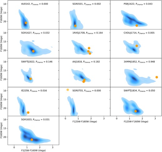
Colour–magnitude diagrams of the fields of the 13 magnetars with dual-band imaging and a detection. The source photometry was extracted in both filters simultaneously using dolphot. The density of field objects in this parameter space is indicated by the blue shading, targets in the error circles in Fig. 1 are shown as orange points (error bars are typically too small to be visible). Unusually red colours, outside the cloud of stellar sources, might indicate a non-stellar origin (e.g. a debris disc); however, this is not necessarily the case: the spectral energy distribution of 4U 0142 suggests the existence of a debris disc, but it does not appear particularly anomalous in this parameter space. The probability of finding a source in the error circle, of the counterpart brightness or brighter, is given by Pchance (the brightest counterpart candidate is used where there are several). The 3XMM J1852 source is simply the reddest object in the large error circle, and is not a robust counterpart candidate.
Searching for unusually red magnetar counterparts is well established, following the discovery that some do have such colours (Wang & Chakrabarty 2002; Israel et al. 2003; Wachter et al. 2004; Durant, Kargaltsev & Pavlov 2011). An infrared excess was confirmed in magnetar 4U 0142, possibly due to a debris disc (Wang et al. 2006). In other magnetars, the red colour may be magnetospheric (Thompson & Duncan 1996). In either case, these sources are non-stellar in colour, appearing distinct from the cloud of other objects. In Fig. 3, most of the counterparts and candidates are not obviously distinct. Even some previously established counterparts are not clearly separated in this J−H versus H parameter space (e.g. 4U 0142; Wang et al. 2006). The magnetars that do have unusual sources in their error circle are CXOU J1714 (off the main sequence), 1RXS 1708 (source A of Israel et al. 2003), 1E 2259 (previously noted as perhaps being magnetospheric in origin; Hulleman et al. 2001), SGR 0755 and 3XMM J1852.
The latter two deserve special attention. For 3XMM J1852, the XMM error circle is nearly 5 arcsec in diameter. There is one exceptionally red source in the error circle, which we adopt as the potential counterpart going forward, with the caveat that there is no way to firmly establish this association with existing data sets.
SGR 0755 has a Swift/XRT localization (indicated on Fig. 1 as this was associated with the BAT discovery burst), and further X-ray observations including a CXO localization (Doroshenko et al. 2021), which is also aligned with the bright star. The Swift/XRT error circle is slightly offset from the centre of the bright star, which cannot be explained by the Gaia proper motion of ∼4 mas yr−1, given that the gap between Swift and HST observations is only 4 yr. In any case, the probability of chance alignment is negligible, and subsequent X-ray observations have also suggested association with the H ∼ 9 Be-star, which has been identified as a high-mass X-ray binary (HMXB; Doroshenko et al. 2021). The source is too bright for HST photometry, so the adopted magnitudes are from 2MASS. The SGR classification was initially due to the Swift/BAT detection of a magnetar-like burst. The HMXB was seen in subsequent Swift/XRT and CXO observations, but is not the sole X-ray source in the ∼3 arcmin BAT error circle, leaving open the possibility of a chance alignment. The 90 per cent uncertainty radius on this localization of ∼3 arcmin is larger than the ∼2 arcmin HST field of view. Although we identify several sources red-wards of the main sequence, there are too many to suggest counterpart candidates (and the magnetar, if not in the HMXB itself, could still lie outside of the field of view).
5 VARIABILITY
In Section 2.4, we discussed the variability of sources in previous observations as an extra tool for identifying counterparts. Counterpart variability is also interesting in its own right, as it can provide clues to the nature of the emission. In Fig. 4, we show the F160W measurements from this paper, compared to previous measurements of the counterpart (H or K-band), where a detection has previously been made (following references in the McGill catalogue, Olausen & Kaspi 2014). We also compare with the candidate detection for CXOU J1647 by Testa et al. (2018), who find J = 23.5 ± 0.2, H = 21.0 ± 0.1, and K = 20.4 ± 0.1. There are cases where we have detected sources below previously established limits, but these are not constraining in terms of variability and so are not shown. Where there is only K-band data to compare, it is difficult to establish if there is variability, or simply a red H−K colour (not unusual for magnetars).
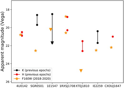
The seven magnetars for which we identify (or place limits on) a previously known NIR counterpart (excluding SGR 1935; see Lyman et al. 2022, for a discussion of the variability of this source). Shown are the F160W measurements (this work; note that CXOU J1647 has F140W observations instead), compared with H-band, or if unavailable, K-band data from previous studies.
Four have previous ∼H-band observations, and a long baseline between observations (4U 0142, previous observed from 2004–2006, 1RXSJ 1708, previously observed 2006, XTEJ 1810, previously observed 2007–2008 and CXOU J1647, previously observed 2013). For 1RXSJ 1708, the second (fainter) source is added from just outside the error circle (labelled star B; Durant & van Kerkwijk 2006a). The H-band magnitudes of stars A (the brightest object) and B are reported by Durant & van Kerkwijk (2006a) to be 18.82 ± 0.06 and 20.29 ± 0.13. We report magnitudes of 18.77 ± 0.01 and 20.58 ± 0.01, respectively. The star A measurements are therefore consistent, while star B has a ∼2.2σ difference. Given the proximity of star A to star B, and the difference between the H and F160W filters, this is unlikely to be a reliable variability measurement. None the less, Durant & van Kerkwijk (2006a) claim the potentially variable star B as the more likely counterpart based on its anomalous JHK colours.
4U 0142 is consistent with previously noted variability (Hulleman et al. 2004; Durant & van Kerkwijk 2006b), and there are significant differences between our measurements of SGR 0501 and 1E 2259, although these are also in different bands. CXOU J1647 appears to have faded by ∼1 mag, but the most striking change is in XTEJ 1810 that has dropped ∼2.5 mag (a factor of ∼10 in flux). This is much more than the previously reported H-band variability of this source (∼1 mag; Testa et al. 2008). If the NIR emission is thermal in nature (flux ∝ T4), as in the case of blackbody emission from a debris disc, this corresponds to cooling by a factor of ∼2 over a 10 yr time-scale.
Variability of NIR emission can equally be explained if we invoke a surviving binary companion as the origin of the emission. The variability of stars in the NIR is poorly understood (e.g. Levesque & Massey 2020), but such a scenario would predict a lack of correlation in the variability seen for different spectral bands in some magnetars. Roughly equal-mass binaries would be likely to place OB-stars as the companions, which can have prominent variability in the NIR (Bonanos et al. 2009; Roquette et al. 2020). Another possibility, given the young age estimates for magnetars, are pre-main-sequence companions. These could feasibly remain pre-main sequence for longer than the lifetime of a massive star magnetar progenitor, and are known to be variable in the NIR (e.g. Carpenter, Hillenbrand & Skrutskie 2001; Eiroa et al. 2002; Alves de Oliveira & Casali 2008). We will investigate these possibilities further in a separate paper (Chrimes et al., in preparation).
6 NIR–X-RAY SPECTRAL INDICES
Another measurement we can make for the sample, placing the new candidate counterparts in context, is the NIR to X-ray spectral index. We fit a power law (PL) between the unabsorbed quiescent X-ray flux, adjusted so that all measurements are in the ∼2–10 keV range (taken from Olausen & Kaspi 2014, where necessary), and F160W (or nearest available band, see Table 3). The corresponding frequencies used are 9 × 10¹⁷ Hz and 2 × 10¹⁴ Hz, with νFν ∝ ν1 − β and β = 1 − Γ. The uncertainties are not quantified for all of the X-ray flux estimates, where they are not, a 10 per cent uncertainty is assumed, with the caveat that this may be an underestimate.
We first note that the six sources reported here for the first time have typical apparent magnitudes compared to the existing population, with 17.5 < H < 22.5 (see Table 3). Most notable is SGR 0755, which is by far the brightest source at H ∼ 10. However, there is ambiguity as to whether this Be-star HMXB is associated with SGR 0755, in which case the accretor would be the magnetar, or whether this is an unrelated HMXB which happened to lie in the 3 arcmin error region of the Swift/BAT discovery burst (Doroshenko et al. 2021).
Fig. 5 shows the cumulative distribution of PL indices Γ. Previously established counterparts – those for which a single source has previously been noted due to unambiguous localization or variability – include 4U 0142, SGR 1900, SGR 1806, 1E 2259, SGR 0501, CXOU J1647, and XTE 1810. There is a clear delineation between these known counterparts and the new candidates – all known sources lie at the upper end of the distribution. The lowest (CXOU J1647) has Γ = 0.43, the only new candidates to lie above this are for AX J1818.
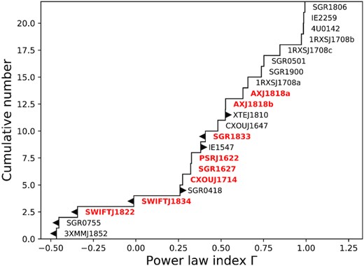
The cumulative distribution of NIR to X-ray PL indices (Table 3). Sources for which we report a counterpart candidate for the first time are labelled in bold/red, limits are indicated on the corresponding histogram step. Photon index upper limits are due to X-ray upper limits, and lower limits are NIR non-detections. Only SGR 1745 (not plotted) lacks a quiescent detection in both the NIR and X-ray and therefore has an unconstrained Γ. The new candidates have lower indices than previously established counterparts, with the exception of AX J1818.
To measure these indices, we have used unabsorbed X-ray fluxes and observed NIR fluxes, uncorrected for extinction. Magnetars with previously established NIR counterparts have relatively low extinction estimates (e.g. Av ∼3.5 for 4U 0142; Wang et al. 2006). The neutral hydrogen column density assumed to calculate the unabsorbed quiescent X-ray flux of 4U 0142 is 1022 cm−2 (Rea et al. 2007b). This corresponds to an extinction of AV ∼ 5 according to the AV−NH relation inferred from X-ray scattering haloes and supernova remnants (Predehl & Schmitt 1995). The unabsorbed X-ray estimate is therefore broadly consistent with a small NIR extinction correction of ∼0.6 mag, given Av ∼3.5, a Fitzpatrick extinction curve (Fitzpatrick 1999) and Rv = 3.1. This further implies that the PL of index of ∼1 for 4U 0142 is close to the intrinsic, unattenuated value. Similar arguments can be made for other established counterparts, such as 1E 2259 and SGR 0501.
Although extinction is generally low at NIR wavelengths, magnetar sightlines are frequently in the plane of the Galaxy where even NIR extinctions can be large. However, this cannot reconcile the lower PL indices of the new counterparts with previously established ones: correcting for NIR extinction would only increase the NIR flux and decrease the indices, pushing them further from the existing population. Assuming that intrinsic indices of 0.5–1 are typical, this suggests that the new candidates reported here are either chance alignments or are fundamentally different in nature to the other counterparts. This could include, for instance, bound companion stars, a possibility which we will explore in a subsequent paper (Chrimes et al., in preparation).
A possible exception is AX J1818, for which the two candidates in the error circle both have Γ values similar to known counterparts. The likely explanation is that one of the sources is the genuine counterpart, and the other is a brighter, bluer object at a larger distance with more extinction, such that it appears to have a similar magnitude and colour. There is a similar situation for 1RXS J1708, which has three similar (in terms of Γ) candidates in the error circle. To determine whether this is a likely scenario by chance, we consider both the magnitude and colour of the AX J1818 candidates. We first note that the Pchance values (based on F160W magnitudes only) are high for these sources, at 0.32 and 0.24. Secondly, in terms of F125W-F160W colours, the AX J1818 values of ∼1.45 are typical for the field: 17 per cent of sources in the HST images have redder colours, and 83 per cent are bluer. Therefore, it is not improbable to find chance alignments within the error circle which happen to have a similar appearance to genuine counterparts.
Although not part of this HST sample, we also calculate the NIR–X-ray spectral index for the possible Galactic FRB source SGR 1935. Using a quiescent X-ray flux level of ∼5 × 10⁻¹¹ erg s−1 cm−2, and HST measurement of mF140W ∼ 25 (Lyman et al. 2022), we find that this object has Γ ∼ 1.2. Although this is the highest value in the population, the steep, positive slope is similar to other established counterparts.
At the extreme low end of the PL index distribution are SGR 0755, possibly an unrelated HMXB as discussed, and 3XMM J1852, for which we simply selected the reddest source in the large error circle. If NIR–X-ray spectral indices of 0.5–1 are typical of genuine magnetar counterparts, this suggests that simply searching for anomalously red objects may be not a reliable method of identification.
Going forwards, spectral energy distributions constructed from photometry will be needed, if not spectra, to reliably separate magnetar counterparts from other sources in the field. This can also be seen in Fig. 3, where the counterparts do not always stand out from other sources. Counterpart spectral energy distributions should be constructed using data taken as close to simultaneously as possible, given that these sources can be highly variable, as demonstrated by Fig. 4.
7 CONCLUSIONS
In this paper, we have measured the magnitudes and colours of Galactic magnetar counterpart candidates in deep HST imaging, adding a later epoch for several sources, and confirming their variability on 5–10 yr time-scales. We identify six new NIR counterpart candidates for SGR J1622−4950, Swift J1822.3−1606, CXOU J171405.7−381031, Swift J1833−0832, Swift J1834.9−0846, and AX J1818.8−1559. This represents a substantial ∼50 per cent increase in the NIR counterpart sample size. Placing these new candidates in the context of the wider population, we find that they have typical apparent magnitudes but lower NIR–X-ray indices, with the exception of the AX J1818 candidates. This implies either that the new candidates are chance alignments, or that the emission mechanisms are distinct from previously established counterparts. To make further progress in identifying and understanding these counterparts, more data points are needed across the optical/NIR, since two-band colours are not necessarily enough to distinguish them from other sources. It is important for such observations to be taken as close together in time as possible, as magnetar counterparts can be highly variable over time-scales of months and years, and the inferred properties could vary substantially if different epochs are combined.
ACKNOWLEDGEMENTS
AAC was supported by the Radboud Excellence Initiative. AJL had received funding from the European Research Council (ERC) under the European Union’s Seventh Framework Programme (FP7-2007-2013) (Grant agreement No. 725246). PJG acknowledges support from the NRF SARChI program under grant no. 111692. JDL acknowledges support from a UK Research and Innovation Fellowship (MR/T020784/1). CK and ASF acknowledge support for this research, provided by NASA through a grant from the Space Telescope Science Institute, which is operated by the Association of Universities for Research in Astronomy, Inc.
Support for this research was provided by NASA through a grant from the Space Telescope Science Institute, which is operated by the Association of Universities for Research in Astronomy, Inc. Observations analysed in this work were taken by the NASA/ESA Hubble Space Telescope under programs 14805, 15348 and 16019.
This work has made use of ipython (Perez & Granger 2007), numpy (Harris et al. 2020), scipy (Virtanen et al. 2020); matplotlib (Hunter 2007), astropy,7 a community-developed core python package for Astronomy (Astropy Collaboration 2013; Price-Whelan et al. 2018) and photutils, an astropy package for detection and photometry of astronomical sources (Bradley et al. 2021). We have also made use seaborn packages (Waskom 2021).
This research has made use of the SVO Filter Profile Service (http://svo2.cab.inta-csic.es/theory/fps/) supported from the Spanish MINECO through grant AYA2017-84089 (Rodrigo, Solano & Bayo 2012; Rodrigo & Solano 2020).
This research has made use of software provided by the Chandra X-ray Center (CXC) in the application of the ciao package.
This publication makes use of data products from the Two Micron All Sky Survey, which is a joint project of the University of Massachusetts and the Infrared Processing and Analysis Center/California Institute of Technology, funded by the National Aeronautics and Space Administration and the National Science Foundation.
This work has made use of data from the European Space Agency (ESA) mission Gaia (https://www.cosmos.esa.int/gaia), processed by the Gaia Data Processing and Analysis Consortium (DPAC, https://www.cosmos.esa.int/web/gaia/dpac/consortium). Funding for the DPAC has been provided by national institutions, in particular the institutions participating in the Gaia Multilateral Agreement.
Finally, we thank the anonymous referee for their constructive comments regarding the astrometry and clarity of this manuscript.
DATA AVAILABILITY
Based on observations made with the NASA/ESA Hubble Space Telescope, obtained from the data archive at the Space Telescope Science Institute. STScI is operated by the Association of Universities for Research in Astronomy, Inc. under NASA contract NAS 5-26555. These observations are associated with programs 14805, 15348, and 16019 (Levan). The scientific results reported in this article are based on data obtained from the Chandra Data Archive.
