


ABSTRACT
We present a detailed study of the highly obscured active galaxy NGC 4507, performed using four Nuclear Spectroscopic Telescope Array (NuSTAR) observations carried out between May and August in 2015 (∼130 ks in total). Using various phenomenological and physically motivated torus models, we explore the properties of the X-ray source and those of the obscuring material. The primary X-ray emission is found to be non-variable, indicating a stable accretion during the period of the observations. We find the equatorial column density of the obscuring materials to be ∼2 × 1024 cm−2 while the line-of-sight column density to be ∼7–8 × 1023 cm−2. The source is found to be deeply buried with the torus covering factor of ∼0.85. We observe variability in the line-of-sight column density on a time-scale of <35 d. The covering factor of the Compton-Thick material is found to be ∼0.35 in agreement with the results of recent X-ray surveys. From the variability of the line-of-sight column density, we estimate that the variable absorbing material is likely located either in the BLR or in the torus.
1 INTRODUCTION
Active galactic nuclei (AGNs) are classified as Type-1 and Type-2, based on the presence or absence of broad optical/UV emission lines. The simplified unification model of AGNs can explain different types of AGN based on different inclination angles with respect to an obscuring torus (Antonucci 1993). In this framework, the Type-2 AGNs are seen edge-on (i.e. through the obscuring torus), while the Type-1 AGNs are observed face-on. Work carried out in the infrared has shown that the molecular torus is likely clumpy, rather than uniform (e.g. Nenkova et al. 2008a,b). The level of obscuration towards the X-ray source is typically parametrized with the hydrogen column density (NH).
Over the years, many AGNs are observed to show variable NH in a time-scale of hours to years (Risaliti, Elvis & Nicastro 2002). The short-term variations (on time-scales of ∼days) are believed to be associated with the broad-line emitting region (BLR), while the long-term variability (on time-scales of months to years) are believed to be caused by the clumpy molecular torus (Markowitz, Krumpe & Nikutta 2014). A growing number of AGNs, e.g. UGC 4203 (Risaliti et al. 2010), NGC 4151 (Puccetti et al. 2007), NGC 2992 (Weaver et al. 1996; Murphy, Yaqoob & Terashima 2007), IC 751 (Ricci et al. 2016), NGC 6300 (Guainazzi 2002; Jana et al. 2020), have shown variable NH by repeated X-ray observation. In recent years, a new sub-class of AGNs, known as changing-look AGN has emerged. In these objects, the line of sight column density can go from a Compton-thin (NH < 1024 cm−2) to a Compton-thick state (CT; NH > 1024 cm−2) level, or vice versa. These events can lead to a dramatic change in the observed X-ray spectrum, which can go from being reflection dominated (in the Compton-thick state) to transmission dominated (in the Compton-thin state), or vice versa (Guainazzi 2002; Matt, Guainazzi & Maiolino 2003). These events are believed to be an important confirmation of the clumpiness of the BLR or torus (Guainazzi 2002; Elitzur 2012; Yaqoob et al. 2015; Jana et al. 2020).
NGC 4507 is a nearby (z = 0.0118) barred spiral galaxy, classified as SAB(s)ab (Tueller et al. 2008; Winter et al. 2009). NGC 4507 is reported to be one of the brightest (|$F_{\rm 2-10}^{\rm obs} \sim 10^{-11}$| erg cm−2 s−1) Seyfert 2 galaxies in the hard X-ray band (>10 keV; Braito et al. 2013), and was detected by INTEGRAL/ISGRI, Swift/BAT and CGRO/OSSE (Bassani et al. 1995; Ricci et al. 2017a). Over the years, several X-ray studies have revealed a variable NH in the range of ∼1–9 × 1023 cm−2 based on the observations by Ginga, ASCA, BeppoSAX, XMM–Newton, and Chandra (Awaki et al. 1991; Comastri et al. 1998; Risaliti 2002; Matt et al. 2004; Marinucci et al. 2013).
In this paper, we present a detailed X-ray spectral analysis of NGC 4507, obtained with four NuSTAR observations carried out between 2015 May and August, with a total exposure time of ∼130 ks. We aim to probe the variability of the obscuration from these broad-band X-ray observations. The paper is structured as follows. In Section 2, we present the data extraction procedure. The timing analysis is reported in Section 3. In Section 4, we report our detailed spectral analysis and our results. In Section 5, we discuss our findings, and compare them to previous studies. Finally, in Section 6, we summarize our findings.
2 OBSERVATION AND DATA REDUCTION
NuSTAR observed NGC 4507 four times between 2015 May and August with an interval of about five weeks between the different observations. In this work, we studied all NuSTAR observations in an energy range of 3–60 keV (see Table 1). NuSTAR is a hard X-ray focusing telescope, consisting of two identical modules: FPMA and FPMB (Harrison et al. 2013). Data were reprocessed with the NuSTAR Data Analysis Software (NuSTARDAS, version 1.4.1). Cleaned event files were generated and calibrated by using the standard filtering criteria in the nupipeline task, and the latest calibration data files available in the NuSTAR calibration data base.1 The source and background products were extracted by considering circular regions with 90 arcsec radii, centred at the source coordinates and away from the source, respectively. The spectra and light curves were extracted using the nuproduct task. We re-binned the spectra to ensure that they had at least 20 counts per bin by using the grppha task.
Log of the NuSTAR observations of NGC 4507 studied here.
| ID | UT Date | Observation ID | Exp (s) | Count s−1 |
|---|---|---|---|---|
| N1 | 2015-05-03 | 60102051002 | 30133 | 0.736 ± 0.005 |
| N2 | 2015-06-10 | 60102051004 | 34464 | 0.773 ± 0.005 |
| N3 | 2015-07-15 | 60102051006 | 32225 | 0.743 ± 0.005 |
| N4 | 2015-08-22 | 60102051008 | 30924 | 0.720 ± 0.005 |
3 TIMING ANALYSIS
We generated light curves in different energy ranges to study the variability in NGC 4507. Fig. 1 shows the light curves in 3–60 keV energy range for observations N1, N2, N3, and N4. We calculated the fractional rms variability (Fvar) to study the variability of the source (Nandra et al. 1997; Edelson et al. 2002; Vaughan et al. 2003). During the observation N1, we obtained Fvar < 5 per cent in 3–10 keV energy range. We did not observe any variability in 3–10 keV energy range in other observations. No variability was observed in 10–60 keV and 3–60 keV energy ranges. We also calculated the fractional rms variability in ∼35 d time-scale. We found the fractional rms variability, |$F_{\rm var} \lt 3{{\ \rm per\ cent}}$| in 35 d time-scale.
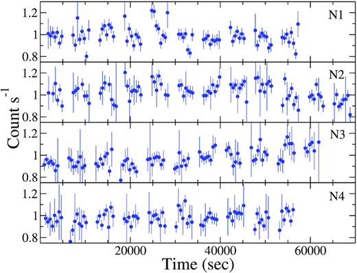
Light curves of NGC 4507 in 3–60 keV energy ranges for the observation N1, N2, N3, and N4. Each points represent 500 s.
4 SPECTRAL ANALYSIS
We carry out the spectral analysis in the 3–60 keV energy range in XSPEC v12.102 (Arnaud 1996). For the spectral analysis, we used various spectral models, based on slab and torus geometries. In all models, we included phabs component for the Galactic absorption with abundances set to those of Anders & Grevesse (1989) and considered the photoelectric absorption cross-section of Verner et al. (1996). We fixed the Galactic column density to NH = 6.8 × 1020 cm−2 (HI4PI Collaboration 2016). We set the cosmological parameters to H0 = 70 km s−1 Mpc−1, Λ0 = 70, σM = 0.27 (Bennett et al. 2003). We calculated uncertainties of all spectral parameter at the 90 per cent confidence level (1.6 σ).
4.1 Slab model
Here, phabs1 represent the Galactic absorption in the direction of the source. This model (hereafter the slab model) provided a good fit for all observations. The results show that the X-ray source is highly obscured during all observations, with NH varying in the range 6.3 ± 0.4–7.6 ± 0.6 × 1023 cm−2. The photon index was found to be roughly constant (Γ ∼ 1.6−1.7). The cut-off energy (Ecut) was obtained to be constant (|$E_{\rm cut} \sim 121^{+107}_{-41}-135^{+58}_{-73}$| keV) within the uncertainty. We detected strong Fe Kα line emission in all four epochs, with an equivalent width (EW) of 237 ± 7 eV, 203 ± 7 eV, 235 ± 8 eV, and 233 ± 8 eV in observations N1, N2, N3, and N4, respectively (see Table 1). The reflection was found be moderate (Rrefl ∼ 0.4). The results obtained with this model are reported in Table 2. To test if the variability of NH is real and not associated with a degeneracy with the continuum parameters (Γ and Ecut), we fitted all the spectra simultaneously with Γ and Ecut tied together. Using this approach, we found a similar variability of NH. We show the best-fitted unfolded spectra obtained with the slab model in the left-hand panel of Fig. 2, while the corresponding residuals are shown in the right-hand panel of Fig. 2. In the left-hand panel of Fig 2, the black, red, green, and blue solid lines represent the best-fitted slab model for N1, N2, N3, and N4, respectively, while the black, red, green, and blue point represents the data for the observation N1, N2, N3, and N4, respectively. Fig. 3 shows the confidence contour between the photon index (Γ) and line of sight column density (NH).
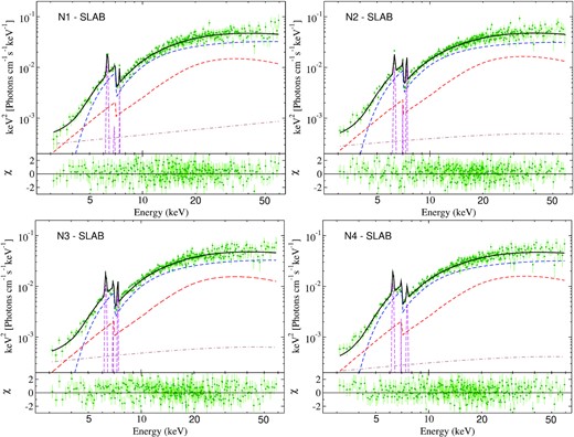
Unfolded spectra fitted with the slab model for observations N1 (top left), N2 (top right), N3 (bottom left), and N4 (bottom right). Upper panel: Green points represent the data. The black, blue, red, magenta, and brown lines represent the total emission, primary emission, reprocessed emission, line emission (Fe Kα, Fe Kβ, and Ni Kα), and scattered primary emission. Bottom panel: Corresponding residuals.
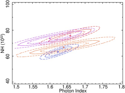
Confidence contour between the photon index (Γ) and line-of-sight column density (NH) in 1022 cm−2, fitted with the slab model. The red, blue, magenta, and orange lines represent the observation from N1, N2, N3, and N4, respectively. The dot–dashed, solid, and dashed lines represent the contours at 1σ, 2σ, and 3σ level, respectively.
The slab model fitted spectral analysis result.
| N1 | N2 | N3 | N4 | ||
|---|---|---|---|---|---|
| (1) | |$N_{\rm H}^{\rm los}$|(1023 cm−2) | |$7.6^{+0.5}_{-0.6}$| | |$6.3^{+0.5}_{-0.5}$| | |$7.4^{+0.5}_{-0.4}$| | |$6.7^{+0.3}_{-0.5}$| |
| (2) | Γ | |$1.65^{+0.06}_{-0.05}$| | |$1.62^{+0.05}_{-0.04}$| | |$1.61^{+0.05}_{-0.05}$| | |$1.64^{+0.07}_{-0.06}$| |
| (3) | Ecut (keV) | |$121^{+107}_{-41}$| | |$126^{+61}_{-37}$| | |$114^{+62}_{-21}$| | |$135^{+58}_{-73}$| |
| (4) | NPL (10−2 ph cm−2 s−1) | |$2.20^{+0.06}_{-0.04}$| | |$1.76^{+0.07}_{-0.08}$| | |$1.88^{+0.10}_{-0.09}$| | |$1.82^{+0.07}_{-0.06}$| |
| (5) | Rrefl | |$0.38^{+0.08}_{-0.12}$| | |$0.46^{+0.14}_{-0.23}$| | |$0.29^{+0.10}_{-0.14}$| | |$0.41^{+0.13}_{-0.24}$| |
| (6) | fScat (10−2) | |$0.97^{+0.04}_{-0.03}$| | |$0.97^{+0.02}_{-0.02}$| | |$1.21^{+0.02}_{-0.02}$| | |$0.81^{+0.02}_{-0.02}$| |
| (7) | Fe Kα LE (keV) | |$6.38^{+0.04}_{-0.04}$| | |$6.35^{+0.04}_{-0.04}$| | |$6.37^{+0.04}_{-0.03}$| | |$6.33^{+0.06}_{-0.05}$| |
| (8) | EW (eV) | |$237^{+6}_{-7}$| | |$203^{+6}_{-7}$| | |$235^{+6}_{-8}$| | |$233^{+7}_{-8}$| |
| (9) | Norm (10−4 ph cm−2 s−1) | |$3.15^{+0.93}_{-0.68}$| | |$2.15^{+0.42}_{-0.61}$| | |$2.93^{+0.45}_{-0.62}$| | |$2.61^{+0.45}_{-0.68}$| |
| (10) | Fe Kβ LE (keV) | |$6.99^{+0.09}_{-0.07}$| | |$7.08^{+0.05}_{-0.06}$| | |$6.98^{+0.09}_{-0.07}$| | |$7.04^{+0.07}_{-0.08}$| |
| (11) | EW (eV) | <24 | <26 | <31 | <23 |
| (12) | Norm (10−6 ph cm−2 s−1) | |$2.06^{+1.04}_{-1.24}$| | |$1.91^{+1.02}_{-0.88}$| | |$4.34^{+1.01}_{-0.97}$| | |$3.87^{+1.53}_{-2.13}$| |
| (13) | Ni Kα LE (keV) | |$7.47^{+0.10}_{-0.07}$| | |$7.45^{+0.17}_{-0.13}$| | |$7.45^{+0.11}_{-0.16}$| | |$7.62^{+0.07}_{-0.10}$| |
| (14) | EW (eV) | <48 | <35 | <32 | <105 |
| (15) | Norm (10−5 ph cm−2 s−1) | |$8.77^{+1.34}_{-1.53}$| | |$2.38^{+1.35}_{-1.43}$| | |$1.83^{+0.71}_{-0.88}$| | |$10.01^{+1.45}_{-1.85}$| |
| (16) | χ2/dof | 632/590 | 620/625 | 615/613 | 567/586 |
| (17) | |$F_{\rm 2-10}^{\rm obs}$| (10−11 erg cm−2 s−1) | |$0.96_{-0.03}^{+0.03}$| | |$1.06_{-0.03}^{+0.02}$| | |$0.94_{-0.03}^{+0.04}$| | |$0.99_{+0.02}^{-0.01}$| |
| (18) | |$L_{\rm 2-10}^{\rm intr}$| (1043 erg s−1) | |$3.70_{-0.15}^{+0.18}$| | |$3.23_{-0.15}^{+0.17}$| | |$3.62^{+0.14}_{-0.16}$| | |$3.30^{+0.12}_{-0.14}$| |
| (19) | |$L_{\rm 0.1-100}^{\rm intr}$| (1044 erg s−1) | |$1.21_{-0.02}^{+0.03}$| | |$1.04_{-0.03}^{+0.02}$| | |$1.24_{-0.03}^{+0.04}$| | |$1.10_{-0.03}^{+0.04}$| |
| (20) | LKα (1042 erg cm−2 s−1) | |$0.99_{-0.07}^{+0.09}$| | |$0.95_{-0.07}^{+0.08}$| | |$0.97_{-0.12}^{+0.10}$| | |$0.96_{-0.10}^{+0.08}$| |
Note. (1) Line-of-sight hydrogen column density (|$N_{\rm H}^{\rm los}$|) in 1023 cm−2, (2) photon index (Γ) of the primary emission, (3) cut-off energy (Ecut) in keV, (4) power-law normalization (NPL) in 10−2ph cm−2 s−1, (5) reflection fraction (Rrefl), (6) fraction of scattered primary emission (fScat), (7) Fe Kα line energy in keV, (8) equivalent width of the Fe Kα line in eV, (9) normalization of the Fe Kα line in 10−4 ph cm−2 s−1, (10) Fe Kβ line energy in keV, (11) equivalent width of the Fe Kβ line in eV, (12) normalization of the Fe Kβ line in 10−6 ph cm−2 s−1, (13) Ni Kα line energy in keV, (14) equivalent width of the Ni Kα line in eV, (15) normalization of the Ni Kα line in 10−5 ph cm−2 s−1, (16) χ2 value for degrees of freedom (dof), (17) 2–10 keV observed flux |$F_{\rm 2-10}^{\rm obs}$| in 10−11 erg cm−2 s−1, (18) 2–10 keV intrinsic luminosity |$L_{\rm 2-10}^{\rm intr}$| in 1043 erg s−1, (19) 0.1–100 keV intrinsic luminosity (|$L_{\rm 0.1-100}^{\rm intr}$|) in 1044 erg s−1, (20) Fe Kα line luminosity (LKα) in 2–10 keV energy ranges in 1042 erg cm−2 s−1.
4.2 MYTORUS
The pexrav model considers reflection from a semi-infinite slab. Hence, it might not provide an accurate representation of the reprocessed radiation in obscured AGN. Thus, to probe the complex absorber, one should consider a more physical torus model. For our spectral analysis, we used the physically motivated torus model mytorus3 (Murphy & Yaqoob 2009; Yaqoob 2012). This model consists of an absorbing torus, surrounding the X-ray source, with a fixed opening angle of 60○ (i.e. a covering factor of 0.5). mytorus has three spectral components: the zeroth ordered component (MYTZ), a scattered/reprocessed component (MYTS), and a line component (MYTL). The MYTZ component describes the absorbed transmitted continuum emission in the line of sight. The MYTS component describes the reprocessed emission from the surrounding torus. The relative normalization (AS) of the MYTS component is estimated using a ‘constant’ in XSPEC. The MYTL component describes the Fe Kα and Fe Kβ line emission. The relative normalization of this component (AL) is set to be the same as the relative normalization (AS) of the MYTS component. Any deviation of AS from unity could indicate a time-delay between MYTZ and MYTS components, or indicate different geometries of the material with different NH, or a torus covering factor different than 0.5 (Yaqoob 2012). The mytorus model can be used in two configurations: coupled (MYTC) and decoupled (MYTD). The coupled configuration describes an uniform torus, while the decoupled configuration could be used to describe a clumpy torus (Yaqoob 2012).
4.2.1 Coupled configuration
In this model, the photon index (Γ), equatorial hydrogen column density (|$N_{\rm H}^{\rm Eq}$|), inclination angle (i) and normalization of MYTS and MYTL components are tied to those of the MYTZ component. As recommended, the relative normalization of MYTS and MYTL components are tied, i.e. AS = AL. The photon index and normalization of the scattered component (zpowerlaw2) are tied to those of the primary continuum (zpowerlaw1). We also added a Gaussian component for Ni Kα line emission, and used a Gaussian convolution model gsmooth to convolve the MYTL component.
The line-of-sight column density (|$N_{\rm H}^{\rm los}$|) is found to be |$7.5^{+4.2}_{-2.2}$|, |$6.5^{+2.7}_{-1.4}$|, |$8.1^{+2.9}_{-1.9}$|, and |$6.5^{+2.4}_{-1.4} \times 10^{23}$| cm−2 for the N1, N2, N3, and N4 observation, respectively. The photon index was obtained to be roughly constant (Γ ∼ 1.7). The relative normalization (AS) was observed to deviate from unity in all four observations, indicating delayed reprocessed emission or different geometries of the absorbing material with different NH, or a different geometry from that assumed by mytorus. The parameters obtained by using this model are reported in Table A1. Fig. B1 shows the best-fitting spectrum obtained with the MYTC model. The confidence contours between |$N_{\rm H}^{\rm Eq}$| and Γ are shown in Fig. C1.
Variation of line-of-sight column density (|$N_{\rm H}^{\rm los}$|), obtained from different models.
| ID | Slab | MYTC | MYTD | borus02 | xclumpy | RXTorus |
|---|---|---|---|---|---|---|
| N1 | |$7.6^{+0.5}_{-0.6}$| | |$7.5^{+4.2}_{-2.2}$| | |$8.2^{+1.3}_{-1.3}$| | |$9.4^{+0.6}_{-0.6}$| | |$8.1^{+2.4}_{-1.5}$| | |$6.9^{+2.4}_{-1.6}$| |
| N2 | |$6.3^{+0.5}_{-0.5}$| | |$6.5^{+2.7}_{-1.4}$| | |$7.0^{+1.4}_{-1.3}$| | |$8.3^{+0.7}_{-0.6}$| | |$7.0^{+1.6}_{-1.1}$| | |$6.0^{+0.9}_{-1.1}$| |
| N3 | |$7.4^{+0.5}_{-0.4}$| | |$8.1^{+2.9}_{-1.9}$| | |$8.1^{+1.5}_{-1.5}$| | |$9.8^{+0.6}_{-0.6}$| | |$8.2^{+1.6}_{-2.3}$| | |$7.0^{+1.6}_{-1.8}$| |
| N4 | |$6.7^{+0.3}_{-0.5}$| | |$6.5^{+2.4}_{-1.4}$| | |$7.1^{+1.3}_{-1.4}$| | |$8.4^{+0.5}_{-0.5}$| | |$7.1^{+1.5}_{-2.2}$| | |$6.1^{+1.5}_{-2.1}$| |
Note. |$N_{\rm H}^{\rm los}$| is in unit of 1023 cm−2.
4.2.2 Decoupled configuration
The spectral analysis, performed with the MYTD model, provided a good fit for all observations. We found, however, that the averaged column density of the obscured materials (|$N_{\rm H}^{\rm tor}$|) varied in the range of ∼1.9–2.4 × 1023 cm−2. Within the observation period of ∼4 months, the global obscuration properties is unlikely to change. Thus, we fitted all four spectra simultaneously with |$N_{\rm H}^{\rm tor}$| tied together, and obtained |$N_{\rm H}^{\rm tor}$||$=2.2^{+0.6}_{-0.5} \times 10^{23}$| cm−2. The line-of-sight column density varied in the range of 7.0 ± 1.4–8.2 ± 1.3 × 1023 cm−2. The detailed spectral analysis result using MYTD model is given in Table A2. MYTD model fitted unfolded spectra are shown in Fig. B2. Fig. C2 shows the confidence contour between |$N_{\rm H}^{\rm tor}$| and |$N_{\rm H}^{\rm los}$| for all observations, fitted with MYTD.
4.3 Borus02
zphabs2*cabs*zcutoffpl1 represents the absorbed direct primary emission. ‘const1’ represents the relative normalization (AS) of the reprocessed component. const2*cutoffpl represents the scattered primary emission while const2 is the scattering fraction (fScat). The photon index (Γ), cut-off energy (Ecut), normalization of cutoffpl1, zcutoffpl2, and borus02 model are linked together. The column densities of cabs and zphabs2 models are tied together, and represents the line-of-sight column density obscuration.
We simultaneously fitted all four spectra with borus02 model with |$N_{\rm H}^{\rm tor}$|, inclination angle (i), iron abundance (AFe), and torus covering factor (Ctor) tied together. First, we fitted the spectra with a fixed cut-off energy at Ecut = 400 keV and iron abundance at Solar value (AFe = 1). We allowed the cut-off energy to vary, and the fit improved by Δχ2 = 8 for 1 dof. The fit improved significantly (Δχ2 = 34 for 1 dof) when we allowed the Fe abundance (AFe) to vary, which resulted in a sub-Solar value in all four observations, with AFe ∼ 0.47 ± 0.07. We found a column density of the obscuring material of |$N_{\rm H}^{\rm tor}$||$=2.6^{+0.7}_{-0.6} \times 10^{23}$| cm−2. The line-of-sight column density was found to be |$9.4^{+0.6}_{-0.6} \times 10^{23}$|, |$8.3^{+0.7}_{-0.6} \times 10^{23}$|, |$9.8^{+0.6}_{-0.6} \times 10^{23}$|, and |$8.4^{+0.5}_{-0.5} \times 10^{23}$| cm−2 for N1, N2, N3, and N4, respectively. We obtained the inclination angle to be |$i = 64.5^{+5.2}_{-6.3}$|°. The torus covering factor is found to be Ctor = 0.58 ± 0.10 with the torus opening angle to be obtained in the range of ∼47°–60°. The results obtained with this fit are reported in Table A3. borus02 model fitted unfolded spectra are shown in Fig. B3. The confidence contour between |$N_{\rm H}^{\rm tor}$| and |$N_{\rm H}^{\rm los}$| is shown in Fig. C3 for all observations, fitted with borus02.
4.4 XCLUMPY
The first term is the direct primary emission. The second and third terms represent the reprocessed and line emission, respectively. The last term represents the scattered primary emission. The parameters of xclumpy|$\_$|R and xclumpy|$\_$|L models are linked. The photon index (Γ), cut-off energy (Ecut), and normalization of xclumpy|$\_$|R model are linked with the cutoffpl1. The const1 and const2 represent the relative normalization of the line emission (AL) and scattering fraction (fScat).
We fitted all the four spectra simultaneously using the xclumpy model, with |$N_{\rm H}^{\rm Eq}$| and i tied together. We fitted the spectra with cutoff energy fixed at Ecut = 370 keV, since the xclumpy table consider a fixed cut-off energy at 370 keV. We found that the inclination angle is |$i = 64.1^{+7.4}_{-4.9}$|°, while the equatorial column density is |$N_{\rm H}^{\rm Eq}$|= |$2.1^{+0.6}_{-0.9} \times 10^{24}$| cm−2. The line-of-sight density was obtained to be, |$N_{\rm H}^{\rm los}$|= |$8.1^{+2.4}_{-1.5}\times 10^{23}$|, |$7.0^{+1.5}_{-1.2} \times 10^{23}$|, |$8.2^{+1.5}_{-2.2} \times 10^{23}$| and |$7.1^{+1.5}_{-2.1} \times 10^{23}$|, for N1, N2, N3, and N4, respectively. The torus angular width we obtained is roughly constant with σtor ∼ 25–26°. The results of this spectral analysis are reported in Table A4. Fig. B4 shows the xclumpy model fitted unfolded spectra. Fig. C4 shows the confidence contour between the |$N_{\rm H}^{\rm Eq}$| and σtor, fitted with the xclumpy model.
4.5 RXTORUS
We fitted all four spectra simultaneously with the inclination angle and equatorial column density tied together. The normalization of the primary emission and rxtorus|$\_$|rprc components are tied together. The equatorial column density is found to be |$N_{\rm H}^{\rm Eq}=2.1^{+0.6}_{-0.5} \times 10^{24}$| cm−2, while the line-of-sight column density varied between |$\sim 6.0^{+0.9}_{-1.1} - 7.0^{+1.6}_{-1.8} \times 10^{23}$| cm−2. The covering factor (r/R) was obtained to be ∼0.41−0.42. The results of the spectral analysis are presented in Table A5. Fig. B5 shows the RXTorus model fitted unfolded spectra. The confidence contour between the |$N_{\rm H}^{\rm Eq}$| and σtor is shown in Fig. C5.
5 DISCUSSION
We presented the detailed spectral analysis result of NGC 4507 using NuSTAR observations in 3–60 keV energy range. We carried out the spectral analysis with the slab model, mytorus, borus02, xclumpy, and RXTorus models.
5.1 Comparison among different spectral models
Using the results obtained by our X-ray spectral analysis, we explore the nuclear and obscuration properties of NGC 4507. The main difference among different spectral models is how they treat the reprocessed emission. While pexrav assumed reflection from a cold, semi-infinite slab, physically motivated torus-based model assumed different torus structures and geometries. Therefore, the fits performed using the different models return slightly different results. As the absorber is likely not uniform, given the column density variability found here and in previous works (e.g. Braito et al. 2013), we do not discuss the results obtained considering the MYTC model.
The spectral analysis carried out using different models resulted in different values of Γ. The slab model, MYTD, xclumpy, and RXTorus models returned with Γ ∼ 1.6−1.7, while the borus02 model indicated slightly flatter spectra with Γ ∼ 1.5. For all models, the photon index was roughly constant across the different observations.
The variation of |$N_{\rm H}^{\rm los}$| was observed to be similar as obtained from different spectral models. The slab model showed that |$N_{\rm H}^{\rm los}$| varied in the range of ∼6–8 × 1023 cm−2, while MYTD and xclumpy showed that |$N_{\rm H}^{\rm los}$| varied in the range of 7–9 × 1023 cm−2. The RXTorus, borus02, and xclumpy models also returned with similar value of |$N_{\rm H}^{\rm los}$|, varying in the range of ∼6–9 × 1023 cm−2. The |$N_{\rm H}^{\rm los}$| variation, obtained from different spectral model, is listed in Table 3.
5.2 Nuclear properties
Our spectral analysis indicated very little variation of the photon index during the observations, and the parameter can be considered constant within the uncertainties. The cut-off energy is found to be in the range of |$E_{\rm cut} \sim 121^{+107}_{-41}~{\rm keV}-135^{+58}_{-73}$| keV from the slab model and |$75^{+29}_{-15}-97^{+46}_{-18}$| keV from borus02 model. This is consistent with typical values found for nearby AGN (e.g. Ricci et al. 2018; Baloković et al. 2020). Both models indicate a constant cut-off energy within our observations. The intrinsic luminosity in the 2–10 keV energy band is found to be in the range of |$L_{\rm 2-10}^{\rm intr} \sim (3.0\pm 0.2 - 3.6\pm 0.3) \times 10^{43}$| erg s−1. Vasudevan & Fabian (2009) estimated the bolometric correction factor κbol, 2–10 keV ≈ 15–30 for λEdd > 0.1, and κbol, 2–10 keV ≈ 10 for λEdd ≤ 0.1. Considering the bolometric correction factor κbol, 2–10 keV = 20, we obtained, the bolometric luminosity in the range of Lbol = (5.9 ± 0.4–7.2 ± 0.5) × 1044 erg s−1. The Eddington ratio would be λEdd = Lbol/LEdd ∼ 0.1, considering the black hole mass, MBH = 4.5 × 10⁷ M⊙ (Marinucci et al. 2012). However, Winter et al. (2009) reported of a higher mass (MBH ∼ 108.4 M⊙), which would lead to λEdd ∼ 10−1.7. Even, if we consider κbol ∼ 10, λEdd would be 10−2. Regardless the assumption of mass or bolometric factor, the Eddington ratios of the source is consistent with that of nearby Seyfert galaxies (Wu & Liu 2004; Koss et al. 2017).
5.3 Obscuration properties
From the spectral analysis, we obtained several torus parameters, such as the line-of-sight column density (|$N_{\rm H}^{\rm los}$|; from the slab model, MYTC, MYTD, borus02, and xclumpy), the averaged column density of the obscuring materials (|$N_{\rm H}^{\rm tor}$|; from MYTD and borus02), the equatorial column density (|$N_{\rm H}^{\rm Eq}$|; from MYTC, xclumpy and RXTorus), and the torus covering factor (CFtor or θtor; from borus02, xclumpy & RXTorus). We obtained similar variations of |$N_{\rm H}^{\rm los}$| from different spectral models (see Section 5.1). The equatorial column density (|$N_{\rm H}^{\rm Eq}$|) was found to be ∼2.1 ± 0.6 × 1024 cm−2, whereas the line of sight column density was found to be ∼6–8 × 1023 cm−2.
For |$N_{\rm H}^{\rm los}$|= 1022 cm−2, we obtained corresponding elevation angle, θ = 56°– 61°. This transforms to the torus covering factor Ctor = sin θ ∼ 0.83–87. Considering Compton-thick obscuration, i.e. setting |$N_{\rm H}^{\rm los}$|= 1024 cm−2 in equation (4), we obtained a covering factor |$C_{\rm tor}^{\rm T} \sim 0.34-0.37$|. Our X-ray spectral analysis with the borus02 and RXTorus models returned Ctor ∼ 0.6 and ∼0.4.
Ricci et al. (2017b) showed that the radiation pressure from the AGN could efficiently expel dusty gas when λEdd ≳ 10−1.5. They showed for the Compton thin material (NH = 1022–24 cm−2), a high covering factor is observed (Ctor ∼ 0.85) for 10−4 ≤ λEdd ≤ 10−1.5, while a much lower covering factor (Ctor ∼ 0.4) is observed for λEdd ≥ 10−1.5. On the other hand, for the Compton-thick material (NH > 1024 cm−2), the covering factor is predicted to be |$C_{\rm tor}^{\rm T} \sim 0.2-0.3$| (see also Ricci et al. 2015). We obtained an Eddington ratio of λEdd ∼ 0.1 for MBH ∼ 107.65 M⊙ (Marinucci et al. 2012). Our estimated torus covering factor is Ctor ∼ 0.85 which is higher than the predicted value for λEdd ∼ 0.1. However, if we consider a higher mass, MBH = 108.4 M⊙ (Winter et al. 2009), the Eddington ratio is λEdd ∼ 10−2. For this Eddington ratio, the covering factor predicted by Ricci et al. (2017b) (Ctor ∼ 0.85) is consistent with the results we obtained from the fit with the xclumpy model. This seems to suggest a higher mass of the SMBH. However, the study of Ricci et al. (2017b) was conducted using a large sample, that show a variation of covering factor and/orλEdd in a wide range. Hence, it will not be correct to prefer the higher mass for the SMBH solely from this. On the other hand, the covering factors for the Compton-thick material is obtained to be |$C_{\rm tor}^{\rm T} \sim 0.35{\!-\!}0.37$|, which is slightly higher than the value predicted by Ricci et al. (2017b).
The AGN absorber is complex and there may exist multiple absorbers along the line of sight. In a simpler scenario with two absorbers, one absorber can be considered as varying while the other absorber is non-varying. In IC 751, Ricci et al. (2016) were able to disentangle the column density of the varying clouds from the non-varying absorbers. In NGC 4507, |$N_{\rm H}^{\rm los}$| changed about ∼15–20 per cent in ∼35 d time-scale. This implies that ∼80–85 per cent |$N_{\rm H}^{\rm los}$| did not change and there may exist a non-varying absorber. We tried to disentangle the non-varying absorber from the varying one by adding an additional absorber during the spectral analysis. We allowed one absorber to vary and kept the other absorber tied across the observations. However, we were not able to disentangle two absorbers as we could not constraint the column density of two absorbers.
5.4 Location of the reprocessing clouds
From the above calculations, we estimated that RBLR ∼ 0.013 pc, RNIR ∼ 0.08 pc and RMIR ∼ 2.3 pc. The location of the reporecessed material is estimated to be RC ∼ 0.01–21 pc (for MBH ∼ 108.4 M⊙) or RC ∼ 0.002–4 pc (for MBH ∼ 107.65 M⊙). These results indicate that the material responsible for the NH variability could be associated either to the BLR or to the torus.
5.5 Comparison with previous X-ray observation
NGC 4507 was extensively observed in the X-ray wavebands over the years. Fig. 4 shows the evolution of the line of sight column density (|$N_{\rm H}^{\rm los}$|). The blue points are taken from the literature. The red points in the inset figures are from the current work. Fig. 5 shows the variation of (a) the 2–10 keV observed flux, (b) the 2–10 keV intrinsic luminosity and (c) photon index (Γ) between 1990 and 2015. The blue points represent the observations taken between 1990 and 2015.
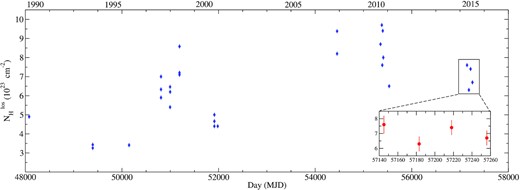
Evolution of the line-of-sight column density (|$N_{\rm H}^{\rm los}$|) in 1023 cm−2 between 1990 and 2015. The blue points are taken from the work of Awaki et al. (1991), Comastri et al. (1998), Risaliti et al. (2002), Matt et al. (2004), Marinucci et al. (2013), and Braito et al. (2013). The inset figure shows the variation of the spectral parameters for this work.
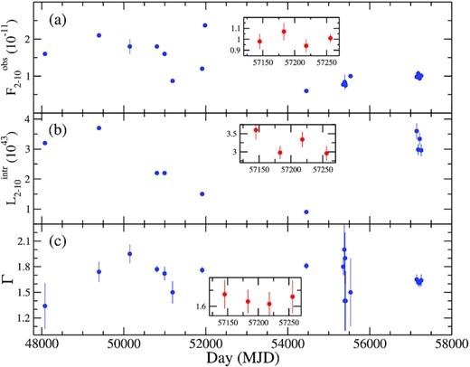
Evolution of (a) the line of sight column density (|$N_{\rm H}^{\rm los}$|) in 1023 cm−2, (b) the 2–10 keV observed flux (|$F^{\rm obs}_{\rm 2-10}$|) in 10−11 erg cm−2 s−1, (c) the 2–10 keV intrinsic luminosity (|$L^{\rm intr}_{\rm 2-10}$|) in 1043 erg s−1, (d) the photon index (Γ) between 1990 and 2015. The blue points are taken from the literature. The inset figures in each panel shows the variation of the spectral parameters from this work.
The line of sight column density was observed to vary in the range of ∼(3–10) × 1023 cm−2 in the past years. In 1990, a Ginga observation revealed a Compton-thin nucleus with NH ∼5 × 1023 cm−2 (Awaki et al. 1991). An ASCA observation, carried out in 1994, also showed a Compton-thin nucleus (NH ∼3 × 1023 cm−2). Risaliti (2002) reported of a Compton-thin absorber (NH ∼5–6 × 1023 cm−2) by studying three BeppoSAX observations performed between 1997 and 1999. A column density of NH ∼4 × 1023 cm−2 was found by XMM–Newton and Chandra observations in 2001 (Matt et al. 2004). Suzaku observed the source in 2007, finding a higher obscuration (NH ∼ 9 × 1023 cm−2; Braito et al. 2013). XMM–Newton and Chandra observation campaign in 2010 reported a variable NH in the range of ∼6.5–9.7 × 1023 cm−2 (Marinucci et al. 2013).
In most of the previous studies, the X-ray spectral analysis was performed with a power law or with the pexrav model. We also performed the spectral analysis using such a phenomenological model, and found that the column density varied in the range ∼(6–8) × 1023 cm−2. Braito et al. (2013) obtained a line-of-sight column density of |$N_{\rm H}^{\rm los}$|∼(6–9) × 1023 cm−2, after applying the MYTD model to the XMM–Newton, Suzaku, and BeppoSAX observations performed between 1997 and 2007. They also estimated the |$N_{\rm H}^{\rm tor}$| ∼(2.4–3.5) × 1023 cm−2. Applying MYTD model to the observations Suzaku in 2007, Tzanavaris et al. (2021) estimated NHlos∼8 ± 0.7 × 1023 cm−2, and NHtor ∼ 2.8 ± 0.4 × 1023 cm−2. In the present work, we found that the global averaged column density of the obscuring material is NHtor∼2.2 ± 0.6 × 1023 cm−2 from the 2015 observations. From this, we can conclude that the global averaged column density of the absorber was nearly constant over decades, which is expected, as the global properties of the circumnuclear material are unlikely to change on the timescale of months. We tabulated the variation of |$N_{\rm H}^{\rm los}$| over the years in Table A6.
In the past 30 yr, the source luminosity was observed to be in the range of |$L_{\rm 2{\!-\!}10}^{\rm intr} \sim (1{\!-\!}4) \times 10^{43}$| erg s−1. In our analysis, we found that the source luminosity is in the range of |$L_{\rm 2{\!-\!}10}^{\rm intr} \sim (3{\!-\!}3.6) \times 10^{43}$| erg s−1. This implies a rather steady accretion on to the SMBH at the centre of NGC 4507. The rms fractional variability of |$\lt 3{{\ \rm per\ cent}}$| in 35 d time-scale also support the steady accretion. At similar luminosity, the rms variability is observed to be in the range of ∼0.1–10 per cent (Fiore et al. 1998). The rms variability is, thus, consistent with other AGNs in similar time-scale (Fiore et al. 1998).
6 SUMMARY
We studied NGC 4507 using NuSTAR observations obtained between 2015 May and 2015 August. Using the phenomenological slab model and several physically motivated torus-based models, we studied the properties of the X-ray emission and of the obscuring gas. We also estimated various properties of the obscuring material, e.g. the line-of-sight column density, the average density of the obscuring material, and its covering factor. From the variability of the absorption, we also provided some refined constraints on the location of the obscuring materials. Our key findings are given below:
We found that the equatorial column density of the torus is Compton-thick (|$N_{\rm H}^{\rm Eq}$| ∼ 2 × 1024 cm−2).
During the period of the observations analysed here, the line-of-sight column density (|$N_{\rm H}^{\rm los}$|) was found to vary in the range of |$N_{\rm H}^{\rm los}$| ∼ 6–9 × 1023 cm−2. The variability of |$N_{\rm H}^{\rm los}$| is observed on time-scales of ≤35 d.
No variability is observed in the primary emission during the observation period.
The source was found to be buried in the obscuring medium, with the torus having a high covering factor Ctor ∼ 0.83–0.85. For the Compton-thick material, the torus covering factor was found to be |$C_{\rm tor}^{\rm T} \sim 0.34{\!-\!}0.37$|, which is in good agreement with average covering factors of the obscuring materials for nearby AGN (e.g. Ricci et al. 2015).
The reprocessing material is found to be located either at the BLR or in the torus.
ACKNOWLEDGEMENTS
We thank the anonymous reviewer for his/her suggestions and comments that helped us to improve the quality of this manuscript. Research at Physical Research Laboratory is supported by the Department of Space, Government of India for this work. AJ and HK acknowledge the support of the grant from the Ministry of Science and Technology of Taiwan with the grand number MOST 110-2811-M-007-500 and MOST 111-2811-M-007-002. HK acknowledge the support of the grant from the Ministry of Science and Technology of Taiwan with the grand number MOST 110-2112-M-007-020. CR acknowledges support from the Fondecyt Iniciacion grant no. 11190831 and ANID BASAL project FB210003. AC and SSH are supported by the Canadian Space Agency and the Natural Sciences and Engineering Research Council of Canada. This research has made use of data and/or software provided by the High Energy Astrophysics Science Archive Research Center (HEASARC), which is a service of the Astrophysics Science Division at NASA/GSFC and the High Energy Astrophysics Division of the Smithsonian Astrophysical Observatory. This work has made use of data obtained from the NuSTAR mission, a projects led by Caltech, funded by NASA and managed by NASA/JPL, and has utilized the nustardas software package, jointly developed by the ASDC, Italy and Caltech, USA.
DATA AVAILABILITY
We used archival data of NuSTAR observatories for this work. All the models used in this work are publicly available. Appropriate links are given in the text.
Footnotes
REFERENCES
APPENDIX A: TABLES
MYTORUS model fitted spectral analysis result for coupled configuration.
| ID | |$N_{\rm H}^{\rm Eq}$| | |$N_{\rm H}^{\rm los}$| | Γ | NPL | it | AS | fScat | χ2/dof |
|---|---|---|---|---|---|---|---|---|
| (1024 cm−2) | (1023 cm−2) | (10−2 ph cm−2 s−1) | (deg) | (10−2) | ||||
| (1) | (2) | (3) | (4) | (5) | (6) | (7) | (8) | (9) |
| N1 | |$2.3^{+0.6}_{-0.9}$| | |$7.5^{+4.2}_{-2.2}$| | |$1.75^{+0.06}_{-0.05}$| | |$3.01^{+0.24}_{-0.17}$| | |$61.8^{+3.7}_{-0.9}$| | |$0.79^{+0.11}_{-0.16}$| | |$1.49^{+0.02}_{-0.03}$| | 664/592 |
| N2 | |$2.0^{+0.7}_{-0.8}$| | |$6.5^{+2.7}_{-1.4}$| | |$1.71^{+0.04}_{-0.05}$| | |$2.15^{+0.12}_{-0.22}$| | ” | |$0.71^{+0.08}_{-0.15}$| | |$1.96^{+0.02}_{-0.03}$| | 620/627 |
| N3 | |$2.5^{+0.7}_{-0.7}$| | |$8.1^{+2.9}_{-1.9}$| | |$1.70^{+0.03}_{-0.05}$| | |$2.89^{+0.12}_{-0.23}$| | ” | |$0.78^{+0.15}_{-0.24}$| | |$1.04^{+0.02}_{-0.03}$| | 634/611 |
| N4 | |$2.0^{+0.6}_{-0.8}$| | |$6.5^{+2.4}_{-1.4}$| | |$1.75^{+0.06}_{-0.05}$| | |$2.09^{+0.18}_{-0.13}$| | ” | |$0.73^{+0.12}_{-0.15}$| | |$1.84^{+0.03}_{-0.08}$| | 584/588 |
Notes. (1) ID of the observation, (2) equatorial hydrogen column density (|$N_{\rm H}^{\rm Eq}$|) in 1024 cm−2, (3) line-of-sight hydrogen column density (|$N_{\rm H}^{\rm los}$|) in 1023 cm−2, (4) photon index (Γ) of the primary emission, (5) power-law normalization (NPL) in 10−2ph cm−2 s−1, (6) inclination angle (i) in degree, (7) relative normalization of the line emission (AS), (9) fraction of scattered primary emission (fScat).
tparameter (6) are tied across the observations.
MYTORUS model fitted spectral analysis result for decoupled configuration.
| ID | |$N_{\rm H}^{\rm los}$| | |$N_{\rm H}^{\rm tor}$| | Γ | NPL | AS | fScat | χ2/dof |
|---|---|---|---|---|---|---|---|
| (1023 cm−2) | (1023 cm−2) | (10−2 ph cm−2 s−1) | (10−2) | ||||
| (1) | (2) | (3) | (4) | (5) | (6) | (7) | (8) |
| N1 | |$8.2^{+1.3}_{-1.3}$| | |$2.2^{+0.6}_{-0.5}$| | |$1.67^{+0.04}_{-0.05}$| | |$3.00^{+0.18}_{-0.31}$| | |$0.71^{+0.03}_{-0.05}$| | |$0.70^{+0.03}_{-0.02}$| | 663/592 |
| N2 | |$7.0^{+1.4}_{-1.3}$| | ” | |$1.65^{+0.08}_{-0.09}$| | |$2.15^{+0.09}_{-0.14}$| | |$0.70^{+0.02}_{-0.04}$| | |$1.40^{+0.01}_{-0.03}$| | 624/625 |
| N3 | |$8.1^{+1.5}_{-1.5}$| | ” | |$1.66^{+0.06}_{-0.06}$| | |$2.69^{+0.05}_{-0.12}$| | |$0.60^{+0.06}_{-0.08}$| | |$0.96^{+0.06}_{-0.02}$| | 633/610 |
| N4 | |$7.1^{+1.3}_{-1.4}$| | ” | |$1.64^{+0.06}_{-0.09}$| | |$1.98^{+0.06}_{-0.07}$| | |$0.71^{+0.05}_{-0.04}$| | |$1.39^{+0.05}_{-0.03}$| | 589/588 |
Notes. (1) ID of the observation, (2) line o of sight hydrogen column density (|$N_{\rm H}^{\rm los}$|) in 1023 cm−2, (3) global averaged hydrogen column density of the obscured materials (|$N_{\rm H}^{\rm tor}$|) in 1023 cm−2, (4) photon index (Γ) of the primary emission, (5) power-law normalization (NPL) in 10−2 ph cm−2 s−1, (6) relative normalization of the line emission (AS), (7) fraction of scattered primary emission (fScat).
tparameter (3) are tied across the observations.
borus02 model fitted spectral analysis result.
| ID | |$N_{\rm H}^{\rm los}$| | t|$N_{\rm H}^{\rm tor}$| | Γ | Ecut | NPL | Ctor | it | tAFe | fScat | χ2/dof |
|---|---|---|---|---|---|---|---|---|---|---|
| (1023) | (1023) | (keV) | (10−2 ph cm−2 s−1) | (degree) | (A⊙) | (10−2) | ||||
| (1) | (2) | (3) | (4) | (5) | (6) | (7) | (8) | (9) | (10) | (11) |
| N1 | |$9.4^{+0.6}_{-0.6}$| | |$2.6^{+0.7}_{-0.6}$| | |$1.48^{+0.06}_{-0.05}$| | |$75^{+29}_{-15}$| | |$1.57^{+0.08}_{-0.11}$| | |$0.58^{+0.10}_{-0.08}$| | |$64.5^{+5.2}_{-6.3}$| | |$0.47^{+0.07}_{-0.06}$| | |$1.02^{+0.11}_{-0.13}$| | 656/592 |
| N2 | |$8.3^{+0.7}_{-0.6}$| | ” | |$1.50^{+0.02}_{-0.04}$| | |$97^{+46}_{-18}$| | |$1.39^{+0.12}_{-0.10}$| | ” | ” | ” | |$1.74^{+0.04}_{-0.03}$| | 620/629 |
| N3 | |$9.8^{+0.6}_{-0.6}$| | ” | |$1.47^{+0.04}_{-0.04}$| | |$91^{+30}_{-23}$| | |$1.51^{+0.16}_{-0.08}$| | ” | ” | ” | |$1.14^{+0.08}_{-0.12}$| | 631/613 |
| N4 | |$8.4^{+0.5}_{-0.5}$| | ” | |$1.46^{+0.04}_{-0.04}$| | |$89^{+43}_{-12}$| | |$1.31^{+0.11}_{-0.13}$| | ” | ” | ” | |$1.61^{+0.09}_{-0.12}$| | 577/592 |
Notes. (1) ID of the observation, (2) line o of sight hydrogen column density (|$N_{\rm H}^{\rm los}$|) in 1023 cm−2, (3) averaged hydrogen column density of the obscured materials. (|$N_{\rm H}^{\rm tor}$|) in 1023 cm−2, (4) cut-off energy (Ecut) in keV, (5) photon index (Γ) of the primary emission, (6) power-law normalization (NPL) in 10−2 ph cm−2 s−1, (7) covering factor the obscured materials, (8) inclination angle (i) in degree, (9) iron abundances (AFe) in solar value (A⊙), (10) fraction of scattered primary emission (fScat).
tparameter (3) and (8) are tied across the observations.
XCLUMPY model fitted spectral analysis result.
| ID | t|$N_{\rm H}^{\rm Eq}$| | |$N_{\rm H}^{\rm los}$| | Γ | NPL | σtor | it | AL | fScat | χ2/dof |
|---|---|---|---|---|---|---|---|---|---|
| (1024) | (1023) | (10−2ph cm−2 s−1) | (degree) | (degree) | (10−2) | ||||
| (1) | (2) | (3) | (4) | (5) | (6) | (7) | (8) | (9) | (10) |
| N1 | |$2.1^{+0.6}_{-0.3}$| | |$8.1^{+2.4}_{-1.5}$| | |$1.67^{+0.06}_{-0.12}$| | |$1.78^{+0.10}_{-0.18}$| | |$26.3^{+8.4}_{-5.3}$| | |$64.1^{+7.4}_{-4.9}$| | |$0.78^{+0.10}_{-0.08}$| | |$1.78^{+0.42}_{-0.65}$| | 652/595 |
| N2 | ” | |$7.0^{+1.6}_{-1.1}$| | |$1.66^{+0.12}_{-0.07}$| | |$0.88^{+0.14}_{-0.18}$| | |$24.9^{+4.6}_{-7.1}$| | ” | |$0.84^{+0.07}_{-0.11}$| | |$4.30^{+0.53}_{-0.86}$| | 616/628 |
| N3 | ” | |$8.2^{+1.6}_{-2.3}$| | |$1.63^{+0.09}_{-0.12}$| | |$1.63^{+0.18}_{-0.25}$| | |$25.7^{+5.2}_{-5.8}$| | ” | |$0.76^{+0.08}_{-0.11}$| | |$2.12^{+0.34}_{-0.29}$| | 629/613 |
| N4 | ” | |$7.1^{+1.5}_{-2.2}$| | |$1.59^{+0.12}_{-0.15}$| | |$1.31^{+0.18}_{-0.12}$| | |$25.2^{+4.6}_{-4.9}$| | ” | |$0.88^{+0.10}_{-0.09}$| | |$2.57^{+0.27}_{-0.38}$| | 579/590 |
Notes. (1) ID of the observation, (2) equatorial hydrogen column density (|$N_{\rm H}^{\rm Eq}$|) in 1024 cm−2, (3) line of sight hydrogen column density (|$N_{\rm H}^{\rm los}$|) in 1023 cm−2, (4) photon index (Γ) of the primary emission, (5) power-law normalization (NPL) in 10−2ph cm−2 s−1, (6) torus angular width (σtor) in degrees, (7) inclination angle (i) in degree, (8) relative normalization of the line emission (AL), (9) fraction of scattered primary emission (fScat).
tparameter (2) and (7) are tied across the observations.
rxtorus model fitted spectral analysis result.
| ID | t|$N_{\rm H}^{\rm Eq}$| | |$N_{\rm H}^{\rm los}$| | Γ | it | r/R | NPL | Arpcr | fScat | χ2/dof |
|---|---|---|---|---|---|---|---|---|---|
| (1024) | (1023) | (degree) | (10−2ph cm−2 s−1) | (10−2) | |||||
| (1) | (2) | (3) | (4) | (5) | (6) | (7) | (8) | (9) | (10) |
| N1 | |$2.1^{+0.6}_{-0.5}$| | |$6.9^{+2.4}_{-1.6}$| | |$1.63^{+0.07}_{-0.06}$| | |$66.7^{+4.5}_{-7.2}$| | |$0.42^{+0.07}_{-0.09}$| | |$1.75^{+0.08}_{-0.07}$| | |$1.04^{+0.15}_{-0.11}$| | |$1.58^{+0.45}_{-0.75}$| | 652/596 |
| N2 | ” | |$6.0^{+0.9}_{-1.1}$| | |$1.58^{+0.10}_{-0.08}$| | ” | |$0.41^{+0.09}_{-0.07}$| | |$1.46^{+0.12}_{-0.16}$| | |$1.03^{+0.14}_{-0.19}$| | |$2.14^{+0.09}_{-0.12}$| | 615/629 |
| N3 | ” | |$7.0^{+1.6}_{-1.8}$| | |$1.60^{+0.06}_{-0.07}$| | ” | |$0.42^{+0.08}_{-0.07}$| | |$1.70^{+0.08}_{-0.12}$| | |$0.97^{+0.06}_{-0.12}$| | |$1.74^{+0.08}_{-0.11}$| | 625/615 |
| N4 | ” | |$6.1^{+1.5}_{-2.1}$| | |$1.57^{+0.06}_{-0.07}$| | ” | |$0.41^{+0.08}_{-0.08}$| | |$1.36^{+0.10}_{-0.11}$| | |$1.06^{+0.16}_{-0.21}$| | |$2.11^{+0.18}_{-0.22}$| | 578/592 |
Notes. (1) ID of the observation, (2) equatorial hydrogen column density (|$N_{\rm H}^{\rm Eq}$|) in 1024 cm−2, (3) line of sight hydrogen column density (|$N_{\rm H}^{\rm los}$|) in 1023 cm−2, (4) photon index (Γ) of the primary emission, (5) inclination angle (i) in degree, (6) torus covering factor (r/R), (7) power-law normalization (NPL) in 10−2ph cm−2 s−1, (8) relative normalization of the reprocessed emission (Arpcr), (9) fraction of scattered primary emission (fScat).
tparameter (2) and (7) are tied across the observations. Line-of-sight hydrogen column density is calculated using equation (3).
Variation of line-of-sight column density (|$N_{\rm H}^{\rm los}$|).
| Date | |$N_{\rm H}^{\rm los}$| | |$F_{2-10~{\rm keV}}^{\rm obs}$| | Observatories | Ref. |
|---|---|---|---|---|
| (YYYY-MM-DD) | (1023 cm−2) | (10−11 erg cm−2 s−1) | ||
| (1) | (2) | (3) | (4) | (5) |
| 1990-07-07 | 4.9 ± 0.7 | 1.6a | Ginga | Awaki et al. (1991) |
| 1994-02-12 | 3.26 ± 0.7 | 2.1a | ASCA | Comastri et al. (1998) |
| 1996-03-05 | 3.41 ± 0.11 | 1.8 ± 0.2 | RXTE | Guainazzi et al. (1997) |
| 1997-12-26 | 7.00 ± 0.45 | 1.8a | BeppoSAX | Braito et al. (2013) |
| 1998-07-02 | 6.20 ± 0.50 | 1.6a | BeppoSAX | Braito et al. (2013) |
| 1999-01-13 | 6.40 ± 0.95 | 0.87a | BeppoSAX | Risaliti (2002) |
| 2001-01-04 | 5.0 ± 0.25 | 1.2a | XMM–Newton | Braito et al. (2013) |
| 2001-03-15 | 4.0a | 2.37a | Chandra | Matt et al. (2004) |
| 2007-12-20 | 8.2 ± 0.6 | 0.6a | Suzaku | Braito et al. (2013) |
| 2010-06-24 | 8.7 ± 0.7 | 7.7 ± 0.3 | XMM–Newton | Marinucci et al. (2013) |
| 2010-07-03 | 9.7 ± 0.9 | 8.0 ± 0.3 | XMM–Newton | Marinucci et al. (2013) |
| 2010-07-13 | 7.6 ± 1.1 | 8.4 ± 0.2 | XMM–Newton | Marinucci et al. (2013) |
| 2010-07-23 | 9.4 ± 1.1 | 8.0 ± 0.3 | XMM–Newton | Marinucci et al. (2013) |
| 2010-08-03 | 8.0 ± 0.7 | 7.5 ± 0.7 | XMM–Newton | Marinucci et al. (2013) |
| 2010-12-02 | 6.5 ± 0.7 | 10.0 ± 0.4 | Chandra | Marinucci et al. (2013) |
| 2015-05-03 | 0.79 ± 0.03 | 0.98 ± 0.07 | NuSTAR | This work |
| 2015-06-10 | 0.69 ± 0.02 | 1.07 ± 0.08 | NuSTAR | This work |
| 2015-07-15 | 0.78 ± 0.03 | 0.94 ± 0.06 | NuSTAR | This work |
| 2015-08-22 | 0.73 ± 0.02 | 1.01 ± 0.04 | NuSTAR | This work |
aNo error is quoted.
APPENDIX B: SPECTRA
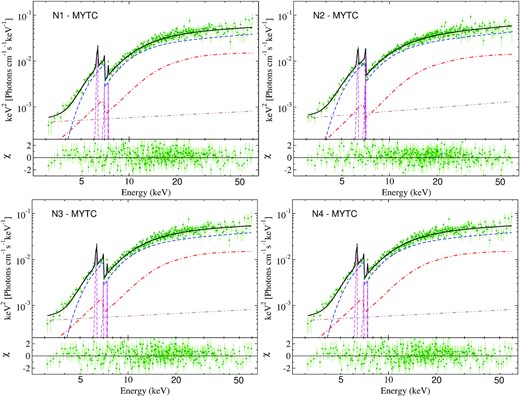
Unfolded spectra fitted with MYTC model for observation N1 (top left), N2 (top right), N3 (bottom left), and N4 (bottom right). Upper panel: Green points represent the data. The black, blue, red, magenta, and brown lines represent the total emission, primary emission, reprocessed emission, line emission (Fe Kα, Fe Kβ, and Ni K α), and scattered primary emission. Bottom panel: Corresponding residual.
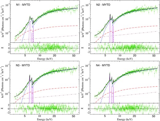
Unfolded spectra fitted with MYTD model for observation N1 (top left), N2 (top right), N3 (bottom left) and N4 (bottom right). Upper panel: Green points represent the data. The black, blue, red, magenta and brown lines represent the total emission, primary emission, reprocessed emission, line emission (Fe Kα, Fe Kβ and Ni K α), and scattered primary emission. Bottom panel: Corresponding residual.
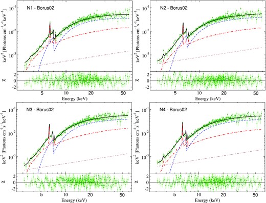
Unfolded spectra fitted with borus02 model for observation N1 (top left), N2 (top right), N3 (bottom left), and N4 (bottom right). Upper panel: Green points represent the data. The black, blue, red, magenta and brown lines represent the total emission, primary emission, reprocessed emission, line emission (Fe Kα, Fe Kβ, and Ni Kα), and scattered primary emission. Bottom panel: Corresponding residual.
Unfolded spectra fitted with xclumpy model for observation N1 (top left), N2 (top right), N3 (bottom left), and N4 (bottom right). Upper panel: Green points represent the data. The black, blue, red, magenta, and brown lines represent the total emission, primary emission, reprocessed emission, line emission (Fe Kα, Fe Kβ and Ni Kα), and scattered primary emission. Bottom panel: Corresponding residual.
Unfolded spectra fitted with RXTorus model for observation N1 (top left), N2 (top right), N3 (bottom left), and N4 (bottom right). Upper panel: Green points represent the data. The black, blue, red, magenta and brown lines represent the total emission, primary emission, reprocessed emission, line emission (Fe Kα, Fe Kβ, and Ni Kα), and scattered primary emission. Bottom panel: Corresponding residual.
APPENDIX C: CONTOUR
Confidence contour between the photon index (Γ) and equatorial column density (NH) in 1022 cm−2, fitted with the MYTC model. The red, blue, magenta, and orange lines represent the observation from N1, N2, N3, and N4, respectively. The solid and dashed lines represent the contour at 1σ and 2σ levels, respectively.
Confidence contour between the line of sight column density (NH) and averaged torus column density in 1022 cm−2, fitted with the MYTD model. The red, blue, magenta, and orange lines represent the observation from N1, N2, N3, and N4, respectively. The solid and dashed lines represent the contour at 1σ and 2σ levels, respectively.
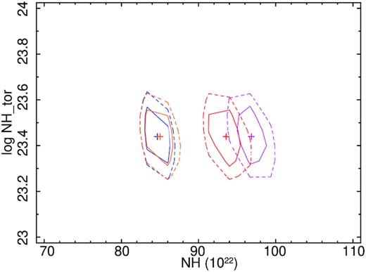
Confidence contour between the line of sight column density (NH) and averaged torus column density in 1022 cm−2, fitted with the borus02 model. The red, blue, magenta, and orange lines represent the observation from N1, N2, N3, and N4, respectively. The solid and dashed lines represent the contour at 1σ and 2σ levels, respectively.
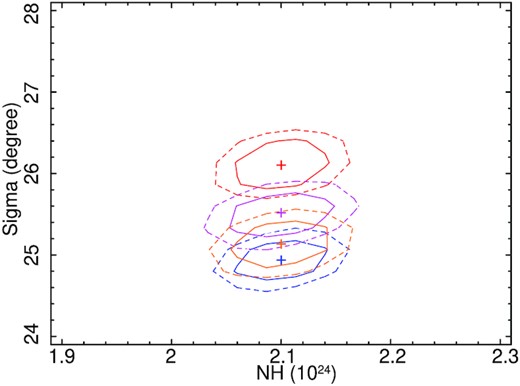
Confidence contour between the equatorial column density (|$N_{\rm H}^{\rm Eq}$|) and torus angular width, fitted with the xclumpy model. The red, blue, magenta, and orange lines represent the observation from N1, N2, N3, and N4, respectively. The solid and dashed lines represent the contour at 1σ and 2σ level, respectively.
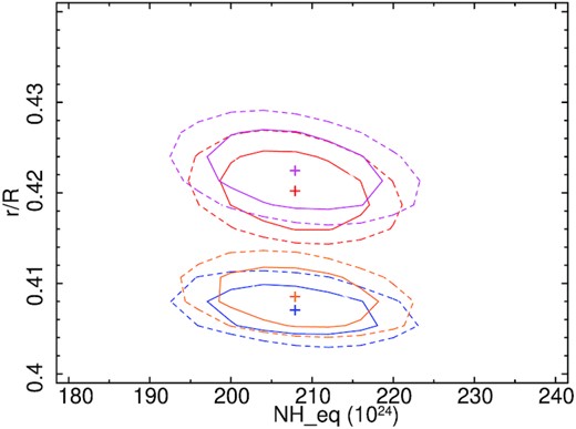
Confidence contour between the equatorial column density (|$N_{\rm H}^{\rm Eq}$|) and covering factor, fitted with the RXTorus model. The red, blue, magenta, and orange lines represent the observation from N1, N2, N3, and N4, respectively. The solid and dashed lines represent the contour at 1σ and 2σ levels, respectively.
