


ABSTRACT
The self-organized criticality (SOC) is a universal theory to explain the ubiquitous power-law size distributions of astrophysical instabilities such as solar eruptions. One way to understand the dynamical processes of an SOC system is through cellular automaton (CA) simulations. Here, we develop a three-dimensional solar CA model that assumes a twisted magnetic flux rope (MFR), in which the avalanche takes place when a local magnetic vector potential exceeds a Gaussian distributed instability criterion, triggered by a global and space-dependent energy driving mechanism. To avoid non-physical released energies, an energy screening mechanism is applied to calculate the avalanche energies of each time-step. Our results show that the statistics of the CA simulated flaring events are comparable to the frequency distributions of observed solar flares originating from an individual active region. Due to the fact of the universality of MFRs, the CA model can be applied to many other astrophysical SOC systems.
1 INTRODUCTION
The concept of self-organized criticality (SOC) dated from the landmark paper ‘Self-organized criticality: An explanation of 1/f noise’ (Bak, Tang & Wiesenfeld 1987). The SOC describes a non-linear dynamical system that is driven towards a critical state independent of external parameters, and then produces intermittent avalanches with power-law frequency distributions (Aschwanden 2012; Pruessner 2012; Aschwanden et al. 2016). It is then widely applied to explain the ubiquitous power-law size distributions of astrophysical phenomena, as done by some recent studies of solar and stellar flares (Li et al. 2018; Aschwanden 2019; Lei et al. 2020; Tu et al. 2021), gamma-ray bursts (Wang & Dai 2013; Harko, Mocanu & Stroia 2015; Yi et al. 2016), fast radio bursts (Wang & Yu 2017), and magnetar bursts (Göǧüş et al. 2000; Cheng, Zhang & Wang 2020; Lin et al. 2020).
One way to explore the spatiotemporal evolution of an SOC system is through cellular automaton (CA) simulations. The original CA model is the so-called sand pile model (Bak et al. 1987; Bak, Tang & Wiesenfeld 1988), which successfully reproduced the power-law size distributions of sand-pile avalanches and explained the ubiquitous flicker noise. The first solar CA model was proposed by Lu & Hamilton (1991), who conceived the solar coronal magnetic field is distributed in a grid. An avalanche takes place when a local magnetic field gradient exceeds a critical value and leads to magnetic relaxation, similar to the critical discontinuity angle condition leading to the magnetic reconnection proposed by Parker (1988). The Lu & Hamilton model found the approximately power-law distributions of solar flare duration, peak fluxes, and released energies. In the past two decades, some physics-based CA models have been proposed by using various driving mechanisms, stability criterions, and redistribution rules (Vassiliadis et al. 1998; Isliker, Anastasiadis & Vlahos 2000; Charbonneau et al. 2001; Morales & Charbonneau 2008; Strugarek et al. 2014; Farhang, Safari & Wheatland 2018; Farhang, Wheatland & Safari 2019), to simulate the occurrence of solar magnetic energy releases.
In the present study, we extend the two-dimensional (2D) solar CA models of Strugarek et al. (2014) and Farhang et al. (2018) to a new version of three-dimensional (3D) model that assumes a twisted magnetic flux rope (MFR), where an avalanche takes place when a local magnetic vector potential exceeds a Gaussian distributed instability criterion. The avalanches are then triggered by a global and space-dependent energy driving mechanism that is comparable to the twisting forms of real magnetic flux ropes (Guo et al. 2017; Wang et al. 2018). To calculate the released energies for each time-step, an energy screening mechanism is applied to avoid non-physical avalanche energies.
We introduce, in Section 2, how the avalanche model is constructed, including the 3D lattice of an MFR, driving mechanism, stability criterion, and redistribution rule. In Section 3, the simulated avalanches are compared to the frequency distributions of flaring events originating from an individual solar active region (AR). We conclude in Section 4 by summarizing the results and discussing further applications of the avalanche model.
2 THE AVALANCHE MODEL FOR SOLAR FLARES
Solar flares, with energies ranging from 1029 to 1032 erg (Crosby, Aschwanden & Dennis 1993; Aschwanden et al. 2000; Shibata & Magara 2011), are one of the most eruptive phenomena on the Sun powered by magnetic energy release. Recent studies have shown that MFRs probably play the key role in producing solar eruptions, namely flares and coronal mass ejections (Chen 2011; Zhang, Cheng & Ding 2012; Cheng, Guo & Ding 2017; Xing, Cheng & Ding 2020). It was found that the MFRs exist in ∼89 per cent of filament eruptions (Ouyang et al. 2017). Therefore, it might be more appropriate to perform the solar CA simulations in such flux-rope-topology SOC systems.
2.1 Lattice construction
The sketch map of our solar CA model is shown in Fig. 1. The left-hand panel displays an MFR constructed by using the analytical Titov–Démoulin-modified (TDm) model (Titov et al. 2014, 2018). Here, the TDm method is applied only to produce a flux-rope-like structure that has a circular cross-section and a certain twist around the axis. To be mentioned that the MFR may possess increasing, uniform, and decreasing numbers of twists from its centre to the boundary based on the magnetic field extrapolations and real observations (Guo et al. 2017; Wang et al. 2018). It indicates the magnetic energy accumulation may take place uniformly or non-uniformly in an MFR, and leads us to propose the three cases of driving mechanisms described in the following text. The middle panel depicts the straightened and latticed MFR composed of 30 × 30 × 30 lattice nodes. Each node is designated a magnetic vector potential |$A_{i,j,k}\hat{z}$|, hence the solenoidal constraint ∇ · B = 0 is satisfied automatically.
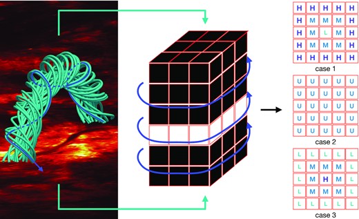
Sketch map of the 3D solar CA model. The left-hand panel shows a magnetic flux rope constructed by using the TDm model. The middle panel shows the latticed flux rope composed of 30 × 30 × 30 nodes. The right-hand panel describes three kinds of driving mechanisms leading to avalanches.
2.2 Driving mechanism
2.3 Stability criterion
2.4 Redistribution rules
We then apply an energy screening mechanism to calculate the energy release of each avalanche. We examine the released energy of every node for each time-step. Only the nodes leading to positive released energies are used to calculate the released energy of present step, while those with negative released energies keep unstable till to the next step. This avoids non-physical avalanche energies and ensures the maximum energy released in each avalanche.
2.5 Avalanche statistics
We have run the solar CA simulations described in the preceding text. Fig. 2 shows the J|$z$| distributions at the middle cross-sections of the flux ropes corresponding to the three cases of driving mechanisms. The J|$z$| is integrated through all iterations in statistically equilibrated states, in other words, non-avalanching iterations. It can be found that the J|$z$| is not uniformly distributed, but peaked at the edge for the case 1 and at the centre for the case 3. This is due to the fact of larger twist or energy input at the boundary for case 1 and at the centre for case 3, that leads to larger J|$z$| in these nodes. It is also found that the J|$z$| distribution departs from axisymmetry about the lattice centre, especially for the case 2. This is due to the anisotropic redistribution rules described in equation (6).
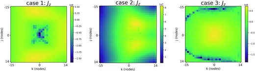
The J|$z$| distributions at the middle cross-sections for the three cases of driving mechanisms.
Fig. 3 shows the evolution of the lattice energy (upper panel) and the released energy (bottom panel) for the case 2 – uniformly distributed driving rate. It can be seen that the lattice energy is continuously increasing, especially in the first ∼1 × 10⁶ iterations, similar to the deposition of free magnetic energy in a developing solar AR. Each spike in the bottom panel of Fig. 3 represents a single process of energy release, and an avalanching event may consist of many spikes as shown by the two embedded panels. Here an avalanching event is determined when the number of avalanching nodes, rather than the unstable nodes, returns to zero. It means that the unstable nodes may not release energy according to the energy screening mechanism introduced previously. These unstable nodes may contribute to an avalanching event at next iteration. There are totally 5214 avalanching events recorded during the whole 5 × 10⁶ iterations.
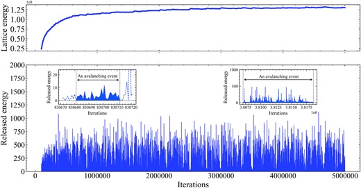
Time series of the lattice energy (upper panel) and the released energy (bottom panel) of simulated avalanches during all the 5 × 10⁶ iterations.
One interesting result of the avalanche statistics is that the first 1 × 10⁶ iterations produce 4619 avalanching events (hereafter as group 1), while the last 4 × 10⁶ iterations produce only 595 events (hereafter as group 2). It is probably due to the fact that the events of group 2 have much longer duration and larger released energies comparing to the group 1. The two embedded panels in Fig. 3 represent the two typical avalanching events of group 1 and group 2, respectively. We then plot Fig. 4 that shows the event number distributions of the avalanching duration, maximum energies (peak intensities), and released energies for the two groups. It is found that the avalanching duration and released energies of group 2 tend to distributed at relatively larger values comparing to the group 1. The possible reason is that the energy deposition in the 3D lattice is continuously increasing, more lattice nodes are driven to quasi-critical states, therefore leading to larger avalanches.
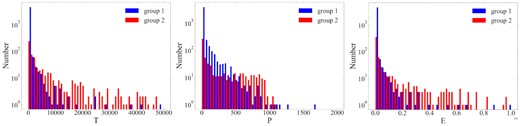
Event number distributions of the avalanching duration, peak intensities, and released energies for the two groups of avalanching events described in the text.
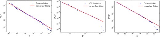
Frequency distributions of the CA simulated avalanching duration, peak intensities, and released energies. The avalanche statistics are derived from all the 5 × 10⁶ iterations. The fitting is carried out with power-law PDFs by using the MCMC method.
Fitting parameters of the frequency distributions for the observational and simulated flaring events. The avalanche statistics are derived from all the 5 × 10⁶ iterations.
| αT | αP | αE | |
|---|---|---|---|
| AR12673 | |${1.44}^{+0.26}_{-0.27}$| | |${1.25}^{+0.13}_{-0.14}$| | |${1.12}^{+0.07}_{-0.08}$| |
| Case 1 | |${1.56}^{+0.02}_{-0.02}$| | |${2.22}^{+0.09}_{-0.09}$| | |${1.34}^{+0.02}_{-0.02}$| |
| Case 2 | |${1.35}^{+0.01}_{-0.01}$| | |${1.29}^{+0.02}_{-0.02}$| | |${1.18}^{+0.01}_{-0.01}$| |
| Case 3 | |${1.47}^{+0.02}_{-0.02}$| | |${2.26}^{+0.05}_{-0.05}$| | |${1.56}^{+0.04}_{-0.04}$| |
3 SOLAR FLARES PRODUCED BY AR12673
We investigate the flare occurrence in an individual solar AR, rather than from the whole solar disc. It approaches the idea of avalanches in a single MFR, and avoids the statistical bias arising from the irrelevant flaring events produced in other ARs (Wheatland 2000; Lei et al. 2020). The AR12673 was one of the most productive ARs, and was observed by the Solar Dynamics Observatory (SDO; Pesnell, Thompson & Chamberlin 2012) since its emergence to disappearance behind the solar limb.
We examine the light curve of AR12673 by using the high-cadence (∼12 s) observations from the Atmospheric Imaging Assembly (AIA, Lemen et al. 2012) onboard the SDO. Fig. 6 shows the temporal evolution of AR12673 in the SDO/AIA 94 Å passband. This passband corresponds to Fe 18 ions at temperatures of ∼6 × 10⁶ K, featuring very hot flaring regions rather than the quiet Sun, and leading flares stand out clearly in the image (Verbeeck et al. 2019). The upper panels of Fig. 6 display a snapshot of the full-disc image at 07:56 ut, 2017 September 4 and the zoomed-in image of AR12673, respectively. The bottom panel displays the light curve of AR12673 from its emergence on 2017 September 1 to its disappearance behind the west solar limb on 2017 September 10. The intensity is normalized by exposure time and pixel number. The red line indicates the flaring events identified by the following criteria: (1) the peak flux of a spike exceeds 40 |${{\ \rm per\ cent}}$| of the local background, similar to the criterion of GOES soft X-ray flare determination; (2) the onset time of a flare is determined when the flux exceeds 10 |${{\ \rm per\ cent}}$| of the local background; and (3) the end time is determined to be when the flux falls back to onset value or at the minimum value before another flare spike. It allows us to identify 78 solar flares. The inset in the bottom panel of Fig. 6 depicts a case of verified flare and the parameters of flare duration, peak flux, and integral energy.
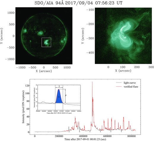
Upper panel: A snapshot of the full-disc image and the zoomed-in AR12673 observed with the SDO/AIA 94 Å passband. Bottom panel: The light curve of AR12673 from its emergence on 2017 September 1 to its disappearance behind the west solar limb on 2017 September 10. An example flare and its duration, peak intensity, and integral energy are illustrated in the inset panel.
Applying also the MCMC method, we present, in Fig. 7, the fitting results of frequency distributions for the solar flares produced by AR12673. The error bars are calculated as |$\sqrt{N_i \Delta x_i} / \Delta x_i$|, where Ni is the number of the ith bin and Δxi is the bin width. The power-law indices are derived to be αT = 1.45 ± 0.05 for the flare duration, αP = 1.25 ± 0.04 for the peak fluxes, and αE = 1.14 ± 0.04 for the integral energies. Table 1 compares the fitting parameters of the frequency distributions for the observational and simulated flaring events.
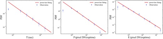
Frequency distributions of the observed flare duration, peak intensity, and integral fluence. The fitting is carried out with power-law PDFs by using the MCMC method.
4 SUMMARY AND DISCUSSION
We introduce a 3D lattice-based CA model to simulate the flaring events of a twisted MFR in the state of SOC. The lattice nodes are distributed with magnetic vector potentials that automatically satisfy the divergence free condition of magnetic field. A global and space-dependent driving mechanism is applied to trigger the avalanche or magnetic relaxation that leads the system to a state of minimum possible energy. The simulated flaring events are statistically characterized as power-law frequency distributions. To compare with real observations, we investigate the flare occurrence rate in an individual solar AR. It is found that, as shown in Table 1, the statistical results of observed solar flares are comparable to the frequency distributions of CA simulated flaring events, especially in case 2 – uniformly distributed driving rate.
It should be mentioned that the present CA model can produce power-law distribution of avalanching events in its early phase, due to fact that most of the avalanching events take place in the first simulating 1 × 10⁶ iterations. More relatively larger avalanches are produced in its later phase. These are different from the 2D models of Strugarek et al. (2014) and Farhang et al. (2018). In the first model, the initial condition of magnetic vector potentials were set to be zero, it therefore needs a certain number of steps to reach the SOC states or the so-called statistically stationary phase. In the second model, the initial magnetic vector potentials were set to be uniformly random numbers as done in present study, the SOC states were reached very quickly, and no ‘early transient phase’ was identified. The possible reason of existing an early phase in present model is that the energy deposition of 3D lattice nodes is continuously increasing until to a system-wide saturated phase with more nodes in quasi-critical states, then producing longer and larger avalanches. This continuously increasing lattice energy is similar to the real observations that the free magnetic energy in a developing solar AR, and larger solar eruptions prefer to occur in an AR with larger free magnetic energies.
Another point should be mentioned that the present 3D model generates relatively smaller power-law indices compared to the original solar CA model (Lu & Hamilton 1991) and the model of Farhang et al. (2018), but comparable to the model of Strugarek et al. (2014). Two reasons probably lead to the smaller exponents. At first, the imposed energy screening mechanism may make the unstable nodes keeping unstable, leading to larger avalanches at next iterations. And then, the principle of minimum energy has also a priority to produce larger avalanches.
As a summary, the MFRs are ubiquitous structures in the Universe, e.g. the magnetic clouds in interplanetary space, the Birkeland currents in magnetosphere, the filaments in the interstellar medium, the flux tubes around magnetar, and the relativistic jets from black holes. Different kinds of MFRs in a state of SOC might produce avalanches via different energy driving mechanisms described in the preceding text. Therefore, the present CA model can be further developed and applied to many other astrophysical eruptions, such as geomagnetic storms, stellar flares, gamma-ray bursts, and magnetar bursts.
ACKNOWLEDGEMENTS
This work was supported by the National Key Research and Development Program of China (grant number 2020YFC2201200), the National Natural Science Foundation of China (grant numbers 11673012, 11533005, 11961131002, and U1831207), and the ‘Integration of Space- and Ground-based Instruments’ project of the China National Space Administration (CNSA). The authors thank the SDO/AIA team for providing the observational data.
DATA AVAILABILITY
The data underlying this article will be shared on reasonable request to the corresponding author.
