


ABSTRACT
Blazars optical emission is generally dominated by relativistic jets, although the host galaxy, accretion disc, and broad-line region (BLR) may also contribute significantly. Disentangling their contributions has been challenging for years due to the dominance of the jet. To quantify the contributions to the spectral variability, we use the statistical technique for dimensionality reduction non-negative matrix factorization on a spectroscopic data set of 26 γ-ray blazars. This technique allows to model large numbers of spectra in terms of a reduced number of components. We use a priori knowledge to obtain components associated with meaningful physical processes. The sources are classified according to their optical spectrum as host-galaxy dominated BL Lac objects (BL Lacs), BL Lacs, or flat spectrum radio quasars (FSRQs). Host-galaxy sources show less variability, as expected, and bluer-when-brighter (BWB) trends, as the other BL Lacs. For FSRQs, more complicated colour-flux behaviours are observed: redder-when-brighter for low states saturating above a certain level and, in some cases, turning to BWB. We are able to reproduce the variability observed during 10 yr using only two to four components, depending on the type. The simplest scenario corresponds to host-galaxy blazars, whose spectra are reconstructed using the stellar population and a power law (PL) for the jet. BL Lac spectra are reproduced using from two to four PLs. Different components can be associated with acceleration/cooling processes taking place in the jet. The reconstruction of FSRQs also incorporates a QSO-like component to account for the BLR, plus a very steep PL, associated with the accretion disc.
1 INTRODUCTION
Blazars are a subclass of active galactic nuclei (AGNs) whose relativistic jets are closely aligned with the line of vision, characterized by a strong flux variability. Their emission can extend from radio wavelengths up to very-high-energy (VHE) γ-rays with energies of a few TeVs. The spectral energy distribution (SED) of these sources shows a double bump structure (e.g. Abdo et al. 2010a). The first bump is caused by the synchrotron emission of relativistic electrons coming from the jet (Ghisellini et al. 2010). The second one is commonly explained with a leptonic scenario via inverse-Compton (IC) scattering of the synchrotron photons of the same electron population (synchrotron self-Compton, SSC; Maraschi, Ghisellini & Celotti 1992), and/or IC of seed photons from outside the jet (external Compton, EC, see e.g. Dermer & Schlickeiser 1994). Alternatively, models based on hadronic processes have been proposed to explain and reproduce the high-energy (HE) bump of these objects (e.g. Cerruti et al. 2015). Blazars can be subdivided in two groups (Urry & Padovani 1995): BL Lac objects and flat spectrum radio quasars (FSRQs). Both classes can be distinguished by their optical spectra. BL Lacs show an optical spectrum with (almost) no features, whereas FSRQs have narrow and broad lines in their spectrum with a rest-frame equivalent width EW >5 Å (e.g. Stickel et al. 1991; Stocke et al. 1991). Moreover, they also differ in the frequency ν of the SED peaks and their intensity ratio (Compton dominance; Finke 2013). Furthermore, they can also be classified according to the frequency of the synchrotron peak of the SED as low-, intermediate-, and high-synchrotron peaked blazars (LSPs, ISPs and HSPs, respectively). LSPs display a synchrotron peak located at νsync < 1014 Hz. ISPs show their synchrotron peak between frequencies of 1014 < νsync < 1015 Hz. Finally, HSPs have a synchrotron peak frequency νsync > 1015 Hz.
Variability in these sources has been detected in a wide range of time-scales (see e.g. Fan 2005): in scales as short as a few minutes or several hours (intraday variability, for instance, Vovk & Babić 2015), longer time-scale variations on the order of days to weeks (short-term variability; e.g. Abdo et al. 2010b), and variations in scales of months to years (long-term variability; e.g. Sandrinelli, Covino & Treves 2014). Variability has a crucial importance in the understanding of these violent sources, since it has been interpreted within several scenarios, depending on the nature and time-scale of the variation. For instance, intraday variability has been explained in terms of flare-like events or phenomena such as the lighthouse effect presented by Camenzind & Krockenberger (1992). Another interpretation involves the combination of chromatic variations linked to substructures in the jet, shocks propagating in turbulent plasma, and stochastic processes related to the injection and acceleration of particles, and/or changes of the Doppler factor most likely due to variations of the viewing angle (Raiteri et al. 2021a,b). Moreover, short-term variability may be caused by instabilities or variations in the accretion rate (Mangalam & Wiita 1993). Long-term variations in blazars have been interpreted with several models, e.g. a binary black hole system with a precession period of the secondary black hole around the primary (Lehto & Valtonen 1996), helical jets (Raiteri et al. 2010), shocks (Marscher & Gear 1985) or changes in the viewing angle (Raiteri et al. 2017). These long-term variations have been detected in the past showing periodic patterns (see e.g. Ackermann et al. 2015; Sandrinelli et al. 2018; Fan et al. 2018a; Covino, Sandrinelli & Treves 2019; Otero-Santos et al. 2020; Peñil et al. 2020; Zhang et al. 2020). These flux variations are frequently associated with spectral variability of the source (see e.g. Bonning et al. 2012; Zhang et al. 2015; Isler et al. 2017; Li et al. 2018).
The synchrotron emission coming from the relativistic jets is the main contribution to their optical emission (Blandford & Rees 1978). Nevertheless, other regions [e.g. host galaxy, broad-line region (BLR) in FSRQs, or accretion disc] may contribute significantly to the emission (e.g. Massaro et al. 2015; Raiteri et al. 2019). In such cases, all these components must be taken into account when studying the variability of the source. However, disentangling these contributions to the emission of blazars has been challenging due to the high dominance of the emission from the jet.
Understanding the origin of this variability in blazars is crucial to comprehend the processes taking place in the most extreme Universe. Several previous studies have tried to explain and reproduce the variability in AGNs taking into account the different contributions. For this purpose, statistical tools for dimensionality reduction have been used, such as the principal component analysis (PCA; see Pearson 1901; Hotelling 1933; Ivezić et al. 2014) or the non-negative matrix factorization (NMF, see Paatero & Tapper 1994; Ivezić et al. 2014). These techniques allow the reconstruction of a large data set by making use of a reduced number of components. They have been applied before to other types of AGNs, in which the jet does not outshine the other contributions, due to a larger viewing angle (Hurley et al. 2014; Parker et al. 2015; Zhu 2016; Gallant, Gallo & Parker 2018). However, the powerful jets of blazars make the application of such technique challenging. Nevertheless, understanding the impact of other physical regions such as the accretion disc or the BLR to the global variability observed in blazars is a matter of great importance to comprehend the processes taking place in the environment of these extreme sources. For this purpose, the combination of statistical tools such as the NMF together with some physical assumptions based on our knowledge of the different components, can help to shed light to the overall emission of blazars.
This work is focused on the characterization of the overall optical variability of a blazar sample based on the minimum number of spectral components. The global variability of the sources and the contribution of each component to the overall flux variation are studied. For this purpose, the NMF is used to decompose the optical spectra of each source and identify the different components contributing to the emission. A first approach of applying the NMF to model and reproduce the variability observed in blazars was performed in the past by Acosta-Pulido et al. (2017). For this analysis, we make use of the observations performed by the Steward Observatory in Arizona, as a support program for the Fermi satellite observations of bright γ-ray blazars. Photometric and spectropolarimetric data of a large sample of blazars are available, with a time coverage of ∼10 yr. This paper is structured as follows: In Sections 2 and 3, we introduce the data set used in the analysis, the data reduction and the variability observed in the data sample; in Section 4, the analysis tools and the methodology followed for this work are presented; in Sections 5 and 6, we present the results of the analysis and the physical interpretation and implications of these results. The conclusions and final remarks of this work are summarized in Section 7. Finally, a detailed discussion on some sources of interest is included in Appendix A.
2 OBSERVATIONS AND DATA REDUCTION
We have analysed the optical spectral data taken by the Steward Observatory program in support of the Fermi-LAT γ-ray observations1 of a sample of blazars. The Steward Observatory has monitored a sample of 80 blazars from 2008 October until 2018 July (Smith et al. 2009). We have selected those sources with more than 15 spectra available. This selection criteria led us to a final data sample of 26 sources, listed in Table 1. A total of 11 sources have been classified as BL Lac objects and 12 are FSRQs. The three remaining ones are BL Lac objects whose optical spectra are dominated by the stellar emission from the host galaxy (hereafter, galaxy-dominated blazars). This classification was made based on the EW of the emission lines observed in the mean spectrum. In Table 1, we also include the classification according to the frequency of the synchrotron peak in the SED.
Sample of blazars from the Steward Observatory monitoring program included in this work.
| Source | Sp. type | z | SED typea | |$\nu _{\rm sync}\, ^{a}$| |
|---|---|---|---|---|
| H 1426+428 | Galaxy | 0.129 | HSP | 1.0 × 10¹⁸ |
| dominated | ||||
| Mkn 501 | Galaxy | 0.033 | HSP | 2.8 × 10¹⁵ |
| dominated | ||||
| 1ES 2344+514 | Galaxy | 0.044 | HSP | 1.6 × 10¹⁶ |
| dominated | ||||
| 3C 66A | BL Lac | 0.444b | ISP | 7.1 × 10¹⁴ |
| AO 0235+164 | BL Lac | 0.940 | LSP | 2.5 × 10¹⁴ |
| S5 0716+714 | BL Lac | 0.30c | ISP | 1.5 × 10¹⁴ |
| PKS 0735+178 | BL Lac | 0.424 | LSP | 2.7 × 10¹³ |
| OJ 287 | BL Lac | 0.306 | LSP | 1.8 × 10¹³ |
| Mkn 421 | BL Lac | 0.031 | HSP | 1.7 × 10¹⁶ |
| W Comae | BL Lac | 0.103 | ISP | 4.5 × 10¹⁴ |
| H 1219+305 | BL Lac | 0.184 | HSP | 1.9 × 10¹⁶ |
| 1ES 1959+650 | BL Lac | 0.047 | HSP | 9.0 × 10¹⁵ |
| PKS 2155−304 | BL Lac | 0.116 | HSP | 5.7 × 10¹⁵ |
| BL Lacertae | BL Lac | 0.069 | LSP | 3.9 × 10¹³ |
| PKS 0420−014 | FSRQ | 0.916 | LSP | 5.9 × 10¹² |
| PKS 0736+017 | FSRQ | 0.189 | LSP | 1.5 × 10¹³ |
| OJ 248 | FSRQ | 0.941 | LSP | 3.4 × 10¹² |
| Ton 599 | FSRQ | 0.725 | LSP | 1.2 × 10¹³ |
| PKS 1222+216 | FSRQ | 0.434 | LSP | 2.9 × 10¹³ |
| 3C 273 | FSRQ | 0.158 | LSP | 7.0 × 10¹³ |
| 3C 279 | FSRQ | 0.536 | LSP | 5.2 × 10¹² |
| PKS 1510−089 | FSRQ | 0.360 | LSP | 1.1 × 10¹³ |
| B2 1633+38 | FSRQ | 1.814 | LSP | 3.0 × 10¹² |
| 3C 345 | FSRQ | 0.593 | LSP | 1.0 × 10¹³ |
| CTA 102 | FSRQ | 1.032 | LSP | 3.0 × 10¹² |
| 3C 454.3 | FSRQ | 0.859 | LSP | 1.3 × 10¹³ |
The available spectra cover a wavelength range from 4000 to 7550 Å, with typical resolutions between 16 and 24 Å, depending on the width of the slit used. They present telluric absorption features due to atmospheric O2 at 6980 Å, and H2O atmospheric absorption at 7200–7300 Å. To avoid introducing systematic effects due to these features, we cut the spectra at 6650 Å. We have also corrected them by their corresponding redshift in order to perform the analysis in the rest frame of each source. A rebinning of the spectra was performed to correct small shifts in λ between different exposures or observations due to small differences in their spectral resolution. Finally, the spectra have also been dereddened, i.e. corrected of galactic extinction. For this, we have made use of the python package dust_extinction 2 and the extinction model from Fitzpatrick (1999). A value of RV = 3.1 was assumed for the extinction law, and the extinction values, Aλ, for each source were extracted from Schlafly & Finkbeiner (2011), using the tool provided by NED.3
3 VARIABILITY
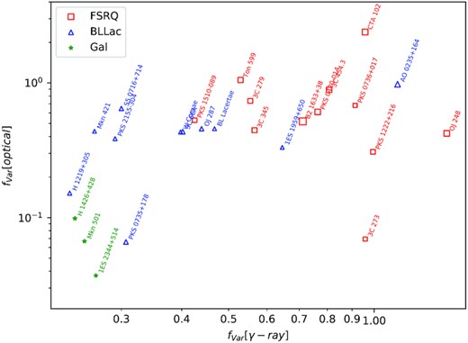
Optical fractional variability versus HE γ-ray fractional variability of the blazar sample. Green stars represent those blazars dominated by the stellar emission of the host galaxy, blue triangles correspond to BL Lac objects, and red squares to FSRQs. The size of the symbols is proportional to the redshift of the object.
Sample of blazars from the Steward Observatory monitoring program included in the NMF analysis.
| (1) | (2) | (3) | (4) | (5) | (6) | (7) | (8) | (9) | (10) | (11) | (12) | (13) | (14) | (15) |
|---|---|---|---|---|---|---|---|---|---|---|---|---|---|---|
| Source | Type | No. of | No. of | Fvar | |$\sigma ^{2}_{\text{exp}}$| | |$\sigma ^{2}_{1}$| | |$\sigma ^{2}_{2}$| | |$\sigma ^{2}_{3}$| | |$\sigma ^{2}_{4}$| | α1 | α2 | α3 | α4 | Colour |
| spectra | components | (per cent) | (per cent) | (per cent) | (per cent) | (per cent) | ||||||||
| Mkn 501 | Galaxy dominated | 476 | 2 | 0.067 ± 0.001 | 95.87 | 25.36 | 70.51 | – | – | – | 1.40 | – | – | BWB |
| H 1426+428 | Galaxy dominated | 36 | 2 | 0.099 ± 0.006 | 96.46 | 25.86 | 70.60 | – | – | – | 1.33 | – | – | Achromatic |
| 1ES 2344+514 | Galaxy dominated | 81 | 2 | 0.038 ± 0.007 | 88.60 | 30.13 | 58.49 | – | – | – | 0.99 | – | – | BWB |
| 3C 66A | BL Lac | 353 | 3 | 0.434 ± 0.002 | 99.91 | 27.93 | 34.43 | 37.55 | – | 0.84 | 1.15 | 1.48 | – | BWB |
| AO 0235+164 | BL Lac | 207 | 2 | 0.978 ± 0.008 | 98.00 | 15.82 | 82.18 | – | – | −0.14 | −0.57 | – | – | RWB, FWB |
| S5 0716+714 | BL Lac | 226 | 3 | 0.646 ± 0.002 | 99.98 | 30.70 | 63.05 | 6.23 | – | 0.87 | 1.17 | 0.04 | – | BWB |
| PKS 0735+178 | BL Lac | 34 | 2 | 0.066 ± 0.004 | 96.74 | 37.62 | 59.12 | – | – | 0.65 | 1.36 | – | – | BWB |
| OJ 287 | BL Lac | 516 | 4 | 0.457 ± 0.001 | 99.88 | 28.57 | 17.68 | 36.86 | 16.78 | 0.81 | 0.99 | 1.19 | 0.46 | FWB |
| Mkn 421 | BL Lac | 594 | 2 | 0.438 ± 0.002 | 99.95 | 14.48 | 85.47 | – | – | 0.96 | 2.15 | – | – | BWB |
| W Comae | BL Lac | 345 | 3 | 0.432 ± 0.002 | 99.86 | 17.01 | 74.20 | 8.65 | – | 0.43 | 1.13 | 0.18 | – | BWB |
| H 1219+305 | BL Lac | 34 | 3 | 0.152 ± 0.007 | 98.23 | 19.82 | 29.53 | 48.88 | – | 0.91 | 1.26 | 0.72 | – | No trend |
| 1ES 1959+650 | BL Lac | 147 | 2 | 0.332 ± 0.003 | 99.80 | 16.73 | 83.07 | – | – | 0.55 | 1.48 | – | – | BWB |
| PKS 2155−304 | BL Lac | 299 | 4 | 0.386 ± 0.003 | 99.85 | 19.28 | 43.64 | 14.89 | 22.05 | 1.32 | 1.63 | 1.85 | 1.20 | BWB |
| BL Lacertae | BL Lac | 699 | 4 | 0.457 ± 0.001 | 99.71 | 16.08 | 40.39 | 9.07 | 34.17 | 0.25 | 0.69 | 0.05 | 0.72 | BWB |
| PKS 0420−014 | FSRQ | 53 | 3 | 0.610 ± 0.006 | 99.83 | 0.72 | 83.69 | 15.41 | – | – | 0.89 | 0.32 | – | RWB, BWB |
| PKS 0736+017 | FSRQ | 126 | 4 | 0.682 ± 0.006 | 99.72 | 2.68 | 61.06 | 33.98 | 2.01 | – | 0.92 | 0.50 | 3.49 | No trend, FWB |
| OJ 248 | FSRQ | 224 | 3 | 0.422 ± 0.005 | 99.48 | 1.20 | 59.23 | 39.06 | – | – | 1.33 | 1.06 | – | No trend, FWB |
| Ton 599 | FSRQ | 190 | 4 | 1.052 ± 0.004 | 99.96 | 0.05 | 72.55 | 14.38 | 12.98 | – | 1.37 | 1.74 | 0.94 | RWB, FWB |
| PKS 1222+216 | FSRQ | 427 | 4 | 0.308 ± 0.006 | 99.75 | 11.72 | 71.03 | 4.34 | 12.65 | – | 1.70 | 3.65 | 0.52 | RWB, FWB |
| 3C 273 | FSRQ | 298 | 3 | 0.069 ± 0.008 | 97.01 | 0.75 | 45.03 | 51.23 | – | – | 4.18 | 4.41 | – | BWB |
| 3C 279 | FSRQ | 499 | 4 | 0.736 ± 0.002 | 99.90 | 0.01 | 32.85 | 19.22 | 47.74 | – | 1.20 | 1.59 | 1.05 | No clear trend |
| PKS 1510−089 | FSRQ | 371 | 3 | 0.529 ± 0.003 | 99.43 | 4.77 | 89.27 | 5.38 | – | – | 1.24 | 2.52 | – | RWB |
| B2 1633+38 | FSRQ | 362 | 3 | 0.519 ± 0.005 | 99.51 | 3.11 | 91.21 | 5.19 | – | – | 1.23 | 2.34 | – | RWB |
| 3C 345 | FSRQ | 42 | 3 | 0.446 ± 0.021 | 98.96 | 11.93 | 63.06 | 23.98 | – | – | 1.39 | 1.25 | – | RWB |
| CTA 102 | FSRQ | 287 | 4 | 2.392 ± 0.005 | 99.98 | 0.25 | 98.93 | 0.25 | 0.56 | – | 1.23 | 0.94 | 0.57 | RWB, FWB, BWB |
| 3C 454.3 | FSRQ | 549 | 3 | 0.89 ± 0.002 | 99.90 | 4.25 | 78.48 | 17.17 | – | – | 0.86 | 0.54 | – | RWB, BWB |
Columns. (1) Target name; (2) source type; (3) number of spectra available; (4) number of reconstructed components; (5) fractional variability and its uncertainty; (6) percentage of explained variance; (7–10) percentage of variance explained by each component; (11–14) spectral index of the n component; (15) long-term colour trends. When more than one trend is reported, it goes from lower to higher flux states.
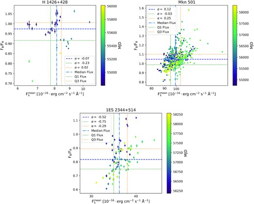
Colour–flux diagrams for galaxy-dominated blazars. The colour is estimated as the ratio between the blue and red parts of the spectra. Thus, higher colour values represent bluer spectra. The vertical dash–dotted line corresponds to the median flux. Vertical dotted lines represent the first and third quartiles for the flux values. The horizontal dashed line denotes the median colour value, and its corresponding spectral index is noted in the legend. Horizontal dotted lines represent the first and third quartiles of the colour and their corresponding spectral index are noted in the legend.


Colour–flux diagrams for BL Lac objects. The colour is estimated as the ratio between the blue and red parts of the spectra. Thus, higher colour values represent bluer spectra. The vertical dash–dotted line corresponds to the median flux. Vertical dotted lines represent the first and third quartiles for the flux values. The horizontal dashed line denotes the median colour value, and its corresponding spectral index is noted in the legend. Horizontal dotted lines represent the first and third quartiles of the colour and their corresponding spectral index are noted in the legend.


Colour–flux diagrams for FSRQs. The colour is estimated as the ratio between the blue and red parts of the spectra. Thus, higher colour values represent bluer spectra. The vertical dash–dotted line corresponds to the median flux. Vertical dotted lines represent the first and third quartiles for the flux values. The horizontal dashed line denotes the median colour value, and its corresponding spectral index is noted in the legend. Horizontal dotted lines represent the first and third quartiles of the colour and their corresponding spectral index are noted in the legend.
Figs 2 and 3 reveal that almost all the BL Lac objects of this sample agree with the historical BWB trends observed in this blazar type, as well as the three galaxy-dominated blazars studied here. However, some atypical cases are found in these objects: AO 0235+164 shows different trends, more similar to those found in FSRQs; OJ 287 shows no clear behaviour in the colour except for an achromatic brightening; and 3C 66A displays a subset of spectra deviating from the general BWB trend of the rest of the data sample. These behaviours will be discussed in more detail in Section 5.
FSRQs show the RWB trend mentioned before (see Fig. 4). However, more complicated colour behaviours can be seen in this blazar type, with colour flattening and even BWB trends during the highest emission states for some sources. In almost all the FSRQs, we observe this RWB trend, followed by a flatter-when-brighter (FWB) behaviour during bright outbursts, once the flux rises over a certain saturation value. The RWB trends in these objects show a large colour change with small flux changes. This is associated with flux changes during low states of these sources, which also imply large changes in their spectral slopes (Dai et al. 2009). Moreover, only three sources of the data set (3C 454.3, CTA 102, and PKS 0420−014) display a clear BWB evolution during a high flux state. This behaviour will be discussed in Sections 5 and 6 in the framework of their more complicated morphology, the different acceleration/cooling processes taking place in the jet, and the relative contributions of the different components.
4 METHODOLOGY
4.1 Non-negative matrix factorization
The main advantage of the NMF with respect to other dimensionality reduction algorithms such as the PCA is that the data, weights and components must be non-negative (Blanton & Roweis 2007). While PCA components must be orthogonal and thus, some of them may have negative values, making a physical interpretation more difficult, the NMF leads to an easier physical association due to the non-negative restriction. However, this non-orthogonality condition has also the caveat of resulting in degeneracy of the components. In this work, we make use of the NMF algorithm implemented in the python package scikit.4
4.2 Reconstruction of the data sample
Previous works using the NMF are based on a reconstruction with a number of components estimated from the residual sum of squares (RSS) diagram (see e.g. Hutchins et al. 2008). The RSS is a measurement of the discrepancy between the data and the model (see Fig. 5). The RSS of pure random noise follows a decreasing linear trend as the number of components increases. Those points deviating more than 5σ from this linear trend correspond to the components that represent real variability and consequently, the minimum number of components needed for the reconstruction of the data. No a priori information is given to the algorithm. This approach results in a total number of two components needed for most of the BL Lac and galaxy-dominated objects, and three components for almost all of the FSRQs of the sample.
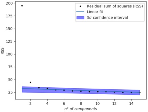
RSS versus number of components for the BL Lac object PKS 2155−304. The number of components needed for the reconstruction is estimated by a linear fit of the RSS. The amount of components needed is equivalent to the number of points that deviate from the 5σ confidence interval of the fit.
While this procedure maximizes the variance explained by the reconstruction, the components contain mixed contributions and the physical interpretation of the components is not straightforward. This methodology leads to resulting components in which the emission of different regions of the AGN are mixed into an individual component (e.g. PL-type component with characteristic BLR emission lines; see Fig. 6). This effect makes hard to obtain a physical interpretation of the reconstruction and to quantify the amount of variability that is caused by each constituent of the AGN.
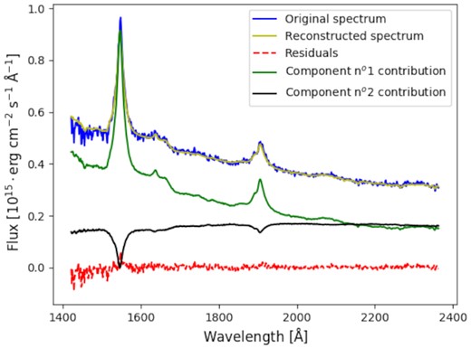
Reconstructed spectrum of the FSRQ B2 1633+38. Two components are used for the reconstruction, without any a priori assumption. The first component represents the emission coming from the BLR. The second component shows artificial absorption lines non-existent in the total spectrum, introduced by the NMF to minimize the residual.
In this paper, we propose a complementary methodology for the reconstruction of the spectra of the sources. This approach is based on the a priori knowledge of the possible components we can expect from the different types of blazars:
BL Lacs: The absence or minor presence of signatures of an accretion disc, dusty torus, or a BLR in BL Lac objects makes the relativistic jet the main contribution (e.g. Plotkin et al. 2012). The synchrotron emission coming from the jet can be described as a PL function in a narrow spectral range. For larger spectral ranges, other models (e.g. log-parabola) may be more adequate.
FSRQs: Apart from the dominant non-thermal emission from the jet, these sources exhibit broad optical emission lines coming from the BLR (see e.g. Ghisellini & Tavecchio 2008) and likely thermal emission from the accretion disc (e.g. Shang et al. 2005; Calderone et al. 2013). In this case, we use a quasi-stellar object (QSO) emission to account for the BLR and a set of PLs to describe the main contribution of the jet, and the accretion disc.
Galaxy-dominated sources: In some cases, the jet of BL Lacs is not bright enough to outshine the host galaxy. In such objects, the emission of the stellar population can be the principal contribution to the optical emission (see e.g. Massaro et al. 2015). For these sources, the stellar population and the jet contributions are expected.
Under these considerations, we propose an approach that consists in using these a priori expected components to reconstruct the spectra data set of each target. These components are fixed and used as input for the reconstruction, and the NMF algorithm estimates the overall contribution of each one for all the spectra. This method also solves the degeneracy caveat that can be introduced by the non-orthogonality condition of the NMF. The initial number of components is estimated with the RSS diagram. After a first reconstruction, a residual map is inspected to account for the success of the global reconstruction (see e.g. Fig. 7). In case an extra component is needed to explain the variability of a certain source, it can be easily identified in the residual map and added to the reconstruction. Colour/spectral index changes in the data set can be identified as a region of the residual map with a positive (negative) residual in the blue part of the spectrum, and negative (positive) residual in the red part. To quantify if a reconstruction is accurate enough or if an additional component is needed, we estimate the squared errors of each reconstructed spectrum. If more than 5 per cent of the whole set of spectra is above a 5σ threshold with respect to the noise of each spectrum in the data set, another component is added to the reconstruction. On the other hand, if more than 95 per cent the data set is below this limit value, the reconstruction is considered to be satisfactory. It is important to note that, for those sources with a reduced amount of spectra, a visual inspection of the residual map is specially important to evaluate if another component is needed. In those cases, we check if the spectra showing high residuals are clustered within a time period, indicating a true deviation, while isolated cases are less significant.
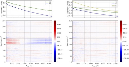
Residual map for the reconstruction of 3C 66A. Left-hand panels: reconstruction with two components. Right-hand panels: reconstruction with three components. Red and blue colours indicate the spectra for which the reconstruction is not accurate and where an extra component is needed to reproduce the data set. The top panels show the components used for the reconstruction in each case.
4.2.1 Reconstruction of Galaxy-dominated blazars
The reconstruction of spectra dominated by the host galaxy emission can be used as a test of our methodology, since the derived contribution of the stellar population should remain fairly constant. As established above, in the case of galaxy-dominated sources the optical spectrum is mostly contributed by the host galaxy emission plus a variable part from the jet. The RSS diagram suggests a reconstruction based in two components to reproduce the variability of these objects. The stellar emission is derived using the penalized pixel fitting (pPXF) method (Cappellari & Emsellem 2004; Cappellari 2017). In order to derive the best stellar population template, we use the mean spectrum derived for each of the three objects. To better adjust the continuum shape of the spectrum and account for the featureless synchrotron contribution, we include an additive polynomial during the fit. The best-fitting stellar population templates correspond in all cases to an old stellar population (|$\gtrsim 11\, \mathrm{Gyr}$|) and metallicity slightly higher than the solar value. Similar results are found when using spectra representing the low state of each object. To model the contribution of the jet we use the polynomial function result of the pPXF to describe this continuum component.
4.2.2 Reconstruction of BL Lac objects
BL Lac objects are characterized by the dominance of the jet over any other component, and by an (almost) featureless spectrum. Thus, we use a reconstruction based on different PLs (Fλ ∝ λ−α) to account for the change of slope of the spectra. These PL functions have a fixed spectral index, but can vary in flux. Thus, combinations of the different PL functions account for the spectral changes, while their flux scales are related to their relative contribution to the emission. We find that, for most of the BL Lac objects, an initial number of two components is needed for the reconstruction. Then if needed, we add more PL components, to explain periods of residual excess due to strong spectral changes.
The initial PL type components are estimated from the maximum and minimum spectra (computed as the mean of the percentile 90 and percentile 10 spectra, respectively). The minimum spectrum is taken as the first component, while the difference between the maximum and the minimum spectra is used as the second one. Thus, if a BL Lac shows any emission/absorption lines in its spectrum, it will appear associated with the first component. This is due to the fact that these lines will be more visible during low states. If an extra component is required when an excess appears in the residual map of a subset of spectra (usually coincident with colour/spectral index changes as shown in Fig. 7), it is added as the median of this subset.
4.2.3 Reconstruction of FSRQs
FSRQs show broad emission lines in their optical spectra due to the presence of the BLR in the surroundings of the black hole. Therefore, we need to add a component that accounts for the presence of these lines in the spectra. Moreover, FSRQs often show an excess in the optical/ultraviolet (UV) part of their spectrum known as the blue bump, introduced by the accretion disc. The presence of the BLR and accretion disc makes the number of components derived from the RSS representation higher than in the BL Lacs case. The methodology applied in this work leads to a reconstruction that needs three or more components to model and reproduce the variability observed in FSRQs.
In order to define the a priori components for the FSRQs, we make use of the QSO template from Vanden Berk et al. (2001) to account for the emission lines in the spectra. The mean spectrum is fitted to a sum of a PL component that describes the emission of the jet, and the QSO template. Then, the final template, used as input to the NMF, is derived as the difference between the mean spectrum and the fitted PL. In this way, the template derived for each source matches better the intensity/profile of the emission lines of each FSRQ. The derived contribution of this component is expected to remain mostly constant. However, if long-term variations are observed, it may indicate intrinsic variation of the BLR + accretion disc emission. The fitted PL is used as the second component. Finally, an additional PL is added to model changes of the spectral index. This third component is estimated from the subset of spectra with significant spectral change as for BL Lac objects, after subtracting the estimated QSO template contribution.
5 RESULTS
In this section and Section 6, we report the general results and the interpretation for all the sources of each type included in the analysis. A detailed discussion on some individual sources of special interest can be found during the following subsections and some notes on the rest of the sample are found in Appendix A. The results of the reconstructions are summarized in Table 2.
5.1 Galaxy-dominated sources
Galaxy-dominated blazars are characterized by a much smaller variability with respect to BL Lac objects and FSRQs. Their fractional variability in the optical band is significantly smaller compared to the latter blazar types (see Fig. 1). This fact, along with the dominance of the host galaxy over the other parts of the AGN, makes them appropriate targets to test the reliability of the adopted methodology, since the expected stellar contribution should remain constant. The three blazars dominated by the stellar emission of the host galaxy were reconstructed with two components: the stellar emission template to account for the bright host galaxy, and the PL component responsible for the synchrotron emission of the jet. We find that we are able to reconstruct accurately the emission and variability of these blazars using these two simple components. These objects show a mild BWB behaviour in their colour evolution with the flux (see Fig. 2). This trend comes from the second component of the reconstruction, associated with the non-thermal synchrotron emission of the jet. In the following subsection, we discuss the results of Mkn 501 as an example of this blazar type. The discussion about H 1426+428 and 1ES 2344+514 can be found in Appendix A1.
5.1.1 Mkn 501
The results of the NMF reconstruction of Mkn 501 can be seen in Fig. 8. This blazar displays a very low variability in optical frequencies (|$F_{\rm var}=10{{\ \rm per\ cent}}$|) that is also consistent with the low variability reported in the 4LAC-DR2 Fermi-LAT catalogue. This is a consequence of Mkn 501 being a high-synchrotron peaked (HSP) blazar, so the variability is stronger after the SED bumps (X-rays and VHE γ-rays). The host galaxy of Mkn 501 contributes with 40 per cent of the overall optical flux (see Fig. 8). The component C1 corresponds to a galaxy with an old stellar population and its derived mean flux contribution does not show significant variation. C2 is a PL with a moderate slope and it is responsible for the observed spectral variability. It also accounts for the observed colour variations, in all cases BWB. The colour of this blazar shows two long-term BWB trends due to the same behaviour observed in the second component of the reconstruction, associated with the jet. The presence of different BWB trends due to different states of this sources was also found by other studies (e.g. Xiong et al. 2016). We also note by looking at Fig. 8 that in the period between MJD 56400 and MJD 56800, there is a small residual excess. This period is coincident with a rapid bluer trend, not accompanied however by a flux increase. This may indicate that a third component may be needed to reconstruct this small subset.
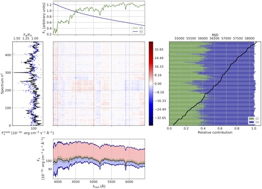
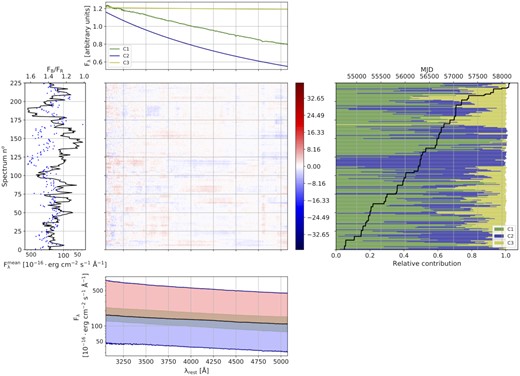
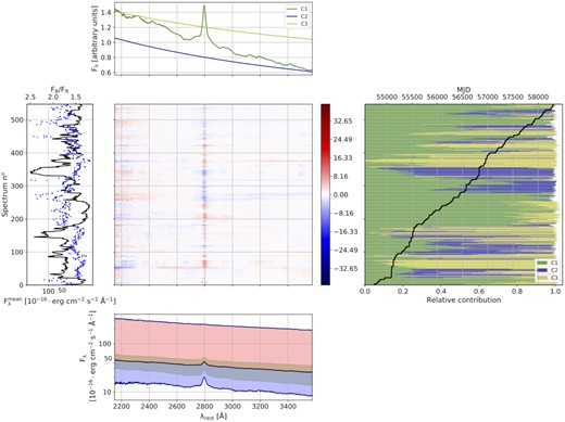
Results of Mkn 501. Top panel: normalized components. Middle panels: residual map. The colour scale is estimated in terms of the noise of each spectrum. Bottom panel: median (black), minimum, and maximum (dark blue) spectra. The variability range between the maximum (minimum) and the median spectra is represented by the red (light blue) contour, and the variability range between the percentiles 25 and 75 with the green contour. Right-hand panel: relative contribution of each component. The black line represents the MJD of each spectrum. Left-hand panel: mean flux and colour of each spectra. Blue dots correspond to the colour of each spectrum.
5.2 BL Lac objects
BL Lac objects are reconstructed using two to four components depending on the amount of spectral variability of the source. These components are able to explain more that 99 per cent of the variance of the original data set and thus, to model accurately the variability observed in these blazars. Typically the different components obtained from the analysis dominate the emission as the colour changes, reproducing also the spectral evolution of the source. The BL Lac objects used in this analysis are also characterized by a BWB behaviour (as shown in Fig. 3), followed by almost all the targets of this type (see Fig. 3).
Specially remarkable are the cases of the BL Lac objects AO 0235+164, OJ 287, and S5 0716+714. These objects have shown colour behaviours different to the general BWB trend associated with BL Lacs. In addition, OJ 287 is an interesting blazar since it is thought to host a binary system of two supermassive black holes. Furthermore, the appearance of transient components propagating along the jet can be identified in sources such as 3C 66A. A detailed discussion on the results of these sources is included in the following subsections. Mkn 421 is also reported in this section as a prototype of the BL Lac blazar type. An overview of the rest of the BL Lac objects can be found in Appendix A2.
5.2.1 3C 66A
The reconstruction of the available spectra is done using three PL components (see Fig. 9). The fraction of explained variance attributed to each component is nearly equal, corresponding to about 33 per cent. The first component is the flattest one and its contribution to the total flux is above one-third for about 80 per cent of the time, contributing even more when the source is at its low state. The second component has an intermediate slope and appears dominant when the source is at relatively high state, although its contribution is not exceeding 60 per cent. The third component shows the steepest slope and dominates the spectra (|$\sim 90{{\ \rm per\ cent}}$|) for the period between MJD 56250–56700 and also shortly in the period MJD 57700–57750. The results of the reconstruction are presented in Fig. 9.
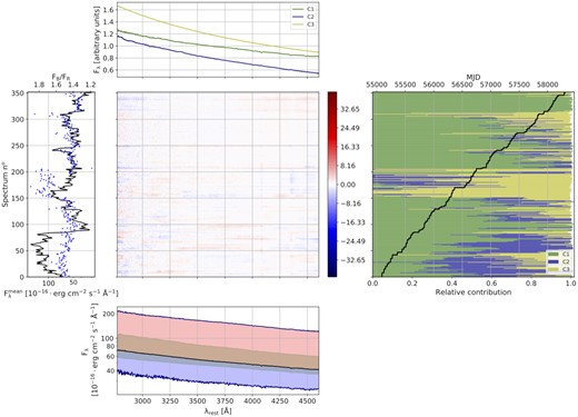
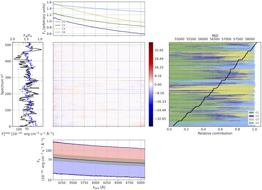
Results of 3C 66A (same description as Fig. 8).
This source presents an overall BWB behaviour, which has been also reported in previous studies (e.g. Meng et al. 2018). This trend can be related mostly to the second component. This component clearly modulates the BWB behaviour, as it increases more during the bluest spectra, and fades by one order of magnitude when the spectra become redder. On the other hand, the first component was found to be roughly constant and achromatic. Moreover, the third component also shows this BWB trend. However, it is representative only for a reduced amount of spectra. This reduced subset is also characterized by a significant change of the spectral index and colour, disconnected from the overall behaviour of the rest of the data set. This can be interpreted as a transient component propagating along the jet that dominates the emission during a short period of time compared to the time span covered by the full data set (Wang et al. 2022).
5.2.2 AO 0235+164
The results of the NMF analysis of AO 0235+164 are shown in Fig. 10. The RSS diagram indicates that two components are enough to explain most of the observed variance. An inspection of the residuals also reveals that two components are sufficient to have a good reconstruction of the spectra with the adopted methodology. The flux of this source is nearly constant during its low state, increasing significantly during two outburst events in which the second component becomes the brightest. The first component is nearly flat and it is dominant when the source is at low state (35 per cent of the spectra) and accounts for only 15 per cent of the variance. It also shows the broad Mg ii λ2800 line, that becomes clearly visible during low-activity states. The second component is very similar to a red PL, being dominant for about 65 per cent of the spectra and it accounts for 80 per cent of the variance. The combination of these two components accounts for the double-trend colour variation with flux (see Fig. 3), more similar to that observed in FSRQs. The brightest spectra show a very mild BWB trend, almost flat, while the low state of the source displays an RWB trend. We note that the PL indices of these components show a negative value, being the only ones in our sample (see Table 2). This is likely due to the extinction produced by the intervening absorber at z = 0.524 (AV = 0.99 derived by Junkkarinen et al. 2004; Raiteri et al. 2005), which has not been corrected for here.
Results of AO 0235+164 (same description as Fig. 8).
Previous studies have reported for this source an FSRQ-like behaviour, with RWB trends in the colour, contrary to the typical BWB relation observed in BL Lacs (Raiteri et al. 2014). Bonning et al. (2012) detected a more complicated colour evolution, with two different states depending on the observed γ-ray intensity. In addition, the optical spectra of AO 0235+164 taken during the low states displayed by this object reveal a prominent and broad emission line, that disappears during the flaring states. These features, more common in FSRQs, may indicate that AO 0235+164 could be a transitional blazar. In this framework, the two components obtained by the NMF reconstruction can be interpreted as a first component with the contribution of a weak BLR, responsible for the FSRQ-like behaviour, and a second component that explains the emission from the jet and it is responsible of the BL Lac-type FWB behaviour and the flaring states of this object (Raiteri et al. 2006). Other authors have also proposed the existence of two components to reproduce the variability of this blazar, as well its colour behaviour (see e.g. Raiteri et al. 2006; Cellone et al. 2007). Bonning et al. (2012) also consider the possibility of the presence of an accretion disc contributing to the optical-IR emission in this source.
5.2.3 S5 0716+714
The spectral variability of this blazar is reconstructed with three components that reproduce 99.98 per cent of its variability. The results of this reconstruction can be seen in Fig. 11. C1 contributes with more than one-third of the emission in about 2/3 of the spectra. Its contribution to the |$\sigma ^2_{\rm exp}$| is around 30 per cent. C2 is the bluest component and it is responsible for about 65 per cent of the |$\sigma ^2_{\rm exp}$|. It shows the larger contribution to the mean flux during the decline of bright flares. C3 is an almost flat PL and it is responsible for about 6 per cent of the |$\sigma ^2_{\rm exp}$|, indicating that it remains basically constant. Its contribution to the mean flux is large (up to 50 per cent) when the C2 contribution vanishes, otherwise its contribution stays around 20 per cent.
Results of S5 0716+714 (same description as Fig. 8).
S5 0716+714 does not show overall any clear colour trend (see Fig. 3). However, at shorter time-scales it shows the typical BWB trend of BL Lacs, associated with the bright flares observed in the left-hand panel of Fig. 11. The peculiarity about its colour evolution is that this BWB displays three different trends with three slopes, associated with three different brightening periods: a very steep BWB behaviour for the faintest spectra; a second trend with higher flux variations and lower colour change; and a third trend with lower colour variability that corresponds to the highest flare observed in this blazar during the 10-yr monitoring (MJD 57046). The existence of multiple trends in the colour evolution can be an indicative of different electron populations responsible for the synchrotron emission, or can be associated with different activity levels of the source (Xiong et al. 2016). In terms of the individual components, these trends are related to the second component, which is the bluest and showing the different trends identified in the overall behaviour. On the other hand, the first and third component vary uncorrelated with the colour of the spectra.
5.2.4 OJ 287
The RSS indicates a total of two components. However an inspection of the residual map reveals additional components. The best reconstruction with our approach is obtained using four components, which are PLs of spectral indices ranging from 0.5 to 1.2. The results of this reconstruction are shown in Fig. 12. All components contribute significantly to the |$\sigma ^2_{\rm exp}$|: C1 and C3 have a higher contribution, reaching about 28 and 35 per cent of the |$\sigma ^2_{\rm exp}$|, respectively, whereas C2 and C4 contribute the least, around 15 per cent of the variance. C1 contributes more than 30 per cent to the total flux for about one-third of the spectrum set and it dominates basically when the source is at lower states. C3 shows the steepest slope and it is dominant within the periods MJD 56400–56650 and 57650–57900. C4 has the shallowest slope, i.e. the reddest colour, and it contributes mostly during the periods MJD 54750–55000 and 57250–57400. C2 has a relative contribution of 30 per cent of the flux associated with the higher states of the source, and coincident when C4 is not contributing significantly. OJ 287 exhibits large colour variability during the monitoring period. However, contrary to the common behaviour observed in BL Lac-type blazars, this variability appears uncorrelated with flux changes. This can be understood in terms of the component slopes, which are very similar for C1, C2, and C3, which have the highest contributions. The exception to this behaviour happened during the bright flare occurring between MJD 57650 and MJD 57900, showing a very interesting behaviour in the optical regime. This episode exhibits an FWB colour trend. The activity appears to start around MJD 57250, when the spectrum becomes bluer. During this episode the component C3 contributes almost 100 per cent and the flux increases roughly achromatically. During this period the spectra can be reconstructed by a combination of C1 and C4. At MJD 57700, the decrease of flux starts and the spectrum is formed by C2 and C3 as basic contributors. After MJD 58000 the flux returns to a low state and the spectra are reconstructed by a large contribution of C1, plus C2 and C4 with lower contributions. The fact that these three components have similar indices and relative contributions may also indicate that they represent the component of the jet, but varying the energy of the electrons responsible for the emission.
Results of OJ 287 (same description as Fig. 8).
OJ 287 is a well-known BL Lac object, thought to host a binary supermassive black hole system, showing major outbursts approximately every 12 yr (Sillanpaa et al. 1988), with a structure of two peaks separated by ∼1–2 yr. Several models have been proposed to explain the behaviour observed in this object. The flare observed in our data is predicted by the binary model (Valtonen et al. 2016; Kapanadze et al. 2018). A detailed discussion of the different binary black hole models and their limitations can be found in (Sillanpaa et al. 1996). Sillanpaa et al. (1988) suggested a model where the flares are produced by the secondary black hole crossing the accretion disc of the primary, inducing tidal perturbations in the disc. This variant is able to predict the flares and reproduce their colour stability, as the energy production mechanism is expected to remain unchanged. However this binary BH model is not able to explain the appearance of a double peak during the flares. On the other hand, the variant proposed by Lehto & Valtonen (1996) is able to accurately predict the consecutive outbursts every 12 yr and reproduce the double-peak structure. However, they fail when explaining the achromatic development of the flares, since, in this model, the energy production mechanism is expected to change during these events, as the flares in this model are produced by thermal outburst in the disc. Another plausible variant, suggested by Villata et al. (1998), is based on strongly bent jets emerging from both BHs, in which the periodicity is caused by the beaming effects. This model is able to explain both the double peak structure of the flares and the achromatic brightening, as long as the energy production is the same in both jets. Alternatively, Bonning et al. (2012) interpret the achromatic brightenings in blazars as pure geometrical effects, which could explain the behaviour observed in this object. The components found in our NMF decomposition do not indicate the presence of a thermal component, favouring those models in which the emission is coming from the relativistic jet.
5.2.5 Mkn 421
Mkn 421 is reconstructed by two PL-like components to account for the emission of the powerful jet, as shown in Fig. 13. The colour-flux diagram shows a clear BWB trend, and during the brightest state shows a large blue colour increases, without almost no flux change, as shown in Fig. 3. The first component, C1, contributes above 50 per cent to the mean flux most of the time, except for the period MJD 56250–56750, when the component C2 becomes fully dominant. This corresponds to the bluest spectra shown by Mkn 421, which are consistent with the BWB behaviour, already reported by Carnerero et al. (2017). The first component does not vary dramatically, it accounts for |$\sim 15{{\ \rm per\ cent}}\, \sigma ^2_{\rm exp}$| and its contribution remains constant even when colour changes. C2 accounts for most of the variability of this source (|$\sim 85{{\ \rm per\ cent}}\, \sigma ^2_{\rm exp}$|). This component is also responsible for the BWB behaviour of this blazar (see Fig. 3). The two-component decomposition of the data set is supported by a two-zone scenario used in several studies for this blazar in the past (see e.g. Aleksić et al. 2015).

Results of Mkn 421 (same description as Fig. 8).
5.3 FSRQs
The NMF reconstruction of FSRQs requires at least three components to explain more than 99 per cent of the observed variability. This difference with the BL Lac objects is due to the presence of a bright BLR in FSRQs. We observe an RWB trend in most of the FSRQs, historically associated with this blazar type (see Fig. 4). We also identify an FWB behaviour during bright outburst events, when the source overcomes a certain flux. For three of the FSRQs, we also detect a BWB following the colour flattening: PKS 0420−014, 3C 454.3, and CTA 102. Furthermore, among the FSRQs studied here there are two objects with a peculiar colour variability: 3C 273 and 3C 279. The former shows a long-term BWB evolution in its colour variations, with different trends at shorter time-scales. Such behaviour was already reported in the past for 3C 273 by Dai et al. (2009) in both intraday and long-term time-scales. The latter on the other hand, shows a much more complex behaviour. Furthermore, some of the FSRQs studied here (e.g. PKS 1222+216) show rather steep and less variable components with no correlation with the overall flux that can be associated with a bright accretion disc. The results of 3C 273, 3C 279, 3C 454.3, CTA 102, and PKS 1222+216 are discussed within the following subsections. The rest of the FSRQs of the sample are included in Appendix A3.
5.3.1 PKS 1222+216
The reconstruction of the FSRQ PKS 1222+216 is based on a total of four components. The results obtained for this blazar are shown in Fig. 14. The first one, associated with the BLR, represents the higher contribution (|$\gtrsim 80{{\ \rm per\ cent}}$|) to the optical emission of this blazar, except for the period between MJD 56250 and 57250. The component C1 shows some of the HI Balmer lines and at the blue end, the red wing of the Mg ii 2800. C2 contributes about 50–60 per cent for the period MJD 56600–56750, coincident with a large flare. It is the most variable component, accounting for 70 per cent of |$\sigma ^2_{\rm exp}$|. It also has a relatively steep slope (α = 1.70). On the contrary, C4 shows an almost flat slope (α = 0.52). This component becomes important during the decline of the big flare, starting around MJD 56760 until MJD 57400. The component C3, much steeper than C2 and C4 (α = 3.65), shows the largest contribution in the period MJD 56250–56400. It remains relatively constant during this period (4 per cent |$\sigma ^2_{\rm exp}$|). This fact and its very steep slope may be indicative of emission coming from the accretion disc in the form of the Big Blue Bump, similarly to the case of 3C 273 (see Section 5.3.2).

Results of PKS 1222+216 (same description as Fig. 8).
The overall colour behaviour of PKS 1222+216 reveals an RWB trend, followed by a hint of the colour saturation observed in other FSRQs. This RWB evolution is caused by the combination of C2 and C4, also showing this same trend. These components become dominant when the source enters a high state. At low states, C3 dominates over C2 and C4, remaining mostly constant. This is compatible with its association with the bright accretion disc, suggested above. When the synchrotron emission, explained through C2 and C4, equates the blue bump of the accretion disc (C3), a flattening of the RWB trend and posterior colour saturation is observed, as the jet contribution overcomes the accretion disc one.
5.3.2 3C 273
The optical spectra of this source do not show much variability (|$F_{\rm var} \sim 10{{\ \rm per\ cent}}$|). Our NMF decomposition consists of three components accounting for about |$97{{\ \rm per\ cent}}$| of |$\sigma ^2_{\rm obs}$|. The NMF reconstruction of this source is shown in Fig. 15. The first component, C1, is associated with the BLR and varies very little (|$\lesssim 1{{\ \rm per\ cent}}\sigma ^2_{\rm exp}$|), although its contribution to the optical flux is around 40–50 per cent over the whole period. The other two components, C2 and C3, contribute almost equally to the |$\sigma ^2_{\rm exp}$| and are approximated by very steep blue PLs. C2 contributes among 50–60 per cent to the total flux for about 75 per cent of the spectrum set. C3 appears only for certain periods, e.g. MJD 56250–56750. During these periods, C3 becomes important when C2 becomes negligible. Raiteri et al. (2014) modelled the SED in the optical near-IR range by adding an extra blackbody component attributed to a bright accretion disc, apart from the QSO template. Our components C2 and C3 may correspond to this blackbody emission coming from the accretion disc. These two components may be associated with two different states of the disc, corresponding to variations in the accretion rate (Li et al. 2020).

Results of 3C 273 (same description as Fig. 8).
Contrary to the general behaviour of the FSRQs studied here, this blazar displays a clear BWB long-term evolution. This makes 3C 273 the only blazar of the sample with such behaviour. Dai et al. (2009) have also observed this trend in the past, in both intraday and long-term time-scales. While we do not have the temporal coverage to evaluate the intraday colour variability, we do see different BWB slopes on time-scales shorter than a year.
5.3.3 3C 279
The reconstruction of 3C 279 requests four components that are able to model 99.91 per cent of its variability during this 10-year period. The results of the analysis of 3C 279 can be seen in Fig. 16. The NMF analysis on this source reveals a very faint BLR component (C1), which does not contribute more than 5-10 per cent to the mean flux. Weak emission lines (Mg ii 2800, [O ii]3727, and [Ne iii]3869) become evident during the low state of the source. Its contribution to the |$\sigma ^2_{\rm exp}$| is very low (∼0.01), indicating that it remains constant in the whole spectrum set. When 3C 279 displays an enhanced state, this component remains almost invisible due to the high dominance of the jet. The component C2 is responsible for about 33 per cent of the |$\sigma ^2_{\rm exp}$|. It is a PL showing an intermediate slope compared to C3 (steepest) and C4 (flattest). Its relative contribution to the mean flux of the spectra ranges from 50 to 90 per cent, excluding the period from MJD 55200 to 55900, when C4 contributed most (∼90–100 per cent). The component C4 becomes dominant over shorter periods when C2 diminishes. C4 is the most variable, accounting for about 48 per cent of the |$\sigma ^2_{\rm exp}$| and shows a slope flatter than C2. The component C3 is the PL showing the steepest slope and accounts for about 20 per cent of |$\sigma ^2_{\rm exp}$|. It is responsible of the bluest spectra, occurring in the period of MJD 56250–56750. We note that despite the goodness of the reconstruction, for the minimum spectra there is still some residual that is not being reconstructed. This may be caused by the higher noise and fluctuations of this subset of spectra.
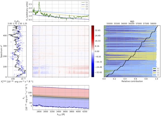
Results of 3C 279 (same description as Fig. 8).
Contrary to the bulk of the FSRQ population, 3C 279 does not show any clear long-term colour correlation in the optical domain. Moreover, clear colour trends appear at shorter time-scales, corresponding to flare events or fast flux variations. This result was already reported by Böttcher et al. (2007) using optical data from the WEBT Collaboration from 2006 January to April, or Isler et al. (2017) with data from the SMARTS telescope. Furthermore, very mild correlations were found in optical wavelengths between the colour index (B − V) and the V magnitude by Kidger, Garcia Lario & de Diego (1990), who also reports strong positive correlations between colours and magnitudes in the near-IR bands. The same weak correlation at optical frequencies was also reported by other authors (e.g. Agarwal et al. 2019). In addition, Isler et al. (2017) claimed RWB, FWB, and BWB trends as the emission of the jet increased and overcame the contributions of the accretion disc and the BLR. A similar behaviour was claimed for this source by Safna et al. (2020), with both RWB and BWB behaviours between the (B − J) colour index and theJ magnitude. Furthermore, in shorter time-scales, 3C 279 shows mild RWB and BWB trends, indicative of different physical processes or activity states in the emission of the jet.
5.3.4 CTA 102
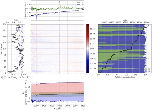
CTA 102 is reconstructed with four components that explain 99.98 per cent of its variance (see Fig. 17). This source hosts a bright BLR component that dominates during the observed low emission states. The excess of residuals observed around the emission lines may indicate a variation of these features, including the Fe ii. Such behaviour has been reported in the past by several authors in other blazars (see e.g. León-Tavares et al. 2013; Chavushyan et al. 2020; Hallum et al. 2020, for 3C 454.3, CTA 102, and 4C 29.45, respectively). Almost all the variability is associated with the second component (C2) due to its dominance during the flaring events detected, outshining the rest of the emission by two orders of magnitude. C2 is also the one showing the steepest slope (α = 1.2), while the component C4 has the hardest slope (α = 0.6). When the source is in low flux state, as the flux increases, the spectra show an RWB trend. During these periods, C3 and C4 are the dominant components. C3 contributes during short periods and for about 20 per cent to the mean flux, while C4 contributes more when the C2 is less important. For fluxes ≳ 10−14 erg cm−2 s−1 Å−1, C2 becomes dominant, and the colour trend is reversed, leading to a BWB one. This change is also visible in the overall colour variability of CTA 102 that shows a mild BWB evolution during the bright flare occurred between MJD 57400 and MJD 58400.
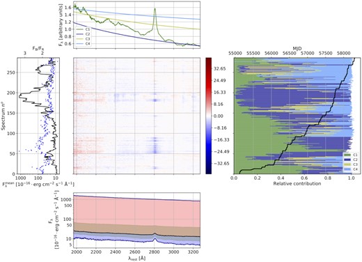
Results of CTA 102 (same description as Fig. 8).
5.3.5 3C 454.3
3C 454.3 is one of the most variable sources in the data sample, showing several flares with a flux increase of one order of magnitude. Its emission is also reconstructed with three components with an accuracy of ∼98.96 per cent. This reconstruction is shown in Fig. 18. The first one (C1) models the constant contribution of the BLR (it accounts for about 5 per cent of the |$\sigma ^2_{\rm exp}$|). The second (C2) and third (C3) components are PLs that account for the variable part of the emission, contributing with the 85 and 10 per cent of the |$\sigma ^2_{\rm exp}$|, respectively.
Results of 3C 454.3 (same description as Fig. 8).
The component C1 contributes with more than 80 per cent of the emission during the low states (the periods MJD 55500–56400 and 57800–57900) and only 10 per cent during high states. C2 is associated with prominent flares, e.g. at MJD 55250, 55500, and 56750. The component C3, a nearly flat PL, shows a large contribution in two periods around MJD 55100 and 56900. The residuals from the reconstruction show positive and negative excesses coincident with the Mg ii emission line, which may indicate variations in the line intensity, as reported by León-Tavares et al. (2013).
Overall, the source shows different colour trends with the flux variation. First, an RWB trend typically associated with the FSRQs is seen as the flux increases. A saturation in the colour appears at a flux level of ∼ 0.5 × 10⁻¹⁴ er g cm−2 s−1 Å−1, continuing with an mild BWB evolution, that is not commonly seen in FSRQs. This behaviour was first detected by Villata et al. (2006). Isler et al. (2017) also identified different trends by studying the optical/near-infrared (IR) emission and colour variations in 3C 279. The colour behaviour can also be related with the two reconstructed components associated with the jet. The third component shows an almost flat spectrum, being partly responsible for the observed RWB trend. Moreover, the second component is also responsible for the RWB behaviour below a certain flux value. For larger contributions of this component, the colour trend is reversed to account for the overall BWB tendency for the brightest spectra.
6 INTERPRETATION
6.1 Galaxy-dominated sources
Only three sources of the sample have found to be dominated by the galactic emission. The overall variability of these objects is significantly smaller than that from BL Lacs or FSRQs, as reflected by the low values of the fractional variability in the optical band. This is also shown in the right-hand panel of Fig. 19, where the explained variance scaled with the Fvar of the component associated with the jet is much lower than those of BL Lacs and FSRQs, where the jet is much more variable. As mentioned for Mkn 501, this is due to the fact that these objects are HSP BL Lac objects (see Section 5.1.1). The low variability of these blazars was reproduced using the stellar population plus the synchrotron emission of the jet. The host galaxy of these targets has a relative contribution of the 40–60 per cent to the total emission each source. Even though these objects show little intrinsic variability both in optical and γ-rays, our results show that the stellar population component (C1) remains almost constant, as expected (see Fig. 19). The variable component (C2) is a PL with spectral indices in the range of other BL Lac objects. Its variation is responsible for the observed BWB trends. These mild BWB trends found suggest that, despite the dominance and brightness of the host galaxy, the spectral evolution of the galaxy-dominated blazars is dominated by the variability of the relativistic jet as expected.
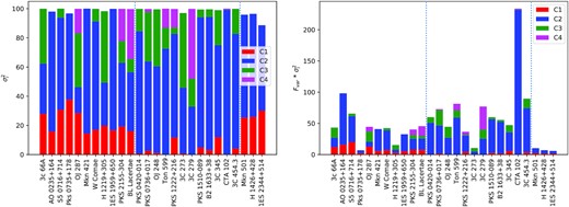
Explained variance of each component for all the data sample. Left-hand panel: total explained variance. Right-hand panel: explained variance scaled with the fractional variability. Vertical dotted lines separate the different types of blazars, classified according to their optical spectra: BL-Lac type at the left, FSRQs in the middle, and dominated by the host galaxy at the right.
6.2 BL Lac objects
The reconstruction of the optical spectra of BL Lac objects requires from two to four PLs, depending on the spectral variability exhibited by each object. Their indices range mostly from 0.5 to 1.9. This may be indicative of a jet with several emitting regions or substructures, that contribute differently to the emission. The variability in the emission of these regions could lead to both the flux variability and the spectral changes observed over time for these objects.
In some cases (e.g. 3C 66A), an extra component appears only for a limited period of time, that may be associated with a transient component in the jet. This behaviour can be caused by the injection of material or instabilities from the accretion disc to the jet, which can lead to the propagation of blobs, shocks, or instabilities through the jet, responsible for this emission (Marscher & Gear 1985; Marscher 2014). In this scenario, this component will only have a significant contribution to the emission of the source during a relatively short time interval.
The emission of BL Lacs is expected to have a radiatively inefficient accretion disc and a dominant jet characterized by synchrotron radiation (Fragile & Meier 2009). This scenario is completely consistent with our reconstruction of BL Lacs, in which all components are PLs associated with synchrotron processes. Most of the BL Lacs (8 out of the 11) studied here show a BWB behaviour in the colour variability. This can be understood in terms of our NMF decomposition by looking at the spectral indices of the components. By construction, C1 is taken to be at a low or quiet state of the source, whereas C2 and the other components that are added to account for the variable term. Our results indicate a prevalence of flatter slopes in the C1 component with respect to the others, which tend to show steeper slopes (see Table 2). For each object the component with the steepest slope coincides with the one explaining the most of the variance. Thus, it is clear that when the flux increases the spectrum becomes bluer. Li et al. (2015) claim that chromatic variations may be produced by shock-in-jet mechanisms in flares, while achromatic variability, such as the flare of OJ 287, may be due to geometrical effects. Additionally, the low brightness of their accretion disc is consistent with our reconstruction, where all the components are associated with the synchrotron emission of the jet. This behaviour is likely a result of a less efficient cooling and a very faint accretion disc (Isler et al. 2017).
6.3 FSRQs
As observed in Fig. 1, these are typically the most variable AGNs of the sample. FSRQs are reproduced with the BLR contribution plus two PLs. In some cases another PL is required, giving a total of four different contributions. The PL indices are similar to those found in BL Lacs, although the median value is slightly higher. Some of the FSRQs of the sample display steep and less variable components in their reconstruction: 3C 273, PKS 0736+017, PKS 1222+216, PKS 1510−089, and B2 1633+38 (see Fig. 20). This may be associated with the existence of a bright accretion disc emitting in the UV regime, and extending to optical wavelengths. The slow and low amplitude variation expected from an accretion disc matches the low variability displayed by these components. Moreover, the presence of an enhanced disc was already reported by Raiteri et al. (2014) in the modelling of the optical-IR SEDs of B2 1633+38, PKS 1510−089, and 3C 273. Additionally, some sources also display some low amplitude and slow varying trend in the BLR component. This slow varying trend observed in the BLR component can be associated with the variability of the accretion disc coupled with the broad line emission, and the time-scales of these trends are compatible with the slow variability of the accretion disc.
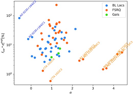
Explained variance scaled with the fractional variability for each component versus the corresponding spectral index.
The colour variability of these sources does not generally follow a unique RWB behaviour historically as associated with FSRQs, but shows different trends. Isler et al. (2017) explains this with the presence of an accretion disc and the different relative contributions of this thermal emission and the non-thermal synchrotron radiation coming from the jet. They identify different regimes that explain the different trends in the colour variability:
If the jet is in a quiescent state, the accretion disc can be observed in optical to UV wavelengths. In the optical/near-IR regime, the contribution of the disc is bluer, and thus, the spectra tend to bluer colour values. Therefore, as the non-thermal synchrotron contribution increases, it causes a reddening of the spectra as the emission of the jet equals the one from the disc (e.g. B2 1633+38; see Fig. 4).
Once the jet overcomes the accretion disc, the colour variability flattens, leading to an approximately achromatic flux increase. This effect of ‘colour saturation’ has already been detected in the past in several FSRQs (see e.g. Villata et al. 2006; Fan et al. 2018b). An example of this can be observed for CTA 102 (see Fig. 4).
Finally, when the non-thermal emission from the jet fully outshines the thermal contribution from the disc, the colour is determined by the jet. There are two possible behaviours: BWB likely due to the synchrontron electrons reaching higher energies before the radiative cooling (e.g. 3C 454.3; see Fig. 4); or RWB if the electrons do not reach such high energies.
7 CONCLUSIONS
NMF is a powerful statistical tool that allows us to reproduce the variability observed in large spectral data sets with high accuracy. We have used an a priori knowledge of the expected emission of blazars to model and reproduce their emission in terms of a small number of components. The simplest cases correspond to those objects whose spectra are dominated by the stellar population of the host galaxy. In these cases the spectral variability is explained in terms of the constant contribution of the host galaxy plus a PL component accounting for the synchrotron emission of the jet that is responsible for the variability observed in these sources. BL Lacs are reconstructed with two to four PL components that account for the spectral variability of the relativistic jet. Furthermore, a QSO-like component is added to analyse FSRQs due to the presence of a bright BLR responsible for the broad emission lines that appear in their optical spectrum, and possibly the contribution of a bright accretion disc.
We have investigated the temporal evolution of the components intervening in the reconstruction of the spectral set of each object. This can result in the identification of transient components that can be associated with blobs or shocks propagating along the jet. Moreover, behaviours such as different colour trends can also be associated with some of the resulting components, revealing different physical processes (see Isler et al. 2017). Overall, almost all BL Lacs have found to be BWB (except for OJ 287, whose behaviour may be ruled by a supermassive binary black hole system; and AO 0235+164, that despite being a BL Lac, has some FSRQ-like characteristics, indicating that this blazar may be a transitional object). On the other hand, FSRQs typically display more complicated colour behaviours, with an RWB evolution for low flux states, a colour saturation, and in some cases a final BWB trend for the brightest states.
Some of the sources display a rather steep and low variable PL component in their reconstruction (see e.g. the case of 3C 273). These components can be a signature of an enhanced blackbody associated with a bright accretion disc. The slow and small variability associated with these components is compatible with the behaviour of an accretion disc, and the steepness of the spectra is naturally associated with the optical extension of the UV emission coming from the disc. The sources in which this behaviour was observed are also compatible with those needing an enhanced accretion disc for the optical-IR SED modelling performed by Raiteri et al. (2014). The different colour trends can help to make constrains on the brightness of the accretion discs of FSRQs.
We propose that an NMF analysis of larger spectral data sets will help to understand the origin of the variability observed in blazars and disentangle the relevant contributions to their emission. In this context, extending the analysis to the IR and UV domains can aid to disentangle the different components present in AGNs and be of great use to study the physical processes taking place in such extreme and violent objects. Moreover, radio data can have a crucial importance in detecting several components propagating through the jet, or substructures such as blobs, shocks, or instabilities. Extending this methodology to other AGN types can also shed light in the evolution and unification of AGNs.
SUPPORTING INFORMATION
Figure A1. Results of H 1426+428 (same description as Fig. 8, available in the online version).
Figure A2. Results of 1ES 2344+514 (same description as Fig. 8, available in the online version).
Figure A3. Results of PKS 0735+178 (same description as Fig. 8, available in the online version).
Figure A4. Results of W Comae (same description as Fig. 8, available in the online version).
Figure A5. Results of H 1219+305 (same description as Fig. 8, available in the online version).
Figure A6. Results of 1ES 1959+650 (same description as Fig. 8, available in the online version).
Figure A7. Results of PKS 2155−304 (same description as Fig. 8, available in the online version).
Figure A8. Results of BL Lacertae (same description as Fig. 8, available in the online version).
Figure A9. Results of PKS 0420−014 (same description as Fig. 8, available in the online version).
Figure A10. Results of PKS 0736+017 (same description as Fig. 8, available in the online version).
Figure A11. Results of OJ 248 (same description as Fig. 8, available in the online version).
Figure A12. Results of Ton 599 (same description as Fig. 8, available in the online version).
Figure A13. Results of PKS 1510−089 (same description as Fig. 8, available in the online version).
Figure A14. Results of B2 1633+38 (same description as Fig. 8, available in the online version).
Figure A15. Results of 3C 345 (same description as Fig. 8, available in the online version).
Please note: Oxford University Press is not responsible for the content or functionality of any supporting materials supplied by the authors. Any queries (other than missing material) should be directed to the corresponding author for the article.
ACKNOWLEDGEMENTS
JOS acknowledges the support from grant FPI-SO (Ayuda de Formacion de Personal Investigador Severo Ochoa) from the Spanish Ministry of Economy and Competitiveness (MINECO)(research project SEV-2015-0548-17-3 and predoctoral contract BES-2017-082171).
JOS, JAP and JBG acknowledge financial support from the Spanish Ministry of Science and Innovation (MICINN) through the Spanish State Research Agency, under Severo Ochoa Program 2020-2023 (CEX2019-000920-S) and the project PID2019-107988GBC22.
OGM acknowledges financial support from the project [IN105720] DGAPA PAPIIT from UNAM.
Data from the Steward Observatory spectropolarimetric monitoring project were used. This program is supported by Fermi Guest Investigator grants NNX08AW56G, NNX09AU10G, NNX12AO93G, and NNX15AU81G.
We thank the anonymous referee for his/her comments that helped to improve the manuscript.
DATA AVAILABILITY
The data underlying this paper are available in Steward Observatory Database, at http://james.as.arizona.edu/~psmith/Fermi/DATA/specdata.html.
Footnotes
The NASA/IPAC Extragalactic Database (NED) is operated by the Jet Propulsion Laboratory, California Institute of Technology under contract with the National Aeronautics and Space Administration.
REFERENCES
APPENDIX A: REMARKS ON INDIVIDUAL SOURCES
Here we describe the results of the NMF analyses for the rest of blazars not presented in Section 5. The figures are available in the online version of this paper.
A1 Galaxy-dominated sources
H 1426+428
Similarly to 1ES 2344+514 and Mkn 501, this blazar emission displays a bright stellar emission that contributes with approximately 30 per cent of the total optical emission detected and shows little variability (|$F_{\rm var}\simeq 9{{\ \rm per\ cent}}$|). The results of this reconstruction are displayed in Fig. A1. The second component, associated with the jet, accounts for the rest of the emission and the low variability observed on this blazar. The spectral shape on H 1426+428 remains roughly constant during the monitoring due to its low variability. Thus, the colour of this source does not show large variations or correlation with the flux.
1ES 2344+514
The optical spectral variability of this blazar is very low (|$F_{\rm var}\simeq 4{{\ \rm per\ cent}}$|). 1ES 2344+514 has a bright host galaxy that contributes with 40–60 per cent of the optical emission of this source. The rest of the emission is associated with the jet, represented by the second component of the reconstruction. Fig. A2 displays the results of the reconstruction of this blazar. Despite its very small variability, it shows a mild overall BWB behaviour that comes from the component C2, associated with the jet, which has a not very steep slope. The colour trend is explained by the variable contribution of this component relative to the stellar population one.
A2 BL Lac objects
PKS 0735+178
The mean flux of the spectra shows very little variation (|$F_{\rm var}=7{{\ \rm per\ cent}}$|). The source is well reconstructed by two PL-like components C1 and C2, with spectral indices 0.63 and 1.45, respectively. Fig. A3 shows the results of the reconstruction of this source. The first component is always the brightest one. Its contribution to the mean flux is always above 80 per cent, and its mean flux remains nearly constant over time. It also displays a constant behaviour with respect to the colour. The largest flux contribution of the component C2 is about 20 per cent. Despite its low contribution, it accounts for more than half of the |$\sigma ^2_{\rm exp}$|. Moreover, the second PL shows a BWB behaviour and it explains the observed overall BWB trend, despite the low number of spectra. This BWB trend has also been observed in the past for this object (Meng et al. 2018).
W Comae
The variability of the BL Lac object W Comae is reproduced using three components associated with the synchrotron emission of the relativistic jet. These components are able to model the 99.86 per cent of the variability of this blazar. The results of this blazar can be seen in Fig. A4. The component C1 is the dominant when the mean flux is low. Its contribution to the |$\sigma ^2_{\rm exp}$| is around 20 per cent. The component C2 is the steepest one and its contribution to the |$\sigma ^2_{\rm exp}$| is above 70 per cent. It is the dominant component when the source is at high state. C3 is showing an almost flat slope (α = 0.18). It remains rather constant according to its contribution to the |$\sigma ^2_{\rm exp}$|, around 10 per cent. It shows a large contribution after MJD 56750, generally associated with low states, and it coincides with a reddening of the spectra. As for almost all the objects of its type, a long-term BWB evolution is observed for this object and it can be attributed to the variations of the component C2.
H 1219+305
Overall the spectra of H 1219+305 displays a relatively small variability (|$F_{\rm var}\sim 15\, {{\ \rm per\ cent}}$|). The flux of this blazar remains approximately stable during the whole observing period, although the colour FB/FR varies considerably in two epochs: from bluer in the period MJD 54800–54950 to redder in the period MJD 55200–55350. This BL Lac is reconstructed with three PL components, whose indices range from 0.72 to 1.26. The results of the NMF analysis are displayed in Fig. A5. The components C1 (α = 0.91) and C2 (α = 1.26) contribute almost equally to the mean flux during the first epoch when the spectra are bluer. The component C3 (α = 0.72) is dominant during the second epoch, when the spectra become redder. Since the average flux of the source remains nearly constant, no (anti)correlated trend with the colour is observed.
1ES 1959+650
The reconstruction of the spectra of this source is achieved with two components (see Fig. A6): The component C1 is rather stable (|$\sim 15{{\ \rm per\ cent}}\, \sigma ^2_{\rm exp}$|) and the component C2 is the one responsible of most of the variability. C1 resembles a rather flat PL, which also contains very faint absorption (Mg b) and emission ([O iii]5007 Å) features. Its contribution to the spectrum flux is almost unique when the target is at low state and moderate (|$\sim 50{{\ \rm per\ cent}}$|) at intermediate states. C2 is a blue PL that becomes very dominant when the source is on flare states. This object exhibits the typical BWB trend observed in BL Lacs. This behaviour was previously observed for this blazar (see e.g. Meng et al. 2018).
PKS 2155−304
A total of -four PL components were used to model the variability of the BL Lac object PKS 2155−304 (see Fig. A7). This reconstruction accounts for the 99.85 per cent of the variance of the original spectra. The component C1 contributes to the mean flux with 30–50 per cent of the emission for about 3/4 of the spectra, accounting for about 20 per cent of the |$\sigma ^2_{\rm exp}$|. The component C2 has its largest contribution associated with short flares, as shown by its higher contribution (40 per cent) to the |$\sigma ^2_{\rm exp}$|. C3 shows a contribution |$\gtrsim 60\, {{\ \rm per\ cent}}$| to the emission during the period MJD 56400–56600, being the main component when the colour is bluest. The component C4 is the less steep one. It contributes appreciably for short periods, being the main component when the colour is the reddest. A BWB trend is observed in the long-term variability of this blazar.
BL Lacertae
BL Lacertae was reconstructed using four PL components due to the high spectral variability displayed. The reconstruction accounts for the 99.71 per cent of the variance of the data set, and it is shown in Fig. A8. The PL indices range from 0.05 to 0.7. The component C1 shows a relatively flat slope (α = 0.27). Its spectrum also exhibits weak emission lines such as the H i recombination lines and [OIII]5007 Å. It has a moderate contribution, |$\lesssim 50{{\ \rm per\ cent}}$| to the total flux during the lower states, and accounts for |$\sim 15{{\ \rm per\ cent}}$| of the |$\sigma ^2_{\rm exp}.$| The components C2 and C4 are the most variable ones, being responsible for |$\sim 40{{\ \rm per\ cent}}$| and |$\sim 35{{\ \rm per\ cent}}$| of the |$\sigma ^2_{\rm exp}$|, respectively. Their slopes are very similar and may represent the evolution of the same physical component. The component C3 is almost flat and remains basically constant (|$10{{\ \rm per\ cent}}\, \sigma ^2_{\rm exp}$|). Its contribution to the total flux is as large as 60 per cent, not coincident with the high states. The overall evolution of this object follows the traditional BWB behaviour observed in BL Lacs, explained by the variable contribution of the blue components C2 and C4 (α ∼ 0.7), and expected from this dominant synchrotron emission.
A3 FSRQs
PKS 0420−014
The variability of PKS 0420−014 is accurately reproduced with three different components. The results are displayed in Fig. A9. The percentage of variance explained by the reconstruction of this target is 99.82 per cent. Despite its low time coverage, PKS 0420−014 is one of the few FSRQ showing the different trends reported by Isler et al. (2017). During its low flux state, it displays a very clear RWB evolution. At a flux of ∼10−15 er g cm−2 s−1 Å−1, this trend flattens, and the source starts becoming bluer as it brightens. The reddening evolution with increasing flux was reported in the past by Rani et al. (2010). However, the authors do not claim for the BWB trend that is also observed in this work.
The component C1 of the reconstruction (showing a prominent Mg ii line) is associated with the BLR. As expected, the variability associated with this component is very low (less than 1 per cent). Its contribution to the total flux is about 20 per cent most of the time, except for the period MJD 55300–55650. The components C2 and C3 account for the non-thermal synchrotron emission emerging from the jet. The component C2 is bluer, with a slope around 1.0 and it accounts for |$\sim 85{{\ \rm per\ cent}}$| of the |$\sigma ^2_{\rm exp}$|, becoming dominant in flux during high states. The component C3 is flatter and accounts for less than |$15{{\ \rm per\ cent}} \sigma ^2_{\rm exp}$|, but it contributes about 80 per cent of the flux when the source is at intermediate states. Each one is responsible of one of the two colour trends observed in PKS 0420−014. C2 accounts for the BWB trends during the flaring states. Furthermore, the component C3 explains the RWB trend.
PKS 0736+017
PKS 0736+017 is reconstructed with four components that explain 99.72 per cent of the variance of the data set. The results derived for this FSRQ are shown in Fig. A10. The first component, associated with the BLR, dominates up to a flux of ∼10−15 er g cm−2 s−1 Å−1. For brighter spectra, the jet components overcome the BLR emission. The component C1 contributes almost 80 per cent in most of the spectra, although accounts only for a very small fraction of |$\sigma ^2_{\rm exp}$|. The component C2 is the one accounting for most of the |$\sigma ^2_{\rm exp}$|, and its contribution to the mean flux reaches 70 per cent in coincidence with bright flares. The component C3 has the less steep slope, appearing during short periods associated with less intense flares. The component C4 has a very steep slope and appears only in about 10 per cent of the spectra, generally when the source is at low state. It accounts for a tiny fraction of |$\sigma ^2_{\rm exp}$|, indicating a rather small variability. This low variability and its steep PL are compatible with being the optical extension of the UV disc emission (similarly to the cases of 3C 273, PKS 1222+216, or B2 1633+38). Overall, the low state of the source does not reveal any clear colour trend. However, for the brightest spectra, a hint of the colour saturation already seen in other FSRQs is observed.
OJ 248
The reconstruction of OJ 248 was performed with a total of three components. This reconstruction is shown in Fig. A11. The BLR component observed in this FSRQ is always outshined by the PL components associated with the relativistic jet, and contributes with ∼25 per cent of the optical emission, except during the enhanced state observed at MJD 56300. Despite its low contribution to |$\sigma ^2_{\rm exp}$|, the mean flux of component C1 shows a slow monotonic increase of about 20 per cent in around 10 yr. The component C2 (α = 1.33) is dominant in about half of the spectra, especially when the colour of the source is the bluest. The component C3 (α = 1.06) contributes about 80 per cent to the mean flux, and its maximum coincides when the colour is the reddest, just before the big flare at MJD 56250. The low emission state of OJ 248 does not reveal any clear spectral evolution, with no trend between the colour and the flux, and large colour variation when the flux remains roughly constant, which coincides with an increase of the relative contribution of C1 at MJD ∼57800. A RWB trend is observed for OJ 248 during the low states between MJD 54700 and MJD 56250, approximately. Moreover, an FWB brightening is detected for the outburst observed during the flaring event at MJD 56300. The rising of the PL components is responsible for the FWB. Additionally, a very mild BWB increase is observed during the increase experienced at MJD 57750.
Ton 599
The spectra of this blazar show a broad line emission that is typically weaker than the emission of the jet. The reconstruction of the spectra was done using four components (see Fig. A12). The component C1 corresponds to the BLR emission. It shows a strong emission line corresponding to Mg ii 2800 Å, plus a fainter [OII]3727 Å. This component contributes at most by |$\sim 50{{\ \rm per\ cent}}$| to the mean flux during low states and remains basically constant. The component C2 contributes up to 50 per cent when the source is at high states and carries out most of the |$\sigma ^2_{\rm exp}$|, around 75 per cent. The components C3 and C4 show the most and the less steep slopes (α = 1.7, 0.9), respectively. They contribute more within the periods when the colour becomes bluer (component C3) and redder (component C4), in both cases with contributions above 25 per cent for |$\sim 30{{\ \rm per\ cent}}$| of the whole spectrum set. As it happened to other FSRQs, for the brightest spectra, a colour saturation, followed by an achromatic brightening, can be seen for this blazar.
PKS 1510−089
The NMF reconstruction of PKS 1510−089 is obtained using three components. The results of the NMF analysis performed on this object can be seen in Fig. A13. PKS 1510−089 displays a bright BLR represented by the first component of the reconstruction. This is the dominant contribution for about 80 per cent of the spectra, except for three short outburst events at MJD 55000, MJD 57150, and MJD 57600, respectively. As expected, the BLR contribution is approximately constant, and no trends or correlations are seen with the colour. The second component is a simple PL accounting for the emission of the jet and 91 per cent of the |$\sigma ^2_{\rm exp}$|. It is usually less bright than the BLR, except for the outbursts already mentioned. The contribution of this component varies correlated with the colour, displaying an RWB trend. This result is consistent with the one presented by D’Ammando et al. (2009), and follows the general behaviour of FSRQs. Overall, this blazar displays the classical RWB trend observed in FSRQs, and the colour saturation already discussed in other sources. Moreover, the component C3 shows a blue contribution, less bright than the BLR and the PL from the jet. It appears at low states of the source, shows little variation, and has a steep slope. These characteristics are compatible with the disc emission, which has been already suggested by Raiteri et al. (2014).
B2 1633+38
The spectra of this source have been reconstructed using three components (see Fig. A14): the first one represents the disc and BLR emission (showing the C [iv] and C [iii] features) that dominates up to a flux of ∼0.6 × 10⁻¹⁵ er g cm−2 s−1 Å−1. The second and third ones are PLs, with indices α = 1.2 and 2.3, respectively. The main contribution to the mean flux comes from the component C1, except when flares appear in which component C2 takes over, or component C3 in the period between MJD 56250 and 56400. The mean flux of C1 varies smoothly in scales of hundreds of days. Moreover, most of the variability (92 per cent of |$\sigma ^2_{\rm exp}$|) is due to the component C2. As it happened for 3C 273, the steep and less variable (|$\sigma ^{2}_{\rm exp} \simeq 5{{\ \rm per\ cent}}$|) component C3 may be associated with an enhanced blackbody explaining the contribution of the accretion disc. This would be in agreement with the need for a bright accretion disc in the optical-IR SED modelling claimed by Raiteri et al. (2014). A loose RWB trend is observed for most of the spectra, except for the high flux regime, in which a flattening in the colour is seen (see Fig 4). This flattening coincides with the period when the component C2 is highest. A flattening in the colour-flux trend is also observed for the most intense spectra, sign of the colour saturation.
3C 345
The spectra of 3C 345 can be reconstructed using three components. The results can be seen in Fig. A15. 3C 345 has an almost constant contribution |$\sigma ^{2}_{\rm exp} \simeq 10{{\ \rm per\ cent}}$| from the BLR that outshines the other two components used to explain the variability in this source for almost all the data set. This component has a constant contribution to the emission. It shows a relative contribution to the mean flux above 50 per cent for about 4/5 of the spectra. The mean flux associated with this component shows a clear slow decline trend, which may indicate a disc emission real variation. It does not show variations associated with changes in the colour of the source. The second and third components correspond to PL functions. The component C2 has a steep index (α = 1.72) and accounts for about 55 per cent of |$\sigma ^2_{\rm exp}$|. It contributes by about 60 per cent of the mean flux in the period around MJD 55100. The component C3 has a less steep index and accounts for about 30 per cent of |$\sigma ^2_{\rm exp}$|. It contributes with 30–40 per cent of the mean flux during the periods around MJD 55150 and 55300. The residual excess observed around the Mg ii emission line might indicate a variation of the line. A clear RWB colour evolution is show by this object, which can be explained by the increase of C2 and C3 relative to C1, which is slightly bluer. Apart from this trend, a flattening of the RWB trend is observed, leading to an almost achromatic variability when the source is in a high emission state.
