


ABSTRACT
We present photometric light curves of the stellar occultation event of the star UCAC4 341-187633 on 2018 August 15 by the minor planet (134340) Pluto. Photometric observations were carried out using the 2.1-m telescope at the San Pedro Mártir Observatory and the 1.3-m telescopes at Sites 2 and 3 of the Trans-Neptunian Automated Occultation Survey (TAOS II) project, and using a portable 0.4-m telescope from Bahía Asunción, Baja California Sur, Mexico. Different filters were used with the 2.1-m telescope and the TAOS II telescopes, whilst observations with the portable system were performed with no filter. The resulting light curves from the San Pedro Mártir Observatory show clear structures, with at least two bright spikes observed on ingress and one more observed on egress as the star traverses the atmosphere of the dwarf planet. The light curve from the portable telescope (440 km away) measured a longer duration for the occultation event, because the shadow of Pluto was observed at a lower latitude. Normalized light curves were created for the 2.1-m telescope, the Site 3 telescope of the TAOS II and the portable telescope. These normalized light curves show a difference in amplitude.
1 INTRODUCTION
For minor bodies in the Solar system, stellar occultations provide the most accurate means of determining their sizes, shapes and astrometric positions, which can be obtained from ground-based observations. A stellar occultation occurs when a body of the Solar system crosses the line of sight to a star, causing a variation in the apparent stellar brightness. From the features found in the brightness variations, the properties of minor bodies, such as size and shape, can be determined. Stellar occultations also offer the possibility to study atmospheric characteristics and planetary rings when these exist (Killian & Dalton 1985; Sicardy et al. 2020).
Pluto’s atmosphere was inferred from observations of occultation events starting in the late 1980s, particularly that of 1988 June 9 (Hubbard et al. 1988; Elliot et al. 1989; Millis et al. 1993). Since then, high signal-to-noise (S/N) light curves from stellar occultations have been used to determine and model Pluto’s properties, such as temperature, density and pressure profiles (Olkin et al. 2014; Dias-Oliveira et al. 2015; Gulbis et al. 2015; Sicardy et al. 2016; Meza et al. 2019, among others). An important feature detected in the occultation light curves reported by Hubbard et al. (1988) was the abrupt change in slope of the light curve of the event (called a ‘kink’ in some works). Elliot et al. (1989) proposed that such kinks could be due to the presence of an atmospheric haze layer and/or a thermal inversion. The presence of haze in the atmosphere of Pluto has been proposed to fit models to the data in other stellar occultation events as well (Elliot & Young 1992; Elliot et al. 2003; Olkin et al. 2014; Gulbis et al. 2015). In almost all of the light curves with high S/N, a change in slope is evident. Typically, this change is detected at approximately half of the amplitude of the light curve (half-light radius) and it is used to separate Pluto’s atmosphere into upper and lower parts, which are analysed separately in some studies. In addition to variations in the slope, some light curves also exhibit strong fluctuations (bright spikes), presumably resulting from local density perturbations, which can focus the star’s rays (e.g. Sicardy et al. 2003; Zalucha et al. 2007; Young et al. 2008b; Hubbard et al. 2009).
In the literature, almost 30 Pluto occultation events have been reported as successfully observed before the 2018 August 15 event. Meza et al. (2019) provides a list of 20 events, nine of which were observed at least in two different filter bands; however, of these nine events, only six observations were done at the same place using the same telescope or adjacent telescopes. Another event that is not listed in Meza et al. (2019), which was also observed using multiple filter bands, was carried out on 2007 July 31 (Young et al. 2008a; Olkin et al. 2014). The first of these multifilter events, which occurred on 2002 August 21, shows a clear dependence on wavelength, where the minimum flux is higher as the wavelength increases (Elliot et al. 2003). In a more recent stellar occultation event by Pluto in 2015 June, the same flux and wavelength dependence was observed by Person et al. (2021). Elliot et al. (2003) established that this dependence on wavelength should be expected to arise from the extinction caused by submicrometre-sized particles. This dependence might help to discern between thermal profiles and haze layers. In the case of Pluto’s atmosphere, the haze was originally proposed because this wavelength dependence was observed and later confirmed by observations from the New Horizons spacecraft (Cheng et al. 2017). Person et al. (2021) highlighted that the minimum flux of the light curves has never reached a value of zero for any observed Pluto occultation to date, indicating that at least a small amount of stellar flux is observable and implying that no Pluto occultation has yet extended down to reach the surface. It is worth mentioning that not all the stellar occultation events by Pluto observed at multiple wavelengths have detected a different relation between flux and wavelength.
In this paper, we present the results of our high-cadence photometric observations of the stellar occultation by Pluto of the event of 2018 August 15, from the San Pedro Mártir Observatory (OAN-SPM) using different filters, and also observations without any filter from Baja California Sur, Mexico. In Section 2 we describe the methodology used in the observations, in Section 3 we cover the data processing, and in Section 4 we discuss the data analysis. In Section 5, we present our discussion and conclusions.
2 OBSERVATIONAL DATA
We participated in an international campaign for observations of the stellar occultation event of the star UCAC4 341-187633 by (134340) Pluto, which occurred on 2018 August 15. The predicted maximum duration of the event was ∼126 s, and the shadow was predicted to cross the Earth in ∼8 min at a central time of ∼05:33:10 ut.1
We used three telescopes located at OAN-SPM: the 2.1-m telescope and two of the three 1.3-m Transneptunian Automated Occultation Survey (TAOS II) telescopes (Sites 2 and 3). We also used a portable telescope, which was set up close to Bahía Asunción, Baja California Sur, Mexico, about 440 km to the south of the OAN-SPM. Information about the observing campaigns is listed in Table 1.
Nominal characteristics of the telescopes used in this work.
| Site | Coordinates | Telescope | Camera | Diameter | Focal | Plate scale | Altitude | Filter/passband | |
|---|---|---|---|---|---|---|---|---|---|
| Longitude | Latitude | design | (m) | length | (arcmin mm−1) | (m) | |||
| OAN-SPM | −115.463689 | 31.044130 | Ritchey-Chrétien | Andor Ixon | 2.12 | f/7.5 | 13.0 | 2800 | i-Gunn system |
| Central 820 nm | |||||||||
| Width 130 nm | |||||||||
| OAN-SPM | −115.455322 | 31.041301 | Site 2 Cassegrain | CIS 107 | 1.3 | f/4 | 39.3 | 2820 | Short-pass |
| 400–710 nm | |||||||||
| OAN-SPM | −115.453938 | 31.041526 | Site 3 Cassegrain | Andor Zyla | 1.3 | f/4 | 39.3 | 2830 | Short-pass |
| 400–710 nm | |||||||||
| Bahía Asunción | −114.2806883 | 27.164932 | Ritchey-Chrétien | QHY 174M | 0.4 | f/9 | 60.24 | 50 | No filter |
2.1 Observations with the 2.1-m telescope
The 2.1-m telescope was equipped with an Andor iXon Ultra 888 EMCCD camera (hereafter, iXon), which was operated in frame transfer acquisition mode at a readout cadence of ∼10 Hz. With an array of 1024 × 1024 13-|$\rm{\mu m}$| pixels, this camera covered a field of view (FoV) of ∼2.9 × 2.9 arcmin2 (see Fig. 1a). A Gunn system i-band filter and 2 × 2 binning were used. The time for the shadow’s centre to cross over the OAN-SPM zone was expected to be a few seconds after 05:32:00 ut. We observed for approximately 1 h, starting at ∼05:00 ut, collecting a total of 36 000 images. An important characteristic of the Andor iXon camera (and the Andor Zyla used at Site 3 of TAOS II) is the accuracy in the kinetic cycle time (KCT;2,3 i.e. the time between the start and finish of each kinetic scan, which is needed to know the acquisition rate of the camera). This was also considered by Souza et al. (2006) who selected the Andor iXon DU-897 camera model to develop an occultation event observation system (POETS – the Portable Occultation, Eclipse and Transit System). Souza et al. (2006) analysed the characteristics of full-frame, interline-transfer and frame-transfer camera models, finding the frame-transfer model to be their best choice. However, the precision of the time recorded in the image header is no better than 1 s. Because these cameras generate data fits-cubes, only the beginning of the observation is stamped in the header, and then the total exposure time is calculated using the KCT. Souza et al. (2006) use an TM-4 GPS timing system from Spectrum Instruments, Inc., to determinate the beginning of the observations in the POETS. In our case, to improve the accuracy in the time estimation, we used the Astro Flash Timer cell-phone application a total of three times, to flash out the primary mirror during the observation. The Astro Flash Timer cell-phone application is recommended by the International Occultation Timing Association.4 Some tests were carried out with two cell-phone models (Iphone 6s Plus and Iphone 5), to measure the precision in time for flashes; this resulted in 1–7 ms for the Iphone 6 Plus model, while for the Iphone 5 it resulted in 9–15 ms.5 For our observations, we used an Iphone 6s model, an intermediate model between 5 and 6s Plus models, which can provide a precision better than 15 ms. Network effects in phone clocks cannot be quantified, so we decided to adopt a more conservative error, of the same order as the integration time (i.e. 0.1 s). The three flashes were registered at 05:03:00.795, 05:23:00.806 and 05:45:00.799 ut, each with a duration of 0.2 s. The flashes were evident in image numbers 1426–1427, 12908–12910 and 25538–25540, respectively. We subsequently calculated the approximate time for the beginning of the observations to be 05:00:31.9 ± 0.1 s ut and the centre of the event to be at ∼05:32:11 ut, in accordance with the predicted time. We calculated a precise observing cadence of 0.10452 ± 0.00002 s (∼9.56 Hz, in agreement with the KCT in the header from iXon) with an integration time of 0.1 s.
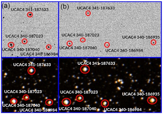
Field of view from the cameras used: (a) Andor iXon from the 2.1-m telescope; (b) a portion of QHY from the 40-cm telescope. Top panels: images obtained from the cameras. Bottom panels: images obtained from the Aladin Lite site (https://aladin.u-strasbg.fr).
2.2 TAOS II observations
The three telescopes of the TAOS II project (Lehner et al. 2018) in San Pedro Mártir have primary mirrors of 1.3 m in diameter and plate scales of f/4 (∼39.3 arcsec mm−1).
The observations from Site 2 were performed with the TAOS II prototype camera (hereafter, CIS107), which is equipped with an e2v CIS107 CMOS imager (Wang et al. 2014). From a total of 19 000 pixels available, we used a region of interest (ROI) of 90 × 90 pixels. Each pixel has a size of 7 |$\rm{\mu m}$|, resulting in a FoV of ∼25 × 25 arcsec2 for the selected ROI. We observed for ∼1.5 h with a cadence of ∼20 Hz, using a short-pass filter with transmission wavelength between 400 and 710 nm (64–598 from Edmund Optics).
At Site 3, we used an Andor Zyla 5.5sCMOS camera (hereafter, Zyla). The CMOS sensor in the camera has an array of 2160 × 2560 pixels of 6.5 |$\rm{\mu m}$|, and an ROI of 512 × 512 and 2 × 2 binning were used. The camera coupled to the telescope resulted in a FoV of |$\sim 2.2\, \times \,$|2.2 arcmin2 for the selected region. We observed for ∼40 min, also with a cadence of ∼20 Hz. For this camera, the KCT is 0.050056 s, for an integration time of 0.05 s, resulting in a dead time of 0.000056 s, and we used a filter identical to that used at Site 2. The timing information for the CIS107 and Zyla images was incorrect as the TAOS II site was under development at the time of the observations and the network installation was not yet complete. Thus, we used the spikes in the light curves (see Figs 3 and 6) to fit the time by comparison to the iXon data. Sites 2 and 3 of TAOS II are separated by less than 130 m, while Site 2 and the 2.1-m telescope are separated by approximately 850 m. The difference in height between telescopes is less than 40 m. The apparent velocity of Pluto’s shadow at the moment of the stellar occultation event was ∼19.3 km s−1; considering our estimated error in observation time of 0.1 s, this is equivalent to ∼1.9 km. The distance among telescopes is smaller than the error, so we consider it is valid to use the spikes in the light curves to adjust the time.
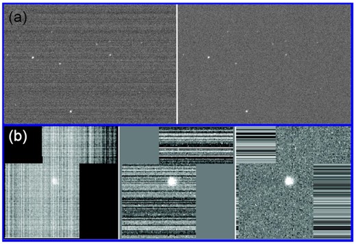
Images before and after the sigma clipping process for the (a) QHY and (b) CIS107 images.
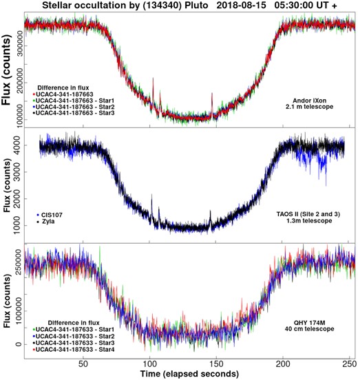
Light curves for the iXon, Zyla, CIS107 and QHY data obtained from the photometric process using iraf. Top: single photometry for UCAC4 341-187633 and differential photometry for iXon data (difference between occulted star and comparison stars is shown in the same scale as those of the single photometry). Middle: light curves from CIS107 and Zyla data (CIS107 shown at scale to Zyla). Bottom: single and differential photometry for QHY data. Comparison stars UCAC4 340-187040, UCAC4 340-187023, UCAC4 340-186984 and UCAC 340-186935 correspond to Star1, 2, 3 and 4 respectively.
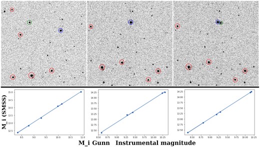
Example of a linear fit to the iXon data. Upper panels: images of the previous night (left), during the stellar occultation event (centre) and after the occultation event (right). The stars used for calibration are circled in red, Pluto is shown in green and the occulted star in blue. Lower panels: linear fits to the i-Gunn instrumental magnitude versus i-SMSS magnitude.
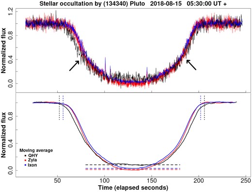
Top: comparison of the iXon, QHY and Zyla light curves (normalized flux). Arrows indicate kinks in the measured light curves. Bottom: moving average for the same light curves. QHY light curve results from the difference in flux of the occulted star (i.e. average of comparison stars 2 and 3), while the iXon and Zyla light curves result just from the occulted star. For the normalization, Pluto’s flux is used as a minimum while a sum of fluxes from Pluto and the star was used as a maximum. The number of points used in the moving average are 60 for QHY, 150 for iXon and 300 for Zyla, corresponding to approximately 15 s. The moving average light curve for the QHY camera was shifted 3 s to the right for a better visualization with respect to the other light curves. The horizontal lines indicate the level of amplitude of the curves, and the vertical lines indicate the approximate beginning and end of the event.
![Central region of flattened light curves (LCF) for the iXon and Zyla cameras. The light curves were flattened with: LCF = [1 − (normalized light curve − moving average)]. Three large spikes are clearly evident, and less intense spikes seen simultaneously in both light curves are indicated by arrows.](https://oup.silverchair-cdn.com/oup/backfile/Content_public/Journal/mnras/511/4/10.1093_mnras_stac401/1/m_stac401fig6.jpeg?Expires=1750481451&Signature=npaLG3sTcecEQBtqQL4BN10GglvcsgBNbugWIa-VeBoeKAZYLYrNXhrW-P~yjmGcvmWPuMO5tdQBlqE9tpc-xMUD95qNADLrj4dLnTFCUcHY9fNQbm~lHpEgASGTiekvvxs4mKchE-bLk0hg2jGoCHcwjaOju3Bk-SM6cycHLJSY-2dihJM647RWWz-mcP9CZkBasukQw~BjV6JJHOUVNmoclOw2uLz1TkG4txLKZOxDvWRTyzV8Mrv~WmcfLrE~A69i8VhCrdhBy2DyYTAg0htKFUilbaiCQbGm7Zy9ZHcn5CXmQfJ-dFRd~hTFnqq8w7kn0ua8bEMEjUkQUyoHAA__&Key-Pair-Id=APKAIE5G5CRDK6RD3PGA)
Central region of flattened light curves (LCF) for the iXon and Zyla cameras. The light curves were flattened with: LCF = [1 − (normalized light curve − moving average)]. Three large spikes are clearly evident, and less intense spikes seen simultaneously in both light curves are indicated by arrows.
2.3 40-cm telescope observations
Observations from Bahía Asunción, Baja California Sur, Mexico (lat. 27.164932, long. 114.280688333; closer to the central event chord in comparison to the OAN-SPM) were carried out with a QHY 174M camera (hereafter, QHY). The QHY has an array of 1920 × 1200 5.85-|$\rm{\mu m}$| pixels, giving a FoV of |$\sim 11\, \times \,$|7 arcmin (Fig. 1b). We observed with this system for ∼40 min using a readout cadence of 4 Hz, and no filter was used. The time stamps in the headers, set using a GPS, have precision better than 0.1 s.
3 DATA PROCESSING
Image processing was performed using the multitask software iraf.6 The science images were processed using flat and bias calibration images when available (flat and bias for the iXon and QHY cameras, and for CIS107 just bias). Because of the low integration time, the average number of counts for the dark frames were similar to the bias frame, so dark frames were not used. We used the zerocombine, flatcombine and ccdproc tasks to clean the images. A sigma clipping process using Python libraries was performed for the QHY images to eliminate a pattern in the columns (see Fig. 2a) and in the Zyla images to eliminate row and column patterns (see Fig. 2b). The sigma clipping process helped us to produce less noisy light curves, while the maximum and minimum levels are unchanged in comparison with the light curves calculated without the sigma clipping process. Aperture photometry for the occulted star and comparison stars (when available) was carried out with the qphot task while trying to follow the standard rule of using 2–3|$\, \times \,$|FWHM for the apertures (Harris & Warner 2006; Howell 2006). Finally, to achieve the highest S/N ratio, apertures with radii of 8, 5, 8 and 3 pixels were used for the iXon, Zyla, CIS107 and QHY images, respectively. The sky coordinates and visual magnitude for the occulted star UCAC4 341-187633 and comparison stars are listed in Table 2.
Right ascension, declination and visual magnitude for occulted and comparison stars.
| ID | RA (J2000.0) | Dec. (J2000.0) | MV |
|---|---|---|---|
| UCAC4 341-187633 | 19 22 10.5 | −21 58 49 | 13.1 |
| UCAC4 340-187040 | 19 22 14.4 | −22 00 22 | 12.6 |
| UCAC4 340-187023 | 19 22 11.6 | −22 00 10 | 14.2 |
| UCAC4 340-186984 | 19 22 06.3 | −22 00 25 | 13.9 |
| UCAC4 340-186935 | 19 21 56.3 | −22 00 17 | 12.8 |
For the iXon data, three comparison stars (see Fig. 1a) were used to calculate differential photometry. The light curves obtained (from single and differential photometry) are shown in Fig. 3. We can see in the top panel in Fig. 3 that all curves are similar. No comparison stars were available in the observations performed with the CIS107 and Zyla cameras due to the small RoIs. The respective light curves from these cameras are shown in the middle panel of Fig. 3. Because of the larger observation cadence and smaller telescope aperture, the S/N ratios of the light curves from the Zyla and CIS107 data are lower in comparison to that of the iXon light curve.
The CIS107 and Zyla light curves are similar in amplitude and dispersion, but the CIS107 light curve appears to be noisier at the end of the egress. The TAOS II telescopes were in the commissioning phase at this point, and there was no guiding system in place. The target star drifted across the ROI during the observations, and the noise at the end of the event is likely caused by non-uniform photometric response in the pixels in the prototype imager. Because of this noise excess, we used only the Zyla light curve from TAOS II for comparison purposes in this paper. The amplitude for the Zyla and iXon light curves is different, but we ascribe this to the fact that we are using different filters. We discuss this effect in the next section. Four comparison stars were used in the QHY data to calculate differential photometry, and three of these are the same stars used with the iXon data (see Fig. 1). Although we use a longer integration time, the S/N ratio is not as good because of the smaller telescope aperture and less favourable photometric conditions at the site. The light curves obtained are shown in the bottom panel of Fig. 3. The error in photometry is less than 0.01 mag for all data sets.
3.1 Normalized light curves
Using the iXon camera at the 2.1-m telescope, we were able to observe UCAC4 341-187633 the night before the occultation event, as well as ∼3.5 h after the occultation, when the occulted star and Pluto were visibly separated. We observed at a cadence of 10 Hz using an i-Gunn filter. We processed 2000 images from the previous night, 2000 images after the occultation event and six field stars (four in common between the two data sets) to calculate approximate absolute magnitude for Pluto. The data used to calibrate the magnitude were taken from the SkyMapper Southern Sky Survey7 (SMSS; Onken et al. 2019), and the i magnitude for the stars used is listed in Table 3. The i filters from the SMSS and the Gunn system are slightly different, but the objective of this comparison was to evaluate the behaviour of Pluto’s flux and not to determine its absolute magnitude. With the instrumental i magnitude and SMSS magnitudes, we calculated the linear correlation of the magnitudes and used it to correct the magnitudes of Pluto and the occulted star. The difference in the average magnitude for the occulted star was 0.006 mag. while for Pluto it was 0.015 mag. An example of the images and the linear fits used to correct the absolute i magnitude are given in Fig. 4. The error in the i Skymapper magnitudes of the stars used is less than 0.005 mag. As no transformation equation is involved, the error in the determination of this approximate corrected magnitude should be of the order of the error in the photometry (i.e. less than 0.01 mag).
Stars used to calculate calibrated absolute magnitudes, with the imagnitude taken from the SMSS. An asterisk denotes stars used in iXon images.
| ID | RA (J2000.0) | Dec. (J2000.0) | Mi | ErrMi |
|---|---|---|---|---|
| J192210.46−215848.9 | 290.544 | −21.980 | 12.8249 | 0.004* |
| J192214.42−220021.8 | 290.560 | −22.006 | 12.3829 | 0.004* |
| J192211.54−220010.7 | 290.548 | −22.003 | 13.3213 | 0.004* |
| J192206.28−220025.1 | 290.526 | −22.007 | 13.202 | 0.004* |
| J192217.10−220026.5 | 290.571 | −22.007 | 14.092 | 0.004* |
| J192217.59−215810.0 | 290.573 | −21.969 | 15.0164 | 0.004* |
| J192207.66−220043.7 | 290.532 | −22.012 | 14.2107 | 0.005* |
| J192216.25−215900.1 | 290.568 | −21.983 | 14.2443 | 0.004* |
| J192156.27−220016.7 | 290.484 | −22.005 | 11.7673 | 0.006 |
| J192153.87−215838.5 | 290.474 | −21.977 | 13.2629 | 0.005 |
| J192153.00−215950.8 | 290.471 | −21.997 | 13.1761 | 0.004 |
| J192226.31−215613.4 | 290.610 | −21.937 | 12.7027 | 0.004 |
| J192230.01−215644.6 | 290.625 | −21.946 | 13.0911 | 0.004 |
| J192227.98−220036.7 | 290.617 | −22.010 | 11.4831 | 0.006 |
Pluto’s rotational period is ∼153 h,8 and our data sets have a difference of approximately 24 h in time, meaning that Pluto rotated about |$15{{\ \rm per\ cent}}$| of its rotational period over the course of the observations. Buratti et al. (2003) measured an amplitude of less than 0.3 mag (R-Johnson filter), and the minimum time for this amplitude from their light curves was ∼50 h. We can thus expect that Pluto’s brightness did not significantly change throughout our observations.
We used the corrected magnitudes of Pluto calculated from the observations after the occultation event to determine FP, and we used the corrected magnitude of the occulted star during the event to calculate F. We used 450 images (equivalent to approximately 45 s) before ingress and 450 images after egress to calculate FSP. This FSP was similar to the combined flux of Pluto and the occulted star before and after the event: FSP/(F + FS)before ∼ FSP/(F + FS)after ≈ 0.998.The normalized light curve from the iXon data is shown in Fig. 5.
For the QHY camera, observations were obtained the night previous to the stellar occultation event. The observations were made with an integration time of 1 s and 2 × 2 binning. We carried out imilar process to that of the iXon data, but in this case we used 12 stars in the field with i-SMSS magnitudes (see Table 3) to calculate the trend and correct the magnitude for the occulted star. From this magnitude, we calculated the average flux of the unocculted target star FS. For the observations of the occultation night, nine stars were used to correct the magnitude of the occulted star. From this corrected magnitude, we calculated the flux F. An average magnitude value was calculated using 180 images (equivalent to approximately ∼ 45 s) before the ingress and 180 images after egress, and this value was used to calculated FSP. We used the difference in flux for FSP and FS to determinate the flux of Pluto’s FP. The normalized light curve from the QHY data is shown in Fig. 5.
For the Zyla camera, we used images acquired more than 3 h after the stellar occultation event, when the star and Pluto were visibly separated. We determined the median values of the flux for Pluto (FP) and the occulted star (FS). The sum of these values is similar to the median value of FSP, considering 1000 images (equivalent to approximately ∼50 s) taken before the ingress and 1000 images after egress, with FSP/(FP + FS) ≈ 0.999. We thus used the value FSP = FS + FP. It should be noted that the results were similar when mean values were used instead of medians. The normalized light curve from the Zyla data is shown in the upper panel of Fig. 5.
For CIS107 data, no observations before or after the occultation event were acquired, so for that reason no normalized light curve was calculated.
4 DATA ANALYSIS
In the top panel of Fig. 5, we overlayed the three normalized light curves obtained in this work from the iXon, Zyla and QHY cameras. In the bottom panel of Fig. 5, we show the corresponding moving averages of the same light curves from the top panels. For the iXon and Zyla light curves, the beginning and the end of the occultation event occurred approximately at 05:30:56 and 05:33:22 ut, respectively (values 56 and 202 on the x-axis in Fig. 5), for an event duration of approximately 146 s. A slight change in the slope during the ingress part of the light curve occurred at ∼05:31:20 ut (elapsed time of 80 s). During the egress, a slightly more pronounced change in the slope occurred at ∼05:33:00 ut (elapsed time of 180 s) approximately at the same height in the normalized flux. This change is more evident for Zyla and iXon images, showing an asymmetry at the lower part of the curve.
For the QHY light curve observed from Bahía Asunción, the beginning of the event occurred approximately at 05:30:51 ut, and the end was approximately at 05:33:23 ut, close to the same times as the iXon and Zyla light curves. The occultation duration time of approximately 152 s is longer than that measured at the OAN-SPM, given that the observations occurred closer to the equator of the projected shadow. The changes in the slopes of the curves are different for iXon, Zyla and CIS107, being more steep in ingress and less evident in egress (but more tilted), at ∼05:31:14 and 05:33:26 ut, respectively. The asymmetry in the QHY light curve is evident. In the first part of the curve (ingress), the change is less prominent in comparison with the iXon and Zyla curves, but the second part (egress) is very similar. However, it is difficult to determine if this asymmetry is due to an intrinsic characteristic of the event or due to the larger noise in the light curve. A difference in amplitudes between the three light curves is also evident (here, amplitude is defined as the difference in normalized flux, between the base level, which corresponds to the value of 1.0, and the bottom of the light curve), being greater in the curve obtained with the Zyla camera. The light curve for QHY has the lowest amplitude, but the bottom of this light curve is more noisy, masking possible characteristics, such as spikes, and making it difficult to determinate the amplitude of the light curve with more precision. To better estimate the amplitudes, we thus performed a moving average on the normalized flux for each of the light curves (see the bottom panel of Fig. 5). From these averaged light curves, we determined amplitudes (using the median value of the central region) of 0.918, 0.991 and 0.968 for QHY, Zyla and iXon, respectively.
Elliot et al. (2003) postulated that the measured differences in amplitudes from different telescopes for the 2002 August 21 event were due to the fact that the telescopes observed with filters over a wide range of passbands. This is expected to be caused by extinction from small (<1 |$\rm{\mu m}$|) particles in Pluto’s atmosphere.
Fig. 6 shows the central region of flattened light curves for the iXon and Zyla cameras. At least two bright spikes are observed on ingress and one more is observed on egress as the light from the star traverses Pluto’s atmosphere. Each of these events is clearly resolved, containing several data points. Other structures with lower heights can also be clearly seen in each light curve. Zalucha et al. (2007) established that because of the wavelength dependence of atmospheric refractivity, longer wavelength light is expected to arrive at larger distances from the centre of the occultation event. However, because the refraction spikes were used to synchronize the Zyla and iXon data, no such analysis can be performed on this data set.
Synthetic light curves were obtained based on the atmospheric model developed by Dias-Oliveira et al. (2015, hereafter DO2015). In this model, we are considering a spherical transparent atmosphere made of N2 only, with no local pressure variations or haze. We discarded the high-frequency variations in the data (spikes and other features) by applying a lowpass Fourier filter, and then fitted the temperature profile around the values provided by DO2015, as well as the values of pressure for 1275 and 1215 km from the centre of the Dwarf Planet. For geometric purposes, we fitted the light curve from the 2.1-m telescope in the OAN-SPM and the light curve from our mobile 40-cm telescope in Bahía Asunción B.C.S., our southernmost station. As for the pressure estimation, our best fitting shows that for 1215 km it is 10.55 μbar, which corresponds to 3.57 μbar for 1275 km for the iXon data while for QHY data our best fittings were 7.9 μbar for 1215 km and 2.7 μbar for 1275 km. However, hereafter we refer to the pressure values obtained from the Ixon observations. DO2015 reported pressures at 1275 km of 2.16 and 2.3 μbar in 2012 and 2013, respectively. In 2019, Meza et al. (2019) reported 6.61 μbar at 1215 km for the occultation of 2016 and predicted a decrease in the atmospheric pressure around 2020. We report that, in 2018, there were significant increments of 35 per cent since 2013 (DO2015) and 37 per cent since 2016 (Meza et al. 2019). However, Arimatsu et al. (2020) reported a drop in pressure of 21 per cent (5.2 μbar at 1215 km) from observations obtained in 2019. Our results are consistent with the increasing trend of pressure observed up to 2015, and would indicate an event with a more abrupt pressure drop for the results of Arimatsu et al. (2020). Fig. 7 shows the fit between our observations and the model for iXon and QHY. We summarize the model parameters in Tables 4 and 5.
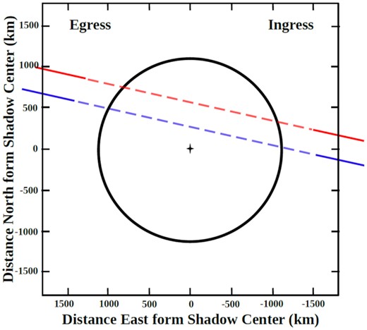
Pluto’s observation geometry from our light curves. Blue line show the chord’s path from Bahía Asunción while red line displays the chord path from OAN-SPM.
Pluto’s atmospheric model characteristics: physical parameters.
| Parameter | Value |
|---|---|
| Pluto’s mass (× G, m3s−2) | 8.703 × 10¹¹ |
| Nitrogen molecular mass (kg) | 4.652 × 10⁻²⁶ |
| Nitrogen molecular refractivity (cm3 molecule−1) | 1.091 × 10⁻²³ + [6.282 × 10⁻²⁶/(λ2)] |
| Boltzman constant (J K−1) | 1.380626 × 10⁻²³ |
| Central wavelength (μm) | iXon 0.77, QHY 0.5 |
Pluto’s atmospheric model characteristics: free parameters.
| iXon | QHY | |
| Critical temperature points at radii of: | ||
| 1190.4 km | 36.46 K | 35.76 K |
| 1217.3 km | 110.11 K | 111.79 K |
| 1302.4 km | 94.65 K | 97.59 K |
| 1392.0 km | 83.32 K | 76.0 K |
| Constants of the temperature profile (DO2015 model): | ||
| c1 | 1.42 × 10⁻⁶ | 1.41 × 10⁻⁶ |
| c2 | 2.5 × 10⁻³ | 2.6 × 10⁻³ |
| c3 | −2.2 × 10⁻⁹ | −2.2 × 10⁻⁹ |
| c4 | −4.84 × 10⁻¹³ | −4.78 × 10⁻¹³ |
| c5 | 8.67 × 10⁻⁸ | 8.67 × 10⁻⁸ |
| c6 | −36210 | −36210 |
| c7 | 8.27 × 10⁻² | 8.28 × 10⁻² |
| c8 | 4 − 6.27 × 10⁻⁸ | −6.27 × 10⁻⁸ |
| c9 | 1.58 × 10⁻¹⁴ | 1.58 × 10⁻¹⁴ |
| Pressure at: | ||
| 1275 km | 3.57 ± 0.001 μbar | 2.7 ± 0.1μbar |
| 1215 km | 10.55 ± 0.001 μbar | 7.9 ± 0.2μbar |
From the model, we calculated the length of the observed path (chords) for the iXon and QHY data. From these data we determined the geometry of the occultation. Fig. 8 shows the path where in Pluto’s shadow our chords were probed. The determined length for iXon data was about 2016 km, while QHY data a length of about 2191 km was estimated. The QHY chord has a less distance to the center of Pluto’s shadow in comparison to iXon data. The distances and their respective errors are listed in Table 6. Our results for adjusting the geometry are very marginal because we can only use two light curves.
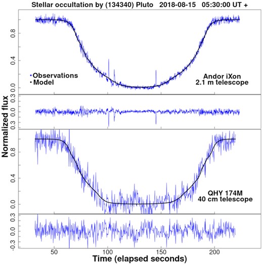
Fit between observations and the model calculated for atmospheric pressure determination.
Geometric parameters determined from the model.
| Chord radii | |
|---|---|
| iXon ingress | 1007.99 ± 0.15 km |
| iXon egress | 1008.20 ± 0.15 km |
| QHY ingress | 1096.99 ± 2.80 km |
| QHY egress | 1094.07 ± 2.80 km |
| Distance to Pluto’s shadow centre | |
| iXon chord | 735 ± 2.5 km |
| QHY chord | 539 ± 5.7 km |
| Chord radii | |
|---|---|
| iXon ingress | 1007.99 ± 0.15 km |
| iXon egress | 1008.20 ± 0.15 km |
| QHY ingress | 1096.99 ± 2.80 km |
| QHY egress | 1094.07 ± 2.80 km |
| Distance to Pluto’s shadow centre | |
| iXon chord | 735 ± 2.5 km |
| QHY chord | 539 ± 5.7 km |
5 DISCUSSION AND CONCLUSIONS
The main objective of this work is to present the observational data obtained from the stellar occultation event that occurred on 2018 August 15. We study how the characteristics of the light curves and how the observations obtained with different filters at two different locations (OAN-SPM and Bahía Asunción, B.C.S.) might contribute to obtain additional information about Pluto’s atmosphere.
The first stellar occultation by Pluto was observed in 1985 and reported by Brosch (1995). The quality of the acquired data at the time made a more detailed analysis of the atmosphere difficult. The second and third observed stellar occultation events by Pluto were observed in 1988 and 2002, respectively. From there, it was determined that Pluto’s atmosphere had expanded and its atmospheric pressure doubled (Elliot et al. 2003; Sicardy et al. 2003). In subsequent years, the atmosphere expansion continued, although at a much slower rate (Dias-Oliveira et al. 2015; Sicardy et al. 2016). With our analysis, we estimated an increment of the pressure from 2016 to 2018, but Arimatsu et al. (2020), using the atmospheric model from DO2015 and similar conditions, reported a decrement in 2019 July. Given the significantly different characteristics of the light curves from various events over these past 30 yr, arising from different atmospheric features and properties, we can confirm that Pluto’s atmosphere is indeed very active.
Regarding the different wavelength observations, we identified reports in the literature of seven events with this information: 2002 August 21; 2007 March 18, June 14 and July 31; 2011 June 23; 2013 May 04; and 2015 June 29. In the 2002 August 21 event, Elliot et al. (2003) found a dependence between the wavelength and the flux. One of the possible explanations for this was the presence of haze in Pluto’s atmosphere, whose existence was confirmed by the New Horizons spacecraft (Cheng et al. 2017). However, Elliot et al. (2003) mentioned that the change in flux observed in the 2002 August 21 event could also be due to the contribution of a redder star close to the occulted star. In 2007 March 18, Person et al. (2008) reported the results of the observations carried out at three different sites, separated by linear distances of less than 200 km each, in which they used different filters (r′, I and H, with effective wavelengths of 640, 790 and 1650 nm, respectively); however, the chords were affected by the atmosphere of Pluto, in the sense that the body of the planet did not occult the star (Pluto’s atmospheric graze). In addition, one of the curves is incomplete and another is very noisy, thus making it impossible to carry out an analysis like that of Elliot et al. (2003).
The observations of 2007 June 14 were used in the work of Meza et al. (2019) to model the evolution of Pluto’s atmosphere. These observations were carried out at Paranal, Chile, with the UT1 8.2-m telescope and the u′, g′ and i′ filters (see table A1 of Meza et al. 2019) but the light curves that they show appear to be flat (constant flux; see fig. 1 of Meza et al. 2019).
For the observations of 2007 July 31, Young et al. (2008a) used two filters with effective wavelengths of 510 and 760 nm. The occultation was observed at Mount John Observatory in New Zealand; with a visible central flash in the light curves, they established that there is no difference in the amplitude of the light curves. Olkin et al. (2014) made an analysis using the same light curves and concluded that the amplitude is similar, but they established, by means of central flash modelling, that the flux cannot be explained only by haze, but it can be explained by a combination of haze and a thermal gradient or by a thermal gradient only.
For the occultation of 2011 June 23, Person et al. (2013) analysed several light curves, including three from the Stratospheric Observatory for Infrared Astronomy (SOFIA), observed in the blue and red channels. These light curves do not show evidence of changes in amplitude, but they do present a kink, although less pronounced than that from the 1988 June 9 event. Gulbis et al. (2015) addressed the issue by using light curves of an atmospheric graze by Pluto, observed using NASA’s 3-m Infrared Telescope Facility (IRTF) on Mauna Kea, Hawaii. The observations were collected in wavelengths using the MIT Optical Rapid Imaging System (MORIS) with no filter, and low-resolution near-infrared spectra were collected using the spectrograph SpeX. Spikes were observed in the resulting light curves that differed in amplitude in different passbands, and Gulbis et al. (2015) proposed the existence of a haze as an explanation of this wavelength dependence.
Dias-Oliveira et al. (2015) presented light curves from observations performed at the San Pedro de Atacama Observatory in 2013 May 04, using the 0.5-m Caisey telescope and B, R and V filters. In their fig. 4, two of these light curves show a slight difference in amplitude, but they are noisy and it is difficult to determine if the differences are indeed real. On 2015 June 29, Pasachoff et al. (2017) were able to observe an occultation at the Mount John Observatory using the 61-cm Boller & Chivens telescope. They observed simultaneously in g′, r′ and i′ filters (central wavelengths of 474, 622 and 765 nm, respectively). The observation’s cadence is relatively low (more than 6 s of integration), making it difficult to perform an analysis like the one done for the 2013 May 04 event. However, for every filter, the bottom of the light curves looks similar, within the level of noise. Person et al. (2021) present observational data at various wavelengths observed with SOFIA for the 2015 June stellar occultation event, using the following instruments: High Speed Imaging Photometer for Occultations (HIPO), First Light Infrared Test Camera (FLITECAM) and the Focal Plane Imager (FPI+). The effective central wavelengths of their observations were 0.57 |$\mu$|m for HIPO-blue, 0.65 |$\mu$|m for FPI+ , 0.81 |$\mu$|m for HIPO-red and 1.8 |$\mu$|m for FLITECAM. Their observations show the same dependence of increasing minimum flux as the wavelength increases, perceived by Elliot et al. (2003) in the August 2002 event. In their fig. 10, Person et al. (2021) make a direct comparison with the results of Elliot et al. (2003).
Our normalized light curves show a difference in amplitude, for the iXon and Zyla data, and the same dependence in wavelength as for the 2002 August (Elliot et al. 2003) and 2015 June (Person et al. 2021) events; however, the amplitude is smaller in the QHY data. This difference could be a wavelength dependence due to the effect of the atmosphere of Pluto, but a more detailed analysis should be done.
The light curves presented here, more precisely those observed from the OAN-SPM, have among the best S/N ratios and the highest cadence observed for these types of events, offering a good possibility to constrain models of Pluto’s atmosphere and determine the values of density, pressure and temperature profile. Our observations also display very evident spikes, which can be used to model density waves.
SUPPORTING INFORMATION
iXon_NLC.dat
QHY_NLC.dat
Zyla_NLC.dat
Please note: Oxford University Press is not responsible for the content or functionality of any supporting materials supplied by the authors. Any queries (other than missing material) should be directed to the corresponding author for the article.
ACKNOWLEDGEMENTS
This work was supported in part by Academia Sinica and the Universidad Nacional Autónoma de México. We acknowledge support from the DGAPA-UNAM project IN107316 and CONACYT Project CB283800. Based upon observations carried out at the Observatorio Astronómico Nacional on the Sierra San Pedro Mártir (OAN-SPM), Baja California, Mexico.
DATA AVAILABILITY
The data underlying this article will be shared on reasonable request to the corresponding author. Normalized light curves underlying this article are available in its online supplementary material.
Footnotes
iraf was distributed by the National Optical Astronomy Observatory, which was managed by the Association of Universities for Research in Astronomy (AURA) under a cooperative agreement with the National Science Foundation.
DOI: 10.25914/5ce60d31ce759
