


ABSTRACT
We present a comprehensive study of the gas kinematics associated with density structures at different spatial scales in the filamentary infrared dark cloud, G034.43+00.24 (G34). This study makes use of the H13CO+ (1–0) molecular line data from the ALMA Three-millimeter Observations of Massive Star-forming regions (ATOMS) survey, which has spatial and velocity resolution of ∼0.04 pc and 0.2 km s−1, respectively. Several tens of dendrogram structures have been extracted in the position-position-velocity space of H13CO+, which include 21 small-scale leaves and 20 larger-scale branches. Overall, their gas motions are supersonic but they exhibit the interesting behaviour where leaves tend to be less dynamically supersonic than the branches. For the larger scale, branch structures, the observed velocity–size relation (i.e. velocity variation/dispersion versus size) are seen to follow the Larson scaling exponent while the smaller-scale, leaf structures show a systematic deviation and display a steeper slope. We argue that the origin of the observed kinematics of the branch structures is likely to be a combination of turbulence and gravity-driven ordered gas flows. In comparison, gravity-driven chaotic gas motion is likely at the level of small-scale leaf structures. The results presented in our previous paper and this current follow-up study suggest that the main driving mechanism for mass accretion/inflow observed in G34 varies at different spatial scales. We therefore conclude that a scale-dependent combined effect of turbulence and gravity is essential to explain the star-formation processes in G34.
1 INTRODUCTION
High-mass stars (M⋆ > 8 M⊙) play a crucial role in the evolution of galaxies. They dictate the energy budget of the host galaxy via powerful radiation, outflows, winds, and supernova events, and are responsible for the production and transfer of heavy elements to the surrounding interstellar medium (ISM). They also influence future star formation in their natal molecular clouds (e.g. Kennicutt 2005; Urquhart et al. 2013). High-mass star formation has therefore long been the subject of intense astrophysical research after the basic scenario of isolated, low-mass star formation was established in the late 1980s (e.g. Shu, Adams & Lizano 1987). However, understanding the processes involved is not easy owing to the several observational challenges, e.g. large distances, short lifespans, and formation in clustered environment. Several great efforts from both observations and numerical simulations (e.g. Zhang et al. 2009; Wang et al. 2011, 2014; Peretto et al. 2013; Beuther et al. 2018; Motte, Bontemps & Louvet 2018; Yuan et al. 2018; Vázquez-Semadeni et al. 2019; Padoan et al. 2020; Liu et al. 2022) focused on the physical processes of star formation on multiple scales from molecular clouds, through filaments and clumps, and finally down to cores. These studies have revealed that high-mass star formation is a multi-scale, hierarchical fragmentation process that occurs on almost all relevant scales of density structures.
Density structures at different scales are intrinsically connected both spatially and kinematically. Spatially, they are nested in the top-down manner where molecular clouds form on scales of several tens of parsecs with low-density molecular gas (n ≲ 102–3 cm−3), evolve to clumps on scales of several parsecs with higher densities, and finally are concentrated into pre and proto-stellar cores on scales of ∼0.01–0.1 pc with even higher-density gas. Kinematically, density structures at different scales are correlated through coherent motions. A pioneering work on turbulence in the ISM by Larson (1981) proposed a velocity–size scaling relation, δv ∝ Lγ with γ = 0.38. Subsequent studies have established the universality of this scaling relation in diverse environments where a value of γ = 0.5 is commonly seen (e.g. Solomon et al. 1987; Heyer & Brunt 2004). This suggests that the gas motions of the giant molecular clouds (GMCs), in general, can remain coherent over four orders of magnitude of scales from ∼100 to 0.1 pc. Recent unprecedented, multi-wavelength Herschel observations have revealed the prevalence of intermediate-scale filamentary structures within individual molecular clouds. With numerous detailed kinematic studies from the observational perspective (e.g. Hacar et al. 2013, 2018; González Lobos & Stutz 2019; Liu, Stutz & Yuan 2019; Álvarez-Gutiérrez et al. 2021), these structures have been found to be velocity coherent.
Moreover, these observable results have been successfully reproduced with dedicated simulations (e.g. Smith, Glover & Klessen 2014; Vázquez-Semadeni et al. 2019; Padoan et al. 2020; Lu et al. 2021). For instance, recent state-of-the-art numerical simulations (e.g. Padoan et al. 2020) modelled the cloud complexes with a web of filaments, each with a longitudinal velocity gradient related to the directional mass flow converging towards the web node, where high-mass young stellar objects are preferentially formed. One of the key predictions from their simulations is that the mass of the final star is determined not only by the small clump- or core-scale mass accretion but also by the larger-scale, filamentary mass inflow/accretion. In other words, the mass of the newly formed stars is strongly related to the multi-scale, coherently dynamical mass inflow/accretion (a manifestation of gas motions), which agrees well with the results from recent dedicated multi-scale kinematic observations (Zhang & Wang 2011; Peretto et al. 2013; Yuan et al. 2018; Liu et al. 2022). In recent years, excellent facilities like the Submillimeter Array (SMA) and the Atacama Large Millimeter/submillimeter Array (ALMA), have opened up the possibility of studying the kinematics of density structures in high-mass star formation regions across multiple scales from clouds down to seeds of star formation thereby giving tremendous impetus to the field of high-mass star formation.
The target of this work is the densest central region of the filamentary cloud, G034.43+00.24 (hereafter G34, Shepherd, Nürnberger & Bronfman 2004; Rathborne et al. 2005; Rathborne, Jackson & Simon 2006; Shepherd et al. 2007; Cortes et al. 2008; Liu et al. 2020a, 2022) which is shown in Fig. 1. Located at 3.7 ± 0.3 kpc (e.g. Rathborne et al. 2005; Tang et al. 2019; Liu et al. 2020a, 2022), G34 is a well-known high-mass star-forming, filamentary infrared dark cloud (IRDC) with the two massive protostellar clumps (i.e. MM1, and MM2 in Fig. 1) located at the centre. These protostellar clumps have masses of the order of few hundred solar masses, sizes ∼0.2–0.5 pc, and luminosities of ∼104 L⊙ which are typical for high-mass protostars. Along with the IRDC nature of G34, the massive and luminous characteristics of the two clumps reflect early stages of high-mass star formation.
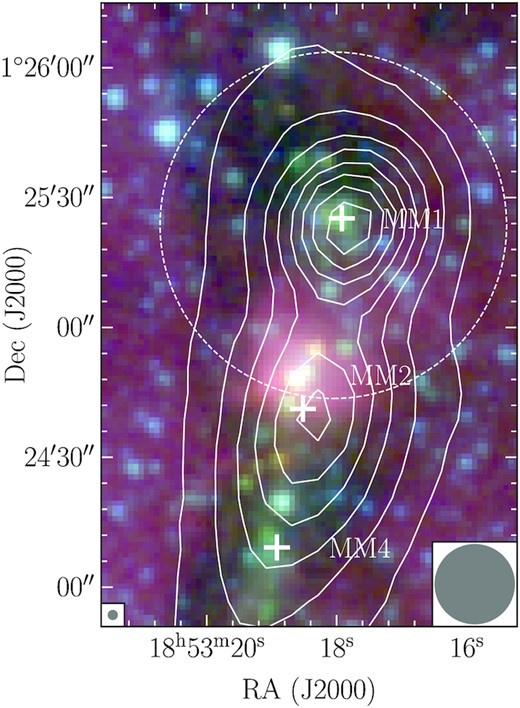
Overview of the densest central region of G34 harbouring a massive, high density structure with ongoing star formation that is probed by ATOMS (field of view indicated by the white dashed circle). Spitzer colour-composite image, 3.6 (blue), 4.5 (green), and 5.6 |$\mu$|m (red) is shown superimposed with the ATLASGAL 870 μm continuum contours. The contours start at 3 rms (rms ∼0.6 Jy beam−1) with increasing steps defined as the power-law D = 3 × Np + 2 with the dynamical range of the intensity map (i.e. the ratio between the peak and the rms noise) D, and the number of contours N (8 in this case). The region contains three massive protostellar clumps MM1, MM2, and MM4 cataloged in Rathborne et al. (2006). The field of view of the ATOMS observation covers the clump MM1 and part of clump MM2. The beams of the Spitzer and ATLASGAL data are shown at the bottom left-hand, and bottom right-hand corners, respectively.
In this paper, the third in the series of studies on IRDC G34 (Liu et al. 2020a, 2022, hereafter Paper I, and Paper II, respectively) and also a pilot study of multi-scale structures and kinematics using interferometric data from the ATOMS survey1 (Project ID: 2019.1.00685.S, Liu et al. 2020b, c, 2022, see Section 2), we aim to investigate the kinematics of density structures at different scales through the exemplary G34 cloud. In Paper I, we analysed in great detail the chemical components of nine protostellar clumps (i.e. MM1–MM9, see fig. 1 of Paper I) of G34, with observations of several ∼1 mm lines by the Atacama Pathfinder Experiment telescope. The study showed that the chemistry of the clumps is closely connected to their underlying physics related to star-formation activity (e.g. luminosity and outflows). Furthermore, fragmentation and dynamical mass accretion processes during the early stages have been revealed and assessed in great detail across multiple scales in Paper II. The analysis carried out in Paper I concluded that high-mass star formation in G34 could be proceeding through a dynamical mass inflow/accretion process linked to the multi-scale fragments from the clouds, through clumps and cores, down to seeds of star formation. In this work, we carry out a follow-up study of Paper II using the H13CO+ (1–0) line data. The sections are organized as follows: Section 2 briefly describes the ALMA-ATOMS data, Section 3 presents the dendrogram analysis of the H13CO+ (1–0) data including the identification of dendrogram structures, and their morphological and kinematic analysis, Section 4 discusses the cloud dynamical state, Section 5 gives its implication on star formation, and Section 6 summarizes the results.
2 ALMA DATA
The MM1 and MM2 clumps of G34 are covered in the observations of the target source I18507+0121 from the ATOMS survey. The detailed descriptions about the scientific goals of the survey, observing setups, and data reduction can be found in Liu et al. (2020b, c, 2021) and Paper II. In this paper, we only make use of the 12m+ACA combined data of H13CO+ (1–0). This line emission displays mostly single-peak profiles across the entire observed region (see Fig. A1). This is expected since the H13CO+ (1–0) line is generally considered to be relatively optically thin. In Paper II, we estimated the optical depth of this line towards the nine detected dense cores. The values were found to lie in the range of 0.04–0.39, thus supporting the above assumption for the G34 complex under study. This makes H13CO+ (1–0) emission line a good probe for tracing the kinematics and density structures at different scales of G34 without the complex effects from the optical depth and multiple velocity components. It is worth mentioning that H13CN (1–0), another optically thin molecular line, was also observed as part of the ATOMS survey. This dense gas tracer has hyperfine components where the isolated one has been used in literature to probe the gas kinematics. However, this isolated component is usually found to be too weak to trace extended emission as compared to H13CO+ (1–0) and hence not considered for the analysis presented in this work. Briefly, the combined data have a beam size of 1.9 arcsec × 2.1 arcsec, which corresponds to 0.04 pc at the distance of G34, and a sensitivity of ∼8 mJy beam−1 at a velocity resolution of 0.2 km s−1.
3 DENDROGRAM ANALYSIS OF H13CO+ (1-0)
3.1 Dendrogram structure identification
Dendrogram analysis was conducted to extract the density structures of different scales from the H13CO+ (1-0) data in a position-position-velocity (PPV) space using the Dendrogram algorithm.2 Following Rosolowsky et al. (2008), the dendrogram methodology works as a tree diagram that characterizes emission structures as a function of the level of three-dimensional intensity isocontours, and arranges them into a tree hierarchy composed of leaves and branches. In context of the tree hierarchy, the leaves are defined as the small scale, bright structures at the tips of the tree that do not breakup into further substructures. And branches are the larger-scale, fainter structures lower in the tree that do breakup into substructures.
In order to optimize the performance of the Dendrogram algorithm, noisy pixels, where the peak intensity along the spectral axis is less than five times the local noise level, were masked out to generate a modified data cube of H13CO+. Here, the local noise level was considered since the actual noise distribution is not uniform in the ATOMS data due to different primary beam responses across the observed region. The local noise was estimated for each pixel of the data cube by taking the standard deviation of intensity in the line-free velocity channels spanning 20 km s−1 in velocity. The masked area in the new cube of H13CO+ can be easily seen in the moment maps presented in Fig. 2.

Moment maps of H13CO+ adapted from Paper II. (a): velocity-integrated intensity map of H13CO+ (1–0) for the G34 region probed with the ATOMS survey The integrated velocity range is 12 km s−1 centred at the systemic velocity 57.6 km s−1. The contours with the associated numbers correspond to the leaf structures identified by the Dendrogram algorithm (see text). (b): moment 1 map of H13CO+ (1–0). The arrows A–D mark the directions of the observed velocity-coherent gradients. (c): velocity dispersion map of H13CO+ (1–0). In all panels, the map is displayed only at the positions where the peak intensity of the H13CO+ spectrum is ≥5 times the local noise. The beam size is shown at the bottom left-hand corner.
With the masked H13CO+ data cube, we computed the dendrogram tree. The three key parameters that are used as an input to the algorithm are (i) min_value =5σ for the significance of the intensity peak of individual structures, where σ (=3.2 mJy beam−1) is the typical noise of the modified, masked data cube. There is an improvement of more than a factor of 2 in σ of the masked data cube as compared to the original data cube; (ii) min_delta =2σ for the minimum difference between two peaks for them to be considered separate structures; and (iii) min_npix =N pixels as a minimum number of spatial-velocity pixels for a resolvable structure, where N was set to be five times the synthesized beam area (e.g. Duarte-Cabral et al. 2021). In total, the Dendrogram algorithm identifies several tens of structures. After discarding those that appear spurious structures near the edges, where the relative noise is higher, we finally retain 41 structures, that includes 21 leaves and 20 branches. The Dendrogram tree of these structures is presented in Fig. A2.
In Fig. 2a, the spatial distribution of the identified leaf structures is displayed on the H13CO+ (1–0) velocity-integrated intensity adapted from Paper II. It can be seen that these structures correspond to bright emission of H13CO+ (1–0) very well. Comparing with the 3 mm dust continuum emission, where nine cores were detected (see fig. 1 of Paper II), the H13CO+ emission reveals more small-scale structures (21 leaves). This difference can be understood since H13CO+ has much more extended emission than 3 mm continuum (see fig. 2a of Paper II). However, the leaf structures extracted from the H13CO+ data are not resolved as well as the 3 mm continuum cores even though both data have similar angular resolutions. For example, Leaf 4 contains three 3 mm continuum cores MM1-a/b/f identified in Paper II. All such associations between the leaves and 3 mm continuum cores are listed in the last column of Table 1. Note that the poorly-resolved leaf structures do not affect the analysis carried out.
Parameters of dendrogram structures.
| ID | RA | Dec. | maj × min axis | PA | L | Fp | Tkin | Vel. range | 〈Vlsr〉 | δV | 〈σ〉 | 〈σnt〉 | Assoc. |
|---|---|---|---|---|---|---|---|---|---|---|---|---|---|
| (J2000) | (J2000) | arcsec × arcsec | deg | pc | mJy beam−1 | K | km s−1 | km s−1 | km s−1 | km s−1 | km s−1 | ||
| Leaves | |||||||||||||
| 0 | 18:53:19.28 | +1:24:46.53 | 8.4 × 3.2 | 111.1 | 0.08 | 63.8 | 9.4 ± 7.5 | (59.57, 61.26) | 60.21 ± 0.06 | 0.35 ± 0.04 | 0.45 ± 0.02 | 0.45 ± 0.03 | |
| 1 | 18:53:18.64 | +1:26:01.19 | 6.3 × 4.3 | 201.4 | 0.08 | 130.5 | 17.7 ± 10.8 | (57.46, 60.63) | 58.98 ± 0.04 | 0.34 ± 0.03 | 0.84 ± 0.02 | 0.84 ± 0.02 | MM1-g |
| 2 | 18:53:18.30 | +1:24:47.29 | 7.6 × 3.7 | 113.4 | 0.08 | 65.8 | 22.3 ± 4.0 | (52.82, 54.09) | 53.46 ± 0.04 | 0.17 ± 0.03 | 0.39 ± 0.02 | 0.39 ± 0.02 | |
| 3 | 18:53:18.67 | +1:24:49.05 | 4.6 × 3.7 | 50.3 | 0.06 | 98.0 | 28.6 ± 3.0 | (53.46, 54.72) | 54.12 ± 0.06 | 0.15 ± 0.04 | 0.37 ± 0.03 | 0.36 ± 0.04 | MM2-a |
| 4 | 18:53:17.94 | +1:25:24.89 | 15.3 × 12.1 | 49.8 | 0.24 | 166.1 | 24.0 ± 3.0 | (54.30, 60.42) | 57.46 ± 0.02 | 0.60 ± 0.01 | 1.33 ± 0.01 | 1.33 ± 0.01 | MM1-a/b/f |
| 5 | 18:53:19.01 | +1:24:51.25 | 5.7 × 4.7 | 115.6 | 0.08 | 73.7 | 11.2 ± 8.2 | (54.72, 55.57) | 55.19 ± 0.04 | 0.10 ± 0.03 | 0.26 ± 0.03 | 0.25 ± 0.03 | |
| 6 | 18:53:19.72 | +1:25:08.80 | 16.8 × 6.1 | 101.5 | 0.18 | 103.5 | 17.7 ± 10.8 | (58.73, 61.05) | 59.82 ± 0.03 | 0.45 ± 0.02 | 0.66 ± 0.01 | 0.66 ± 0.01 | |
| 7 | 18:53:18.33 | +1:26:01.83 | 10.3 × 2.2 | 177.2 | 0.07 | 115.3 | 17.7 ± 10.8 | (55.14, 57.46) | 56.03 ± 0.05 | 0.37 ± 0.04 | 0.55 ± 0.02 | 0.55 ± 0.02 | |
| 8 | 18:53:18.55 | +1:25:18.86 | 21.2 × 4.3 | 120.5 | 0.17 | 163.0 | 12.9 ± 2.3 | (57.25, 59.36) | 58.32 ± 0.02 | 0.37 ± 0.01 | 0.58 ± 0.01 | 0.57 ± 0.01 | MM1-c/d/e |
| 9 | 18:53:19.30 | +1:25:30.52 | 6.7 × 5.0 | 148.8 | 0.09 | 85.5 | 3.6 ± 0.1 | (57.46, 58.52) | 57.90 ± 0.04 | 0.23 ± 0.03 | 0.32 ± 0.02 | 0.32 ± 0.02 | |
| 10 | 18:53:19.19 | +1:26:00.08 | 6.0 × 3.9 | 130.6 | 0.08 | 99.2 | 17.7 ± 10.8 | (57.46, 60.21) | 58.79 ± 0.09 | 0.51 ± 0.06 | 0.79 ± 0.04 | 0.79 ± 0.04 | |
| 11 | 18:53:18.56 | +1:24:46.39 | 12.9 × 7.2 | 163.3 | 0.17 | 243.6 | 22.1 ± 8.2 | (55.14, 58.52) | 56.82 ± 0.03 | 0.70 ± 0.02 | 0.94 ± 0.01 | 0.94 ± 0.01 | MM2-b |
| 12 | 18:53:18.72 | +1:25:04.50 | 12.8 × 7.6 | 104.8 | 0.17 | 176.7 | 15.2 ± 8.2 | (57.68, 58.73) | 58.23 ± 0.02 | 0.22 ± 0.02 | 0.32 ± 0.01 | 0.31 ± 0.01 | |
| 13 | 18:53:18.72 | +1:25:36.01 | 7.7 × 5.1 | 123.5 | 0.10 | 126.0 | 19.5 ± 3.6 | (57.89, 59.57) | 58.71 ± 0.04 | 0.27 ± 0.03 | 0.48 ± 0.02 | 0.47 ± 0.02 | |
| 14 | 18:53:17.67 | +1:25:42.93 | 5.6 × 3.8 | 113.5 | 0.07 | 64.5 | 17.7 ± 4.3 | (58.31, 59.36) | 58.87 ± 0.06 | 0.10 ± 0.04 | 0.30 ± 0.04 | 0.29 ± 0.04 | |
| 15 | 18:53:18.71 | +1:25:49.47 | 12.8 × 5.2 | 78.0 | 0.14 | 95.4 | 8.9 ± 5.4 | (57.68, 59.15) | 58.48 ± 0.04 | 0.32 ± 0.03 | 0.43 ± 0.02 | 0.42 ± 0.02 | |
| 16 | 18:53:18.79 | +1:24:53.16 | 6.4 × 4.5 | 200.2 | 0.09 | 226.4 | 18.8 ± 6.4 | (58.10, 59.36) | 58.67 ± 0.05 | 0.25 ± 0.04 | 0.40 ± 0.03 | 0.39 ± 0.03 | |
| 17 | 18:53:19.32 | +1:25:50.45 | 6.8 × 4.2 | 75.1 | 0.09 | 77.5 | 17.7 ± 10.8 | (57.89, 59.15) | 58.56 ± 0.05 | 0.13 ± 0.03 | 0.31 ± 0.03 | 0.31 ± 0.03 | |
| 18 | 18:53:19.76 | +1:25:14.62 | 9.2 × 3.0 | 174.7 | 0.08 | 79.2 | 17.7 ± 10.8 | (58.52, 59.57) | 58.95 ± 0.05 | 0.20 ± 0.04 | 0.30 ± 0.03 | 0.29 ± 0.03 | |
| 19 | 18:53:19.91 | +1:25:28.79 | 7.5 × 3.4 | 167.8 | 0.08 | 87.6 | 17.7 ± 10.8 | (57.89, 58.73) | 58.17 ± 0.07 | 0.22 ± 0.05 | 0.25 ± 0.03 | 0.24 ± 0.04 | |
| 20 | 18:53:19.19 | +1:24:55.81 | 7.5 × 4.2 | 67.9 | 0.09 | 162.8 | 17.7 ± 10.8 | (57.89, 58.94) | 58.41 ± 0.04 | 0.14 ± 0.03 | 0.34 ± 0.03 | 0.33 ± 0.03 | |
| Branches | |||||||||||||
| 21 | 18:53:18.51 | +1:25:10.72 | 78.5 × 29.2 | 86.9 | 0.85 | 243.6 | 18.2 ± 9.6 | (52.82, 61.89) | 57.65 ± 0.01 | 1.69 ± 0.01 | 1.42 ± 0.01 | 1.42 ± 0.01 | |
| 22 | 18:53:18.51 | +1:25:10.51 | 78.0 × 28.9 | 86.9 | 0.85 | 243.6 | 18.2 ± 9.6 | (52.82, 61.89) | 57.65 ± 0.01 | 1.72 ± 0.01 | 1.42 ± 0.01 | 1.42 ± 0.01 | |
| 23 | 18:53:19.73 | +1:25:09.85 | 19.3 × 6.9 | 102.6 | 0.20 | 103.5 | 17.7 ± 10.8 | (58.52, 61.05) | 59.75 ± 0.04 | 0.65 ± 0.03 | 0.70 ± 0.02 | 0.70 ± 0.02 | |
| 24 | 18:53:18.51 | +1:25:07.97 | 69.1 × 28.9 | 84.0 | 0.80 | 243.6 | 19.3 ± 8.3 | (53.25, 61.26) | 57.60 ± 0.01 | 1.52 ± 0.01 | 1.39 ± 0.01 | 1.39 ± 0.01 | |
| 25 | 18:53:18.46 | +1:25:07.38 | 69.5 × 24.8 | 83.7 | 0.74 | 243.6 | 19.2 ± 8.1 | (53.25, 61.05 ] | 57.55 ± 0.01 | 0.99 ± 0.01 | 1.35 ± 0.01 | 1.35 ± 0.01 | |
| 26 | 18:53:18.50 | +1:25:07.76 | 68.7 × 28.1 | 83.8 | 0.78 | 243.6 | 19.4 ± 8.3 | [ 53.25, 61.05) | 57.60 ± 0.01 | 1.42 ± 0.01 | 1.39 ± 0.01 | 1.38 ± 0.01 | |
| 27 | 18:53:18.51 | +1:25:11.41 | 79.7 × 29.5 | 87.5 | 0.86 | 243.6 | 18.2 ± 9.8 | (52.82, 62.53) | 57.65 ± 0.01 | 1.63 ± 0.01 | 1.42 ± 0.01 | 1.42 ± 0.01 | |
| 28 | 18:53:18.52 | +1:25:10.49 | 77.8 × 28.9 | 86.9 | 0.85 | 243.6 | 18.2 ± 9.6 | (53.25, 61.68) | 57.67 ± 0.01 | 1.54 ± 0.01 | 1.40 ± 0.01 | 1.40 ± 0.01 | |
| 29 | 18:53:18.51 | +1:25:07.83 | 68.8 × 28.6 | 84.1 | 0.79 | 243.6 | 19.3 ± 8.4 | (53.25, 61.05) | 57.60 ± 0.02 | 1.77 ± 0.01 | 1.39 ± 0.01 | 1.38 ± 0.01 | |
| 30 | 18:53:18.63 | +1:24:56.04 | 43.8 × 15.8 | 94.6 | 0.47 | 243.6 | 20.2 ± 9.9 | (54.72, 59.78) | 57.52 ± 0.01 | 0.96 ± 0.01 | 1.17 ± 0.01 | 1.17 ± 0.01 | |
| 31 | 18:53:18.46 | +1:25:05.87 | 62.4 × 20.9 | 81.9 | 0.64 | 243.6 | 20.8 ± 7.8 | (54.09, 60.42) | 57.54 ± 0.01 | 1.14 ± 0.01 | 1.27 ± 0.01 | 1.27 ± 0.01 | |
| 32 | 18:53:18.63 | +1:24:58.42 | 55.0 × 16.8 | 93.8 | 0.54 | 243.6 | 19.3 ± 9.6 | (54.72, 60.00) | 57.59 ± 0.01 | 0.98 ± 0.01 | 1.19 ± 0.01 | 1.19 ± 0.01 | |
| 33 | 18:53:18.65 | +1:24:52.77 | 31.8 × 15.3 | 102.8 | 0.39 | 243.6 | 24.2 ± 7.3 | (54.72, 59.78) | 57.49 ± 0.02 | 0.94 ± 0.01 | 1.15 ± 0.01 | 1.15 ± 0.01 | |
| 34 | 18:53:18.63 | +1:24:58.93 | 57.4 × 17.4 | 94.5 | 0.56 | 243.6 | 19.1 ± 10.0 | (54.72, 60.21) | 57.60 ± 0.01 | 1.11 ± 0.01 | 1.19 ± 0.01 | 1.19 ± 0.01 | |
| 35 | 18:53:18.62 | +1:24:52.00 | 30.2 × 11.3 | 100.2 | 0.33 | 243.6 | 24.0 ± 7.4 | (54.93, 59.57) | 57.42 ± 0.02 | 0.94 ± 0.02 | 1.12 ± 0.01 | 1.12 ± 0.01 | |
| 36 | 18:53:18.60 | +1:24:47.80 | 15.9 × 9.1 | 132.6 | 0.21 | 243.6 | 21.5 ± 8.6 | (55.14, 59.57) | 57.12 ± 0.04 | 1.05 ± 0.03 | 1.13 ± 0.01 | 1.13 ± 0.01 | |
| 37 | 18:53:18.66 | +1:25:55.49 | 22.3 × 8.2 | 74.7 | 0.24 | 130.5 | 5.4 ± 1.9 | (55.14, 61.68) | 58.70 ± 0.03 | 1.02 ± 0.02 | 1.03 ± 0.03 | 1.03 ± 0.03 | |
| 38 | 18:53:18.72 | +1:25:54.96 | 21.2 × 10.2 | 67.2 | 0.26 | 130.5 | 17.7 ± 10.8 | (55.14, 61.68) | 58.69 ± 0.03 | 1.13 ± 0.02 | 0.97 ± 0.02 | 0.96 ± 0.02 | |
| 39 | 18:53:18.70 | +1:25:54.59 | 23.1 × 6.0 | 81.3 | 0.21 | 130.5 | 11.4 ± 6.6 | (57.25, 60.84) | 58.61 ± 0.03 | 0.59 ± 0.02 | 0.66 ± 0.02 | 0.65 ± 0.02 | |
| 40 | 18:53:18.51 | +1:25:11.57 | 79.7 × 29.5 | 87.4 | 0.87 | 243.6 | 18.2 ± 9.8 | (52.82, 62.53) | 57.65 ± 0.01 | 1.79 ± 0.01 | 1.42 ± 0.01 | 1.42 ± 0.01 | |
Note. Notes. The size, L, is calculated as |$\sqrt{\rm maj. \times min.}/3600 \times \pi /180\times D$| given the distance D = 3.7 kpc of G34. The kinetic temperature of each structure, Tkin, and its uncertainty are derived from the NH3 kinematic temperature map taking the mean value and standard deviation, respectively, in the structure. The mean velocity of a structure, 〈Vlsr〉, is computed from the intensity-weighted first moment and the uncertainty of 〈Vlsr〉 from δVlsr/|$\sqrt{N}$| where N is the number of independent beams within the structure. The velocity variation of a structure, δVlsr, is inferred from the standard deviation of Vlsr in the structure and the uncertainty of δVlsr from |$\delta V_{\rm lsr}/\sqrt{2(N-1)}$|. The mean velocity dispersion of a structure, 〈σ〉 is given by the intensity-weighted second moment and the uncertainty of 〈σ〉 by 〈σ〉/|$\sqrt{N}$| with the number of independent beams within the structure N. The last column, Assoc., indicates the association between the leaves and dust continuum cores identified in Liu et al. (2022).
The measured parameters of all dendrogram structures are listed in Table 1. These include the coordinates, the major and minor axes, the position angle, the peak flux, and the velocity range in which the structures span. Note that the major and minor axes values listed in the table are corrected by a filling factor as described below. The original major and minor axes returned by the Dendrogram algorithm are the intensity-weighted second spatial moments along the two axes (Rosolowsky et al. 2008). Consequently, the calculated area of the ellipse (Aell) of each structure is much smaller than the exact area (Aext) of the structure in the plane of the sky. To alleviate this, we define a filling factor, |$\sqrt{A_{\rm ext}/A_{\rm ell}}$|, which is multiplied to the original major and minor axes. Accordingly, the final size of the structures can be estimated as the geometric mean of the corrected axes (Col. 6 of Table 1).
Next, the mean velocity 〈Vlsr〉 of the structures was computed from the intensity-weighted first moment map (see Fig. 2b) over their associated velocity span, the velocity variation δVlsr is estimated from the standard deviation of Vlsr in the structures, and the mean velocity dispersion 〈σ〉 is obtained from the intensity-weighted second moment (see Fig. 2c). The kinetic temperature Tkin of each structure was estimated from NH3 observations (at 3 arcsec resolution) toward G34 by Lu et al. (2014) and the non-thermal velocity dispersion was calculated as |$\sqrt{\langle \sigma \rangle ^2-\sigma ^2_{\rm th}}$|, where σth is the thermal component of the velocity dispersion (see equation 2 of Liu et al. 2019). Note that not all of the structures are recovered in the interferometric kinetic temperature map. For such structures, the Tkin values were assumed to be the mean value of the entire map. In addition, NH3 and H13CO+ may not trace the same gas even at these high spatial resolutions, and thus the NH3-based temperature should be treated with caution. All the above parameters are also listed in Table 1.
3.2 Dendrogram morphological analysis
Fig. 3 displays the histograms of size and axial ratio for the dendrogram structures. The size distribution of the leaves peaks at ∼0.07 pc with a median value of 0.09 pc within the range (0.06, 0.24) pc, while the branches peak at ∼0.80 pc, with a median value of 0.60 pc within (0.20, 0.87) pc. There is a marginal peak seen at ∼0.20 as well. It is interesting to note that size distribution of the leaves peaks at the minimum L value in contrast to the branches where the peak coincides with the maximum branch size. Overall, the typical size of the branches is greater than that of the leaves, which follows from the definition of these two different scale structures. Moreover, the axial ratio of the leaves show a more uniform and wider distribution with a median value of 0.59 within (0.20, 0.83), while the corresponding distribution of the branches peaks at ∼0.37 with a median value of 0.37 within (0.26, 0.57). The leaves appear, on average, more circular and are presumably more spherical compared to the branches. Additionally, it can be found from the H13CO+ emission map in Fig. 2 that the peak of the axial ratio distribution of the branches nearly matches the aspect ratio (∼0.35 pc) of the whole filamentary morphology of G34.

Histograms of leaf and branch properties: size (L), axial ratio, mean Vlsr (〈Vlsr〉), Vlsr variation (〈δV〉), mean velocity dispersion (〈σ〉).
3.3 Dendrogram kinematic analysis
The general kinematic properties of the dendrogram structures are shown in Fig. 3 in terms of 〈Vlsr〉, δVlsr, and 〈σ〉. For the mean velocity (〈Vlsr〉) distribution, the branches are concentrated around the peak at the median value ∼57.5 km s−1and lie within the narrow range (57.1, 59.4) km s−1. The peak corresponds to the systemic velocity (57.6 km s−1; Paper II) derived from the average spectrum of H13CO+ over the entire region investigated here. This means that majority of the branches constitute large-scale structures that contain kinematic information representative of the entire region. In contrast, the leaves display a wide range, (53.5, 60.2) km s−1, peaking at 58.5 km s−1 with a median value of 58.4 km s−1. This spread of the mean velocity for the leaves agrees with the non-uniform velocity field of G34 as shown in Fig. 2b.
Considering the velocity variation (δVlsr) distribution, we find the trend that the leaves (median 0.25 km s−1) are on average ∼4.5 times lower than the branches (median 1.12 km s−1). Larger δVlsr values for branches could be related to turbulence, gravity-driven motions, or large-scale ordered motions (see below). In particular, leaves 4 and 11 have δVlsr ≥ 0.6 km s−1, which fall in the overlap region with the branches. These two leaves are also among the larger ones. Here, localized outflows from star formation feedback, as revealed in Paper II, could be an additional source for these larger δVlsr values.
For the velocity dispersion (〈σ〉) distribution, the leaves peak at ∼0.35 km s−1 with a median of 0.40 km s−1 within (0.25, 1.33) km s−1. Particularly for Leaves 1, 4, 11, and 12, their 〈σ〉 values are ≳0.8 km s−1, about 2 times higher than those of the remaining leaves. These high values may be in part caused by feedback of ongoing star formation given the visible association of the structures and the observed star-forming activities (e.g. outflows in leaf 4, and UCHII region in leaf 11). In comparison, the branches have 〈σ〉 values around three times on average higher than the leaves.
4 DYNAMICAL STATE OF THE CLOUD
For an accurate description of the cloud dynamics one must consider the nature of the observed gas motions in the cloud. The gas motions can be deciphered from both the velocity dispersion (σ) and the velocity variation (δVlsr). At the cloud scales, these two parameters can simply be understood to represent the mean gas motion of the entire cloud. Whereas, when we consider the substructures within individual clouds, they are distinguishable in describing different kinematics. At these smaller scales, the parameter σ is a measure of the mean gas motions along the line of sight of an individual structure while δV measures the gas motions across different spatial scales on the plane of the sky inside the structure (e.g. Lee et al. 2014; Storm et al. 2014). In the analysis that follows, we investigate two scaling relations of the identified dendrogram density structures (i.e. leaves and branches) in G34: the velocity variation versus size (δVlsr–L) and the velocity dispersion versus size (σ–L).
Fig. 4 presents the δVlsr–L and σnt–L relations, where σnt is the non-thermal component of the velocity dispersion (see Section 3.1). As is evident from the plots, the dendrogram density structures have σnt above the sonic level of 0.25 km s−1, which was calculated following equation (2) of Liu et al. (2019) for an average kinetic temperature of 17.7 K over the entire region investigated here. A similar trend is also seen in the values of δVlsr except for the lower (smallest scale) end of the leaves. Barring these leaves, where the gas motion across these structures in the plane of the sky could be subsonic, the results indicate overall supersonic gas motion in the density structures of G34. Several observational and simulation studies of molecular clouds suggest that the supersonic motions can be attributed to random turbulent motions, gravity-driven chaotic motions, or even ordered motions like localized rotation and outflows, or large-scale directional gas flows. Except for the systematic motions from rotation or outflows, other types of motions can generate velocity-size correlations that take on power-law forms such as the widely quoted Larson relation responsible for the turbulent motions (e.g. Larson 1981; Solomon et al. 1987; Heyer & Brunt 2004), the Heyer relation |$\delta V_{\rm lsr}^2/L \propto$| constant (with the mass surface density Σ) responsible for the gravity-driven chaotic motions (e.g. Heyer et al. 2009; Ballesteros-Paredes et al. 2011; Vázquez-Semadeni et al. 2019).

Velocity versus size relations: velocity variation–size relation in panel a and velocity dispersion–size relation in panel b. Branches are shown as filled triangles and leaves as filled circles. The lifted Larson relation, where the coefficient is shifted from commonly quoted ∼1.0 (e.g. Solomon et al. 1987; Heyer & Brunt 2004) to 1.5 for a clear comparison, and the sonic level at a temperature of ∼17.7 K are indicated in dotted, and dash-dotted lines, respectively.
As shown in Fig. 4, the δVlsr–L and σnt–L functions for the density structures identified in G34 can be represented by different power-laws slopes. For the larger scale structures, the branches (i.e. >0.2 pc in size), the power-law dependence for both these functions can be described by scaling exponents that are in very good agreement with the predictions of Larson (1981), Heyer & Brunt (2004). This implies that the universality of the ISM turbulence inferred from GMCs is valid for density structures in the range ∼0.2–1 pc identified in G34.
In addition to supersonic turbulence, large-scale ordered gas motions would also produce the power-law velocity scaling. Dominance of ordered motion is seen to result in deviation from the empirical Larson’s slope (Hacar et al. 2016). For G34, such large-scale velocity-coherent gradients are evident in Fig. 2 b along several directions, for example A and B, towards the cluster of dense, small-scale structures within MM2 (i.e. dust cores in Paper II). However, for the larger-scale branch structures, the observed velocity scaling is seen to be consistent with the Larson relation. This indicates that the large-scale ordered gas motion in G34 are likely to be kinematically coupled to the turbulence cascade.
In contrast, the leaf structures present a different picture in the velocity scaling (see Fig. 4). Notwithstanding the large scatter seen, there is a clear indication of a steeper slope for the leaves in both plots. This systematic deviation from the empirical Larson law (i.e. ∝L0.5) implies that the driving mechanism for gas kinematics at this level is different.
Theoretically, the gravity-driven chaotic motions, which are the result of the hierarchical gravitational collapse (GHC) process (e.g. Vázquez-Semadeni et al. 2019), are thought to explain the deviation of the velocity scaling from the empirical Larson’s law (e.g. Ballesteros-Paredes et al. 2011). Such motions are expected to take place in local centers of collapse that appear on any scales within the cloud depending on the evolution of its density distribution. Such collapsing centres have large thermal pressures (exceeding the mean ISM values) and develop a pseduo-virial state where rather than virial equilibrium the total energy of the system is conserved and characterized by the power-law relation |$\delta V_{\rm lsr}^{2}/L=2G\Sigma$| where Σ is the mass surface density and G the gravitational constant. This relation implies that massive, compact cores generally have larger velocity dispersions for larger mass surface densities (see fig. 2 of Ballesteros-Paredes et al. 2011). To this end, we attempted to inspect the |$\delta V_{\rm lsr}^2/L$|–Σ and |$\sigma _{\rm nt}^2/L$|–Σ diagrams, where Σ of each structure was estimated from the mean integrated intensity of the H13CO+ line emission. Here, we assume local thermodynamic equilibrium (LTE), and the abundance ratio [H13CO+]/[H2] = 2 × 10⁻⁹ (Paper I). But from these plots (not shown here) for both leaves and branches, we do not find any evidence of an increasing trend of |$\delta V_{\rm lsr}^2/L$| with Σ nor |$\sigma _{\rm nt}^2/L$| with Σ, where Σ has a dynamical range of ∼0.1 to 5.0 g cm−2. For the branches, this result can be easily understood to be due to the dominance of the large-scale supersonic turbulence as mentioned earlier. However, for the small-scale leaves, the absence of the above-mentioned increasing trend could result from the insufficient dynamical range of Σ (i.e. only about one order of magnitude in range) probed with the current data set. Hence, the dominance of gravity-driven chaotic motions at the scale of the leaves cannot be ruled out.
Based on the different slopes observed and the analysis discussed above, the picture that unfolds for G34 can be understood as follows. For larger scale, filamentary density structures (i.e. the branches), where the velocity structure is seen to be consistent with the Larson power law, gas kinematics is driven by randomized turbulent motions and gravity driven ordered motion. In comparison, for the smaller scale, collapsing core structures (i.e. the leaves), where a deviation is seen from the Larson slope, several scenarios can be invoked. Driving sources for supersonic motions and hence the turbulent properties could differ in high density, localized regions as presaged by Heyer & Brunt (2004). Compared with the single-dish CO (1–0) (the critical density ncrit ∼ 102 cm−3 for an excitation temperature of Tex = 20 K, Evans et al. 2020, 2021) observations for GMCs that give rise to the Larson’s law, our ALMA H13CO+ (1–0) (ncrit ∼ 104 cm−3 for Tex = 20 K, Shirley 2015) observations do trace the relatively high density, localized substructures within the G34 cloud. A similar broken power-law velocity field was also observed in the sonic, filamentary cloud, Musca (Hacar et al. 2016) where large scale and ordered velocity gradients following Larson-type scaling power-law exponent are seen at scales greater then ∼1pc and a deviation in the form of a shallower slope is seen for smaller scales. These authors suggest Musca to be a filament where the gas kinematics is fully decoupled from turbulence and suggest that individual regions within molecular clouds need not follow the global properties described by the Larson’s relation. A similar velocity field in G34 or the dominance of chaotic gravitational collapse cannot be ruled out at the core level though it is not decipherable with the current analysis. A rigorous study of a larger sample at high resolution is essential to confirm the steeper scaling exponent and further establish the role of various driving mechanisms of supersonic gas motion at the core scales (e.g. Yun et al. 2021). It would also help understand if internal gas kinematics of density structures within individual regions can differ from the global properties of molecular clouds.
5 IMPLICATIONS FOR STAR FORMATION
In Paper II, we presented observational evidence of multi-scale fragmentation from clouds, through clumps and cores, down to seeds of star formation, and the cascade of scale-dependent mass inflow/accretion. From these results, which are in good agreement with the predictions of hierarchical fragmentation-based models, e.g. ‘global hierarchical collapse’ (GHC) (Vázquez-Semadeni et al. 2019) and ‘inertial-inflow’ (Padoan et al. 2020) models, we inferred that G34 could be undergoing a dynamical mass inflow/accretion process toward high-mass star formation. Both models propose that large-scale mass inflow rate can control the small-scale mass accretion rate on to the star(s) and predict a decreasing trend of the mass accretion rates from large-scale clouds (e.g. ∼1–10 pc), through the filament or clump substructures (e.g. ∼0.1–1 pc), to small-scale cores (0.01–0.1 pc) feeding protostars. This agrees well with the mass accretion/inflow rates observed in G34 (see Paper II). Other recent observational results (e.g. Yuan et al. 2018) are also in good agreement.
The detailed analysis of the gas kinematics carried out in the present follow-up study offers an additional insight into the ongoing star formation processes in G34. Both randomized turbulent motion and gravity-driven ordered gas flow are seen to explain the supersonic gas motion in the identified branches (i.e. >0.2 pc in size). With the velocity-scaling following the universal Larson’s relation, it is likely that turbulence dominates over the kinematically coupled large-scale, ordered motion in these larger-scale density structures. At smaller-scales (i.e. for leaves <0.2 pc), where the gas motions deviate from the Larson’s scaling, one could be witnessing gravity-driven chaotic motions as predicted in the GHC model. This corroborates with the fact that hierarchical and chaotic gravitational cascade is known to dominate at later stages in the collapsing cores (Ballesteros-Paredes et al. 2011) leading to chaotic density and velocity fields. This ensues because of the non-linear density fluctuations that develop due to the initial larger-scale turbulence. Such complex velocity structures, though random, have a dominant gravity-driven mode resulting in gas motions that differ from the large-scale turbulence-driven flows. The above analysis indicates that scale-dependent driving mechanisms need to be invoked to explain the observed supersonic gas motion in G34 star-forming complex.
6 SUMMARY AND CONCLUSIONS
We have carried out a pilot study of multi-scale structures and kinematics in star-forming complexes. In this study, detailed analysis has been implemented on the link between kinematics of density structures at different scales towards the central dense region of G34 that harbours two massive protostellar clumps. Using the interferometric H13CO+ (1–0) data from the ATOMS survey, several tens of dendrogram structures are identified in the PPV space, including 21 leaves and 20 branches. They have different morphological properties with the former having smaller geometrical size and greater axial ratio than the latter. The typical sizes of the leaves and branches are ∼0.09 and ∼0.6 pc, respectively. The gas motions in these two types of structures are overall supersonic though the leaves tend to be less supersonic than the branches. Detailed analysis of the velocity–size relation (i.e. velocity variation versus size, and velocity dispersion versus size) and comparison with the standard Larson-type velocity-scaling show that the dominant driving mechanism for branches and leaves are different. The gas kinematics in the large-scale branch structures is consistent with large-scale, ordered gas flows that is coupled with the dominant turbulent velocity structure. Whereas, a clear systematic deviation is seen at the leaf scale, which could be attributed to gravity-driven chaotic collapse. If we consider the two state-of-the-art multi-scale fragmentation-based models, ‘inertial inflow’ and GHC, at larger scales (i.e. clouds and filaments), the former strongly favours turbulence-driven mass inflow while the latter advocates for a gravity-driven hierarchical collapse process. However, both models agree on gravity-driven mass-accretion on small scales (e.g. cores and proto-stars). Thus, based on the observed gas motions in the present study and the scale-dependent dynamical mass inflow/accretion scenario leading to high-mass star formation presented in Paper II, we suggest that a scale-dependent combined effect of turbulence and gravity is essential to explain the star-formation processes in G34.
ACKNOWLEDGEMENTS
We thank the anonymous referee for comments and suggestions that helped improve the paper. H-L Liu is supported by National Natural Science Foundation of China (NSFC) through the grant No. 12103045. T Liu acknowledges the supports by NSFC through grants No. 12073061 and No. 12122307, the international partnership program of Chinese Academy of Sciences through grant No. 114231KYSB20200009, and Shanghai Pujiang Program 20PJ1415500. This research was carried out in part at the Jet Propulsion Laboratory, which is operated by the California Institute of Technology under a contract with the National Aeronautics and Space Administration (80NM0018D0004). S-L Qin is supported by NSFC under No.12033005. L Bronfman and A Stutz gratefully acknowledges support from ANID BASAL project FB210003. LB gratefully acknowledges support by the ANID BASAL project ACE210002. A. Stutz gratefully acknowledges funding support through Fondecyt Regular (project code 1180350). CWL is supported by Basic Science Research Program through the National Research Foundation of Korea (NRF) funded by the Ministry of Education, Science and Technology (NRF-2019R1A2C1010851). This paper makes use of the following ALMA data: ADS/JAO.ALMA#2019.1.00685.S. ALMA is a partnership of ESO (representing its member states), NSF (USA), and NINS (Japan), together with NRC (Canada), MOST and ASIAA (Taiwan), and KASI (Republic of Korea), in cooperation with the Republic of Chile. The Joint ALMA Observatory is operated by ESO, AUI/NRAO, and NAOJ. This research made use of astrodendro, a Python package to compute dendrograms of Astronomical data (http://www.dendrograms.org/). This research made use of Astropy, a community-developed core Python package for Astronomy (Astropy Collaboration, 2018).
DATA AVAILABILITY
The data underlying this article will be shared on reasonable request to the corresponding author.
Footnotes
ATOMS: ALMA Three-millimeter Observations of Massive Star-forming regions survey
REFERENCES
APPENDIX A: SUPPLEMENTARY FIGURES

Grid of spectra of H13CO+ (1–0) overlaid on its velocity integrated intensity map for G34. The beam is displayed at the bottom left-hand corner. Across the entire region, except for a small fraction of areas in the MM2 clump, shows a single-peak profile of H13CO+ (1–0) emission.
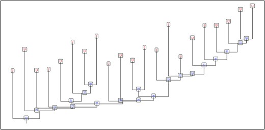
Dendrogram of the hierarchical structures extracted from H13CO+ (1–0) emission in G34. There are 41 structures including 21 leaves (labelled in red) and 20 branches (labelled in blue).
