


ABSTRACT
We investigate the joint density–velocity evolution in f(R) gravity using smooth, compensated spherical top-hats as a proxy for the non-linear regime. Using the Hu-Sawicki model as a working example, we solve the coupled continuity, Euler, and Einstein equations using an iterative hybrid Lagrangian–Eulerian scheme. The novel aspect of this scheme is that the metric potentials are solved for analytically in the Eulerian frame. The evolution is assumed to follow GR at very early epochs and switches to f(R) at a pre-determined epoch. Choosing the ‘switching epoch’ too early is computationally expensive because of high frequency oscillations; choosing it too late potentially destroys consistency with ΛCDM. To make an informed choice, we perform an eigenvalue analysis of the background model which gives a ballpark estimate of the magnitude of oscillations. There are two length scales in the problem: the comoving Compton wavelength of the associated scalar field and the width of the top-hat. The evolution is determined by their ratio. When the ratio is large, the evolution is scale-independent and the density–velocity divergence relation (DVDR) is unique. When the ratio is small, the evolution is very close to GR, except for the formation of a spike near the top-hat edge, a feature which has been noted in earlier literature. We are able to qualitatively explain this feature in terms of the analytic solution for the metric potentials, in the absence of the chameleon mechanism. In the intermediate regime, the evolution is profile-dependent and no unique DVDR exists.
1 INTRODUCTION
Observations of type IA supernovae have established that our Universe is undergoing a phase of accelerated expansion. The best explanation so far, is that this acceleration is due to an additional constant energy density component – called the cosmological constant (Λ). On galactic scales, observations of galaxy rotation curves have established the need for a non-baryonic matter component. In the standard ΛCDM model, our Universe today is made up of about 68 per cent of Λ, 28 per cent of dark matter, and 4 per cent baryonic or visible matter (Planck Collaboration VI 2020). While this model agrees remarkably well with a host of other observational constraints, there are still some glaring issues. The physical origin of Λ and dark matter are still unknown. On the observational side, recent measurements indicate that CMB estimates of the Hubble constant (H0) and the amplitude of fluctuations (σ8) are in disagreement with other probes of the same quantities (for e.g. Macaulay, Wehus & Eriksen 2013; Di Valentino et al. 2021). Thus, the need arises to explore models beyond ΛCDM. There are two broad avenues that have been considered. One path continues to assume that the observed acceleration is due to an additional ‘dark energy’ component and a plethora of phenomenological models have been explored. The other path assumes that there is no additional energy density, but instead postulates that Einstein’s General Relativity (GR) is incorrect and needs modification (see reviews by De Felice & Tsujikawa 2010; Sotiriou & Faraoni 2010; Clifton et al. 2012; Joyce et al. 2015; Joyce, Lombriser & Schmidt 2016; Nojiri, Odintsov & Oikonomou 2017 for various aspects of this subject). Current and future cosmological surveys aim to constrain modified gravity (MG hereafter) models through a host of observables. The number counts of clusters, their density and velocity profiles, the splashback radius and weak lensing maps are some of the important cluster-scale probes that will help constrain model parameters. Similarly, redshift-space distortions that give estimates of galaxy peculiar velocities also provide complementary constraints (see the recent review by Baker et al. 2021).
All of the above-mentioned investigations of the density–velocity divergence relation (DVDR), also sometimes called the velocity–gravity relation have assumed standard GR. One of the important features of standard GR is that the ‘Newtonian’ gravitational potential Ψ, which dictates particle dynamics and appears in the Euler equation is the same as the potential Φ that governs the spatial curvature and is related to the density through the Poisson equation. This equality is violated in most MG models and an extra equation is necessary to evolve the two potentials simultaneously. This changes the fundamental structure of the evolution equations and the interplay between the continuity and Euler equations which couples the density and velocity is different for MG as compared to GR (see figs 1 of Uzan 2007 and Song & Doré 2009 for nice schematics).
In this paper, we aim to understand the joint density–velocity dynamics using the spherical collapse model as a proxy for the non-linear regime. In the linear regime, the DVDR arises from imposing the ‘slaving condition’. It implies that the velocity field is proportional to the acceleration field and is such that there are no perturbations at the big bang epoch. In first order Eulerian perturbation theory, this is equivalent to ignoring the decaying mode in the linear solution for δ (Peebles 1980) and in Lagrangian perturbation theory, it is embedded in the Zeldovich approximation (Zel’Dovich 1970; Buchert 1992). In Nadkarni-Ghosh (2013), it was shown that it is possible to extend this same idea to the non-linear regime to obtain the non-linear DVDR. In a spherically symmetric system, the condition of no perturbations at the big bang, sets a specific relation between the non-linear δ and Θ at any epoch. This relation traces out a special curve in the 2D δ − Θ phase space, which was termed as the ‘Zeldovich curve’ and it was shown that this curve is an invariant set of the dynamical system given by the joint continuity and Euler equations, restricted to spherical symmetry. This means that the curve depends only on the cosmological parameters that govern evolution and not on initial conditions. Perturbations starting anywhere in phase space asymptote to the Zeldovich curve as they evolve. Nadkarni-Ghosh (2013) also showed that this invariance can be potentially exploited to break parameter degeneracy between parameters that govern initial conditions such as σ8 or ns and those that govern evolution such as Ωm or the equation of state w. In this paper, we evolve smoothed, compensated spherical top-hat overdensities and examine the resulting density and velocity profiles using a similar phase space description. Is there a unique relation between the density and velocity divergence akin to GR that is invariant of the initial conditions? For simplicity, we focus on the f(R) model and in particular consider the form given by Hu & Sawicki (2007).
Spherical collapse (SC) in the context of MG has been considered by various authors. Schäfer & Koyama (2008) used the Birkoff’s theorem to write equations of motions for the outer radius of a top-hat for a phenomenological model that interpolated between ΛCDM and the DGP model. They argued that although Birkoff’s theorem is known to be violated in most modified gravity models (Dai, Maor & Starkman 2008), the error associated with this approximation was small. Schmidt, Hu & Lima (2010) coupled SC with the halo model to compute the halo mass function, halo bias, and the non-linear matter power spectrum for the DGP theory. Chakrabarti & Banerjee (2016) investigated collapse in f(R) theories with a perfect fluid to understand the nature of the singularity. In standard GR, SC is most commonly used to compute the critical overdensity for collapse δc, an important ingredient of excursion set based approaches such as the Press–Schecter formalism and its extensions (Press & Schechter 1974; Sheth, Mo & Tormen 2001; Paranjape, Sheth & Desjacques 2013). The same is true in MG models. Herrera, Waga & Jorás (2017) computed δc for f(R), whereas Li and collaborators gave excursion estimates of the mass function in Galileon and chameleon models and also investigated the effect of the environment & Lam (Li & Efstathiou 2012; Li & Lam 2012; Barreira et al. 2013). Martino, Stabenau & Sheth (2009) computed cluster counts in MG for a Yukawa-like potential. Very recently, SC has also been combined with Large Deviations Theory to make analytic predictions of the matter density probability distribution function (Cataneo et al. 2021). Many of the above investigations model SC in modified gravity similar to that in standard GR, but with a modified effective Newton’s constant.
The treatment of spherical collapse in this paper is akin to that of Borisov, Jain & Zhang (2012) and Kopp et al. (2013) who solve the coupled continuity, Euler, Poisson, and scalar field equations iteratively for an f(R) model. Borisov et al. (2012) solve it in the Lagrangian frame by computing the acceleration of spherical shells at each step, whereas, Kopp et al. (2013) solve the system directly in the Eulerian frame as a coupled non-linear PDE using realistic profiles obtained from peaks theory (Bardeen et al. 1986). However, our treatment differs from these papers in some important aspects. First, we assume that the Compton wavelength is purely time-dependent and does not depend on the density of the perturbation. With this approximation, we cannot model the chameleon screening mechanism wherein the Compton wavelength changes with the density of the perturbation (Khoury & Weltman 2004). However, we illustrate the effect of screening by considering different scales for the width of the top-hat and demonstrate the scale-dependent nature of non-linear evolution. Secondly, we assume that the perturbations obey GR at early epochs and switch to the f(R) evolution at a relatively late time denoted as aswitch. This is necessary because the f(R) model exhibits high frequency oscillations at early epochs (Hu & Sawicki 2007; Song, Hu & Sawicki 2007) making the equations numerically stiff and computationally expensive. However, starting the evolution too late, destroys consistency with the background ΛCDM evolution. Thus, the switching epoch, needs to be chosen judiciously. In this paper, we perform an eigenvalue analysis of the background equations to estimate the magnitude of oscillations and make an informed choice of aswitch. Such an analysis has not been presented in the literature thus far. Finally, we do not solve the equations for the scalar field, but instead, recast the new degree of freedom in terms of the variable χ which is proportional to the difference of the two perturbation potentials Φ and Ψ. We present a closed form analytic solution for χ in spherical symmetry. We solve the system using a hybrid Lagrangian–Eulerian iterative scheme, wherein, the spatial equations for the two potentials are solved analytically in the Eulerian frame and the continuity and Euler equation are solved in the Lagrangian frame by recasting them as second-order evolution equations for the radii of a series of concentric shells.
The rest of the paper is organized as follows. In Section 2 we define the Hu-Sawicki system and perform the eigenvalue analysis of the same. Section 3 lays down the set of equations and initial conditions governing the non-linear evolution. Section 4 outlines the iterative method of solution and gives analytic expressions for the potential χ. In order to illustrate screening, we plot the static solutions to the potentials as a function of the radial coordinate for different choices of the perturbation scale. Section 5 evolves the compensated top-hat profile in the linear regime and Section 6 extends the evolution to the non-linear regime. The late time density and velocity fields are analysed by plotting them on the density–velocity divergence phase space and fitting formulae are provided in certain limits. We summarize in Section 7. The appendix Section A gives the details of the initial top-hat setup and Section B gives the details of the error tests performed to validate the numerical code.
2 BACKGROUND COSMOLOGY IN THE HU-SAWICKI MODEL
2.1 Equations of motion
2.2 Consistency with ΛCDM
Consistency with ΛCDM demands that weff be close to −1. We find that weff is oscillatory and in particular the deviation from the ΛCDM value depends sensitively on the starting epoch ainit. Fig. 1 shows weff for two values of fR0 and three values of ainit: 0.2, 0.1, and 0.05 corresponding to z = 4 (blue), 9 (red), and 19 (black), respectively. In order to compare with Hu & Sawicki (2007), we choose Ωm, 0 = 0.24 and ΩΛ, 0 = 0.76 for this analysis but the discussion is not sensitive to this choice. From the left-hand panel, it is clear that the deviation from ΛCDM at lower redshifts is less when the system has a higher starting redshift. However, the oscillation frequency is higher at higher redshifts. Computationally, this means that the equations are more ‘stiff’ requiring a higher number of steps when starting at a higher redshift. This behaviour poses a challenge: starting evolution too early is computationally expensive whereas starting too late implies greater deviation from the ΛCDM equation of state. This challenge is somewhat mitigated when smaller values of |fR0| are considered (right-hand panel). The equations remain computationally stiff at high redshifts, however, the oscillation amplitude is significantly reduced implying an evolution very close to ΛCDM. For ainit = 0.2, the deviation of the equation of state, from its ΛCDM value, in the dark energy dominated era can be more than 5 per cent when fR0 = −0.01 and is less than 0.05 per cent when fR0 = −10−6. Thus, for parameter values of this model that satisfy Solar system constraints, the oscillatory behaviour can be circumvented by starting the evolution later. In order to understand this behaviour better and make an informed choice about the starting redshift, we examine the above system by analysing the eigenvalues which give insights into the nature of oscillations.
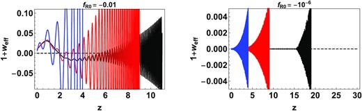
The deviation of the effective equation of state from its ΛCDM value as defined in equation (16) for fR0 = −0.01 (left-hand panel) and fR0 = −10−6 (right-hand panel) plotted for three different starting epochs: zinit = 4 (blue), 9 (red), and 19 (black). The solutions are oscillatory. The amplitude of deviation is high at earlier epochs and decreases as the evolution proceeds. Thus, consistency with ΛCDM at low redshifts i.e. in the ‘dark energy era’ is better if the evolution is started earlier. However, the oscillation frequency is higher when the evolution is started earlier making the system numerically ‘stiff’. The right-hand panel shows that this deviation is significantly smaller for smaller values of |fR0|, however the oscillation frequency is higher (see Fig. 2).
2.3 Eigenvalue analysis of the Hu-Sawicki background cosmology
Fig. 2 shows the eigenvalues of |${\mathcal {A}}_{\rm lin}$|. The black solid line and red dashed lines correspond to fR0 = −0.01 and fR0 = −10−6, respectively. The eigenvalues are complex. The left-hand panel shows the real part of the eigenvalue, which is negative, indicating that the amplitude of the oscillations decreases as evolution proceeds. The right-hand panel shows the imaginary part which indicates the instantaneous frequency of oscillations. The figure shows two distinct regimes. At very high redshifts, the oscillation frequency is large and decreases as a power law in a: |$|\rm {Im}[\nu ]| \sim a^\alpha$|. The best-fitting value was found to be α ∼ −3. At low redshifts, the instantaneous frequency is almost a constant. The epoch where these two asymptotes cross is marked as the transition epoch atrans ∼ 0.34 corresponding to a redshift of around z ∼ 2. For a smaller value of |fR0|, the magnitude of the imaginary part is higher implying higher frequency oscillations at the same redshift. However, we find that the transition epoch is independent of |fR0| and also independent of the value of Ωm, 0 for flat models. For ainit < <atrans, the high frequency oscillations make the system ‘numerically stiff’ and evolving the system is computationally expensive.
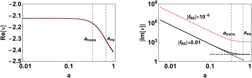
Instantaneous eigenvalues of the linearized matrix |${\mathcal {A}}$| given by equation (18). The red dashed line indicates fR0 = −10−6 and the black solid line indicates fR0 = −0.01; both models have n = 1. The eigenvalues are complex implying oscillations. The real part (left-hand panel) is negative implying that the oscillation amplitude decreases as a increases. The imaginary part, which determines the oscillation frequency is large at early epochs and decreases as a power law in a and levels off as a approaches 1. atrans denotes the epoch where the two asymptotes cross. At the same redshift, the instantaneous oscillation frequency is larger for smaller values of |fR0| but the transition value is independent of fR0. The initial amplitude is lower for smaller values of |fR0| (not shown here), but the rate of decrease is independent of |fR0| as indicated by the real part.
The perturbed system described in the next section also exhibits oscillations akin to the background. In this paper, we have expressed the perturbation equations in terms of two temporal evolution equations for the density and velocity and two spatial equations for the metric potentials. This form of the equations is not amenable to the eigenvalue analysis discussed above. However, in order to overcome the issue of numerical stiffness we adopt the following strategy. We evolve the perturbations in standard GR starting from an early epoch ainit = 0.001 to a late epoch aswitch, after which the evolution ‘switches’ over to f(R) gravity. Following the insight gained from the eigenanalysis of the background we choose aswitch to be in the vicinity of atrans. In particular, we choose aswitch = 0.1. It is possible to choose aswitch in a more quantitative manner by setting tolerances for deviation of equation of state or numerical stiffness, but we do not follow such a strategy here. We are interested in the qualitative differences in non-linear growth between the GR and f(R) models. Furthermore, the DVDR, if such a unique relation exists, should depend only on the evolution equations and not on the choice of aswitch. Thus, it suffices to consider only a single choice for aswitch and we do not investigate the dependence of non-linear growth on this parameter. Clearly, choosing aswitch earlier (later) will increase (decrease) the effect of the modification.
High frequency oscillations in the Hu-Sawicki model have been referred to in the original paper (Hu & Sawicki 2007) as well as in follow up studies (Elizalde et al. 2012). They have also been encountered in the context of evolution of designer models (Song et al. 2007) as well as in linear perturbations (see e.g. Pogosian & Silvestri 2008; Lima & Liddle 2013; Silvestri, Pogosian & Buniy 2013). The issue of ΛCDM consistency has been explicitly addressed in the literature (e.g. Appleby & Battye 2007; Starobinsky 2007; Ceron-Hurtado, He & Li 2016; Chakraborty, MacDevette & Dunsby 2021). Some of these studies have been in the context of finding stable f(R) models. We note that stability in the Hu-Sawicki model is guaranteed by the choice of parameters. The system is oscillatory but stable since the amplitude of oscillations decays as evolution proceeds. To the best of our knowledge, an understanding of the oscillatory behaviour based eigenvalue analysis of this system has not been presented so far in the literature.
2.4 Compton wavelength
Fig. 3 shows the relevant scales and epochs on a plot in the k − a plane. aeq corresponds to the epoch when the dark energy density is equal to the matter density in the background evolution. atrans denotes the epoch when frequency of oscillations in the Hu-Sawicki background starts to level off. Starting evolution for a < <atrans is computationally expensive where as a > >atrans implies significant deviations from the ΛCDM background, particularly for larger values of |fR0|. atrans provides a estimate of the optimal epoch to start evolution. At early epochs, the cosmologically relevant scales (∼1h−1Mpc) are well above the Compton wavelength and one cannot expect to see departures from GR on those scales. Coincidentally, for fR0 values which are allowed by Solar system and galactic constraints the Compton wavelength becomes greater than ∼1h−1Mpc at around a ∼ atrans.
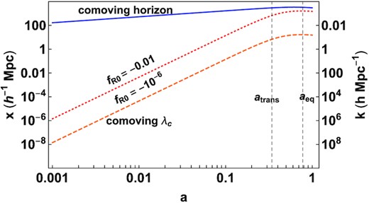
Important scales in the model marked on a k − a plane (left-hand panel). The red dotted and orange dashed lines denote the comoving Compton wavelength xC of the scalaron field implied by the Hu-Sawicki model for fR0 = −0.01 and fR0 = −10−6, respectively. At any epoch, the effects of modified gravity begin to manifest when x ≲ xC. The blue solid line indicates the scale when the given mode crosses the horizon. aeq denotes the epoch of dark energy–matter equality and atrans is the epoch when the frequency of oscillations in the Hu-Sawicki background start to level off to a constant.
3 EQUATIONS FOR NON-LINEAR PERTURBATIONS
3.1 Equations
In this work, we assume that |${\bar{x}_C}$| depends only on the value of fRR in the background and does not change with the perturbation. As a result, we do not capture the ‘chameleon screening mechanism’ wherein the Compton wavelength is small in high density regions; this is responsible for satisfying Solar system constraints (Khoury & Weltman 2004; Hu & Sawicki 2007). Nevertheless, we are able to illustrate ‘screening’ by considering perturbations of differing length scales xtop for a fixed fR0. We consider three values of xtop = 0.002, 2, and 200 h−1Mpc, which for fR0 = −10−6 gives Q = 1217, 1.21, 0.012 at a = 1, respectively. We refer to Q > >1 and Q < <1 as the ‘strong’ and ‘weak’ field regimes, respectively. The evolution of Q for these three scales is shown in Fig. 4. Note that, for xtop ∼ 0.002h−1Mpc, Q > 1 and for xtop ∼ 200h−1Mpc, Q < 1 from a = 0.1 to today and they can be considered as being ‘strong’ and ‘weak’ perturbations over the entire domain of evolution. In what follows, we will refer to the three perturbations with their value of Q today and ignore the temporal evolution of Q.
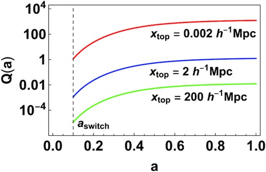
The parameter |$Q = {\bar{x}}_{C}/(x_{\rm top})$| plotted as a function of a for the three values of top-hat widths considered in this paper. The dotted line denotes aswitch, which is the epoch at which evolution is assumed to switch from GR to f(R). In the text, we characterize these three fluctuations by their value of Q today and ignore the time dependence.
4 METHOD OF SOLUTION
4.1 Outline
4.2 Lagrangian coordinates
4.3 Equations in the hybrid Eulerian–Lagrangian scheme
4.4 Initial conditions
4.5 Algorithm
Notation: Let ainit and afinal denote the initial and final epochs of interest and aswitch denote the epoch where the evolution switches from GR to f(R). The time between aswitch, to afinal is divided into Nt intervals equi-spaced in ln a. Let a0 = ainit, a1 = aswitch, |$a_{N_t} = a_{\rm final}$| and a2, a3… denote intermediate epochs. At any epoch an, the data at the start of the time interval is defined on a 1-d grid with Ns points uniformly spaced in ln x space. These correspond to radial shells. xi(an), i = 1, 2, …Ns denotes the Eulerian position of the i-th shell at the start of the n-th step. At an, the Lagrangian coordinate of the shell i-th shell is defined as qn, i = xi(an). The density and velocity are known at the time an on the uniform grid and are given by δi(qn, an) and vi(qn, an). Here we drop the subscript ‘i’ on qn but it is understood that qn is different for each ‘i’.
At the end of the step, i.e. at an + 1, the Eulerian position, density, and velocity of the i-th shell are denoted as xi(qn, an + 1), δi(qn, an + 1) and vi(qn, an + 1). However, the Eulerian positions xi(qn, an + 1), i = 1, 2, …Ns are not equi-spaced. At an + 1, a new grid is defined in Eulerian space which is equi-spaced in ln x over the range xmin to xmax, where xmin and xmax correspond to the Eulerian location of the innermost and outermost shell at an + 1. This uniform grid is denoted as |$x_{i^{\prime }}(a_{n+1}), i^{\prime } = 1, 2 \dots N_s$|. The i′ indicates that the shell locations are re-defined after each step. Thus, |$x_i(q_n, a_{n+1}) \ne x_{i^{\prime }}(a_{n+1})$|. The number of shells are the same at each step since no shells have collapsed or crossed. The Lagrangian coordinate at an + 1 is given as |$q_{n+1,i^{\prime }} = x_{i^{\prime }}(a_{n+1})$|. The density and peculiar velocity are obtained by interpolating δi(qn, an + 1) and vi(qn, an + 1) on to the uniform grid. They are denoted as |$\delta _{i^{\prime }}(q_{n+1}, a_{n+1})$| and |$v_{i^{\prime }}(q_{n+1}, a_{n+1})$|, respectively. Step 1. GR evolution:
Evolve the system from a0 = ainit to a1 = aswitch using equation (50) and initial conditions equation (52).
Construct the Eulerian position, density, and velocity at a1 using equations (41) and (42). This gives xi(q0, a1), δi(q0, a1), and vi(q0, a1) for each shell i, i = 1…Ns.
Re-initialize the system by defining a uniform grid in ln x space, define the new Lagrangian coordinate q1, and interpolate the density and peculiar velocity to get |$\delta _{i^{\prime }}(q_1, a_1)$| and |$v_{i^{\prime }}(q_1, a_1)$|.
Step 2. f(R) evolution:
At a1, and at any an thereafter, first solve the spatial equations, equations (46) and (47), setting a = an and x = qn. The solutions for Φ+ and χ can be obtained analytically and are given in the next section. These expressions are evaluated numerically using the values of δi(qn, an) known at the start of the step a = an.
Using the solutions for Φ+ and χ compute the r.h.s of equation (45) i.e. ∇qΨ(q, a) = ∇qΨ(q, an) at each shell i. We assume that throughout the interval an to an + 1, ∇qΨi(qn, a) = ∇qΨi(qn, an) i.e. the force is constant.
- Compute the temporal evolution between an and an + 1 using equation (45). There are Ns such equations, one for each shell. Let Ai denote the scale factor of the i-th shell. The initial conditions are(53)$$\begin{eqnarray*} A_i(q_n,a_n) = 1 \,\,\,\,\,\, {\rm and} \,\,\,\,\,\,A_i^{\prime }(q_n,a_n) = \frac{v(q_n, a_n)}{a_nH(a_n) q_n} \end{eqnarray*}$$
Construct the density and velocity at an + 1 using equations (41) and (42). This gives xi(qn, an + 1) and δi(qn, an + 1) and vi(qn, an + 1) for the i-th shell. Compute the end-points xmin and xmax at an + 1 to be the Eulerian positions of the innermost and outermost shells.
Re-initialize: define a new uniform grid over the range xmin and xmax denoted by |$x_{i^{\prime }}(a_{n+1}), i = 1, 2 \dots N_s$|. Define the new Lagrangian coordinate |$q_{n+1} = x_{i^{\prime }}(a_{n+1})$| and interpolate the data given by δi(qn, an + 1) and vi(qn, an + 1) on to this uniform grid to get the initial data for the next step |$\delta _{i^{\prime }}(q_{n+1}, a_{n+1})$| and |$v_{i^{\prime }}(q_{n+1}, a_{n+1})$| at equi-spaced shell positions.
Go to step 2(i) until an + 1 = afinal.
4.6 Analytic solutions for the potentials
Fig. 5 shows the solution for the dimension-less χ (second panel), ∇χ (third panel), and the potentials Φ and Ψ (fourth panel) as a function of x for the density profile δ corresponding to a smooth compensated top-hat (top-panel). The solution for χ is evaluated at a = 1 for fR0 = −10−6. The |${\bar{x}}_C$| for this fR0 at a = 1 is 2.43 h−1Mpc. To illustrate how χ changes with the choice of scale we pick three values for the width of the top-hat denoted by xtop = 0.002, 2, and 200 h−1Mpc. This corresponds to Q = 1217, 1.21, 0.012, respectively. Changing the choice of scale is also equivalent to changing the value of fR0. The effect of the fifth force depends on ∇χ. It is clear from the third panel, that when Q < <1, the extra force ∇χ is non-zero only at the edge of the top-hat. In such a system, the evolved density develops a ‘spike’ at the top-hat boundary (see Section 6.4). This phenomenon has been reported in the literature before (Borisov et al. 2012; Kopp et al. 2013; Lombriser 2016), but in the context of the chameleon mechanism. Here, we provide a mathematical explanation of this feature based on the analytic solution, but in the absence of chameleon screening. A more detailed discussion can be found in Section 6.4. The lowest panel shows the two potentials Φ and Ψ. When Q > >1, the two potentials clearly differ, when Q < <1, the effect of the ‘extra force’ is effectively ‘screened’ and the two potentials almost coincide as is expected in standard GR. The difference in the two potentials is related to χ, which is suppressed by a factor of Q2 in this regime.
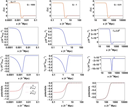
The spatial solutions for dimension-less χ, ∇χ, Φ and Ψ at a = 1 corresponding to a smoothed top-hat source δ(x) (top-panel). In the strong field limit Q > >1, the effect of the modification is the strongest corresponding to the largest difference between Φ and Ψ. In the weak field limit, Q < <1, the solution for χ is proportional to δ and the ‘extra force’ which is proportional to ∇χ is largest at the edge of the top-hat. The amplitude of this additional force is small compared to the potentials and they are effectively equal as is expected in standard GR.
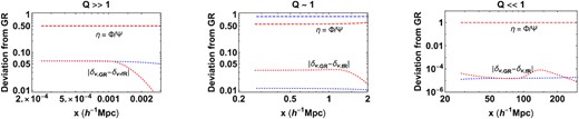
Equation (46) implies that the potential Φ+ has the same equation as the Newtonian potential in standard GR. We denote Φ+ = ΨGR. In the strong field limit, χ ≈ −2/3Φ+ which gives Ψ ≈ 4/3ΨGR, whereas in the weak field limit Ψ ≈ ΨGR. Fig. 6 shows the ratio Ψ/ΨGR, evaluated at the innermost shell, as a function of the parameter Q of the profile. The strong and weak field asymptotic values are clearly in agreement with expectations. Since, the three values of Q above were not sufficient to characterize this plot, the static potentials were evaluated for additional profiles with different values of Q. The details can be found in Appendix A.
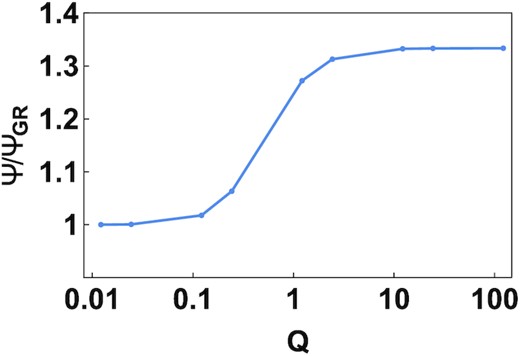
The ratio Ψ/ΨGR evaluated at the innermost shell for profiles with different values of Q. In f(R), the ‘Newtonian potential’ Ψ i.e. the potential Ψ, that appears in Euler’s equation is enhanced. In the strong field limit, Q > >1, the ratio Ψ/ΨGR ∼ 4/3. In the weak field limit, Q < <1, the ratio asymptotes to unity.
5 LINEAR EVOLUTION
To confirm the expectations in the linear regime, we evolve a compensated top-hat density from ainit = 0.1 up to two final epochs afinal = 0.2 and afinal = 0.4 and for two values of Q: Q ∼ 1217 and Q ∼ 1.21. The Q < <1 is not expected to show significant deviation from GR. Since the evolution is over a small time interval, it suffices to use a small number of steps: Nt = 40. The initial velocity is set by assuming Zeldovich initial conditions. The initial and final densities are plotted in Fig. 7. The dashed orange corresponds to the initial profile and the black line is the theoretically expected, linearly evolved profile in GR, the red-dotted line is the numerically evolved profile using the non-linear code for the Hu-Sawicki model with fR0 = −10−6 and the cyan line is its theoretical expectation given by multiplying the profile with the scaled linear growth factor defined in equation (63). For the Q > >1, the cyan and the red-dotted lines coincide at both a = 0.2 and a = 0.4. Their deviation from the corresponding GR value is larger for larger final epochs. This serves as a code check of the non-linear code in the linear regime. For Q ∼ 1, the red-dotted lines and the cyan lines do not coincide because equation (62) is no longer valid. The red-dotted lines are now closer to the GR values because the strength of the modification reduces as Q decreases. It is important to note that the linear growth given by equation (62) is in real space. In Fourier space, it is possible to write a linear growth equation for each mode δk which is valid for all scales, but is scale-dependent (see for e.g. Bean et al. 2007; Pogosian & Silvestri 2008). Most current and upcoming large-scale structure surveys aim to constrain modified gravity parameter by measuring the linear growth rate of perturbations. Most of these analyses are scale-independent i.e. they only look for a deviation from the growth rate in GR (for e.g. Alam et al. 2021). Although, a systematic scale-dependent measurement of the growth rate is ideal, scale-independent measurements can be used to place upper limits on the Compton wavelength of the scalaron field.
Evolution in the linear regime. The left-hand panel shows the initial density profile (orange, dashed), the expected final density in GR (black, solid), the theoretically expected (cyan), and the numerically (red, dotted) evolved final density in the f(R) model at two final epochs. The cyan and red dotted curves coincide implying the correct linear evolution for Q > >1 given by the scale-independent equation (62). The right-hand panel shows the same data for a profile with Q ∼ 1. The cyan and red-dotted curves deviate since the scale-independent linear growth equation is no longer valid. The deviation from GR is higher in the strong field regime (Q > >1) as compared to the intermediate field regime (Q ∼ 1) as expected.
6 NON-LINEAR REGIME
6.1 Non-linear density and velocity
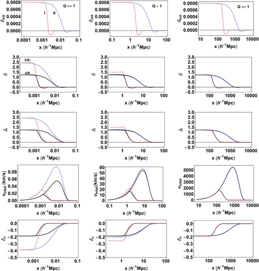
Initial δ at a = 0.001 and the non-linearly evolved δ, Δ, infall velocity and relative Hubble velocity (δv) at a = 1 for three values of the top-hat scale |$x_{\rm top} = 0.002, 2, 200\, h^{-1}{\rm Mpc}$| corresponding to Q > >1, Q ∼ 1, and Q < <1, respectively. The red and blue dotted curves correspond to σ = 0.0025 (profile I) and σ = 0.1 (profile II) evolved with the Hu-Sawicki model with fR0 = −10−6. The solid curves denote the evolution using standard GR from a = 0.001 to a = 1 for the same. The evolution in GR is scale independent. Thus, the final profiles are the same for all values of Q. For the f(R) model, when Q > >1, the evolution equations are structurally similar to GR with an enhanced potential. So the evolved profiles I and II coincide in the interior similar to the GR case, but with an increased final density. When Q < <1, the scale is outside the Compton scale making the system seemingly indistinguishable from GR. When Q ∼ 1, the evolution is scale-dependent and hence profile dependent.
In the ΛCDM model, the radial evolution of a shell depends only on the initial average density at the shell location and is independent of the size of the shell (see equation 50). Consequently, in the GR case, the final density profiles for the two σ values, coincide in the interior of the top-hat since the initial density in the interior is same for both profiles. Because of the scale-independent evolution, the final density profiles in GR are the same for all values of Q. The magnitude of the velocity depends on the scale but the dimension-less quantity δv defined in equation (65) is also independent of Q.
In the f(R) model, the evolution is, in general, scale-dependent. The evolution of the extra potential χ depends sensitively on the parameter Q. In the strong field regime when Q > >1, the structure of the equations is similar to that of GR. The final densities in the interior of the top-hat are independent of σ as is the case in GR, but because the potential is enhanced by a factor of 4/3, the final density of the top-hat is higher as compared to GR. In the intermediate regime, when Q ∼ 1, the evolution is profile dependent. An un-smooth top-hat is described uniquely by a single scale xtop; smoothing broadens the top-hat edge increasing the effective width of the top-hat and decreasing the effective Q. Thus, the profile I (smaller σ) shows a greater density enhancement than profile II (larger σ). In the weak field regime, when Q < <1, the extra force is suppressed and the evolution is close to GR. There is expected to be some density enhancement at the edge of the top-hat as was discussed in Section 4.6 but it is too small to be seen on the scale of the plot. This effect is demonstrated in Section 6.
6.2 Phase space evolution
Finding such invariants of the dynamical system can be potentially useful in breaking parameter degeneracies as was illustrated in N13. This is because invariant sets depend only on cosmological parameters that appear as coefficients in the dynamical equations and are insensitive to the parameters that describe initial conditions, such as, the amplitude σ8 or spectral index ns. One of the primary aims of this paper is to understand if such invariants exist for the f(R) system. Because of the complexity of the equations, it is not practically feasible to implement the algorithm used in N13 to select the δ − Θ pairs that satisfy the ‘slaving condition’. Instead, we evolve the compensated top-hat profiles which start with Zeldovich initial conditions, compute the resulting density–velocity divergence pairs along the evolved curves and examine where they lie in phase space. Is the resulting curve in phase space universal? Or does it depend on the details of the initial profile?
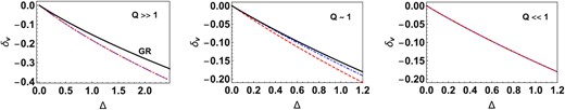
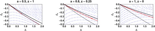
The spherically averaged density Δ and fractional Hubble parameter δv plotted on the Δ − δv phase space for profiles I (red, dotted) and II (blue, dot-dashed). In standard GR, the ‘slaving condition’ imposes a specific relation between the non-linear density and velocity which traces out a special curve in the phase space. This curve is an invariant of the dynamical system described by equations (69) and (70). In the f(R) model, in the strong field regime (Q > >1), the evolution is scale-independent and the dynamics can be described by equations (73) and (74) akin to standard GR and the non-linear relation between Δ and δv is profile independent. In the weak field limit (Q < <1), the curves coincide with the GR (ΛCDM) case. However, in the intermediate regime (Q ∼ 1), the Newtonian force is scale dependent and in the Δ − δv plane, the dynamics is profile dependent.
Deviation of the DVDR relation in modified gravity from that in GR at a = 1 corresponding to the curves in Fig. 9. The response of the velocity field to the matter is different in GR and modified gravity. The difference is directly correlated to the difference between the two potentials Ψ (which governs dynamics) and Φ (which governs the curvature). It is interesting to note that while Φ and Ψ vary along the radial direction (see Fig. 5), their ratio is a constant and directly correlated with deviation of the DVDR curve from its GR counterpart in phase space.
6.3 Fitting form for the DVDR in the strong field regime
Fig. 11 shows the fitting form for the DVDR relation for the ΛCDM case (black) and the f(R) model (red) in the strong field regime as a function of redshift. The red points represent the numerically evolved (Δ, δv) points corresponding to the selected epoch. The blue arrows show the streamlines of the flow given by equations (73) and (74). They show the instantaneous direction of the vector defined by |$(\Delta ^{\prime }, \delta _v^{\prime })$|. The system defined by equations (73) and (74) is a non-autonomous system since the coefficients of Δ and δv in the r.h.s. are time-dependent. Hence, the streamlines are not constant at all epochs and neither is the DVDR curve. This can be contrasted with the case of a pure Ωm = 1 flat universe, where the dynamical system for Δ − δv is an autonomous system and the DVDR relation is time-independent (see N13 for a detailed discussion).
The DVDR in the strong field limit (Q > >1). The red line is the fitting form given in equation (78) and the red dots show the Δ − δv pairs computed from the radial profile at the selected epoch. The solid black line shows the DVDR for the reference ΛCDM model considered here and the black dotted line shows the DVDR for the flat EdS model with Ωm = 1. The dynamical system of equations governing Δ and δv is non-autonomous in the case of ΛCDM and f(R) and hence the curves are time-dependent. On the other hand, the EdS curve is the same for all epochs.
The DVDR relation based on spherical collapse is one-to-one. However, for realistic density and velocity fields, there is a scatter around a mean relation. Numerical simulations in the case of ΛCDM have shown that the mean relation is close to that given by the spherical collapse model (Bernardeau et al. 1999; Kudlicki et al. 2000; Bilicki & Chodorowski 2008). This scatter is usually attributed to the non-local nature of gravity. The scatter can be related to the shear component of the velocity field as was shown by Chodorowski (1997) using perturbation theory and using triaxial collapse by Nadkarni-Ghosh & Singhal (2016). It remains to be checked whether the mean relation from the joint density–velocity PDF obtained from simulations agrees with the estimate based on spherical collapse given in this paper.
6.4 Density enhancement in non-linear evolution
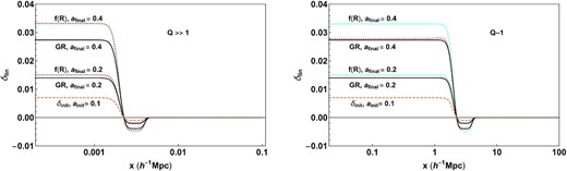
In this paper, we do not undertake a systematic study of the highly non-linear regime, in particular the process of collapse. However, we illustrate, qualitatively, the difference between highly non-linear evolution in the strong and weak limits. We consider two profiles: both with σ = 0.0025, but with different xtop. One case corresponds to xtop = 0.002h−1Mpc and the other with xtop = 200h−1Mpc. Q > >1 for the former and Q < <1 for the latter over the entire range of evolution from a = 0.1 to a = 1. In each case, the initial amplitude was chosen so that the final evolved density in the f(R) model has δ ∼ 100. This implies that in the strong field limit, the initial amplitude of the perturbation is less than that for the weak field limit. The details are in Appendix A. The resulting non-linear Δ is shown in the top-panel of Fig. 12 and the difference between the f(R) and GR profiles is shown in the bottom panel. For Q > >1, the amplification is large since the effective force is 4/3 times stronger. For Q < <1, the evolved profiles for f(R) and GR apparently coincide. However, the lower panel shows that the f(R) model has a higher density at the edge of the top-hat. This can be explained in terms of the solution for χ as was discussed in Section 4.6. χ is proportional to δ in this regime and the force which is proportional to the gradient is non-zero only at the edge of the top-hat.
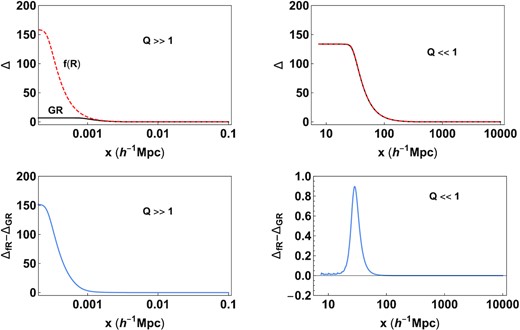
Demonstration of non-linear growth in strong versus weak regimes. In the upper panel, the red dashed denotes f(R) and black solid is the GR value for Δ at a = 1. In the strong regime Q > >1, the profile is amplified as compared to GR, whereas for the weak field regime, where Q < <1, the two profiles coincide by eye. The lower panel profile develops a cusp at the edge of the top-hat. This is related to the solution for χ which is proportional to the density in the weak field limit. Since the force is proportional to the ∇χ, this manifests itself as a cusp at the edge of the top-hat.
In the f(R) model, the scalar field corresponds to χ = δfR. The Q < <1 solution corresponds to |$\nabla _x^2 \chi \approx 0$|, which gives |$\chi = {\bar{x}}_c^2 H^2 \Omega _m a^2 \delta$|. Since the ‘fifth force’ depends on ∇xχ, it is zero everywhere except at the edge of the top-hat, where the derivative of the density is non-zero. However, we do not refer to this as ‘chameleon screening’ since the Compton wavelength is constant both inside and outside the top-hat and is independent of δ. This can also be seen by defining an ‘effective potential’ |$V_{\rm eff}(\chi) = \frac{\chi ^2}{2{\bar{x}}_C^2} + H^2 \Omega _m a^2 \delta \chi$|, recasting the equation for χ as |$\nabla _x^2 \chi = V_{\rm eff}(\chi)_{,\chi }$| and noting that the second derivative, Veff, χχ, which is inversely related to the Compton wavelength, is independent of δ. In this paper, we have used the first order of the Taylor expansion |$\delta f_R \sim f_{RR} \delta R + \mathcal {O}(R)$| in obtaining a linear equation for χ. Ideally, as has been argued by Hu-Sawicki, this linearization is not valid when δR is large (high curvature limit). Alternately, it is clear that when the Compton wavelength is small i.e. fRR is small, higher order corrections to this expansion may become important making the equation for χ non-linear. Higher order terms can be modelled by allowing the Compton wavelength to depend on χ. Thus, the chameleon solution is essentially a solution of the non-linear equation for χ.
7 SUMMARY AND DISCUSSION
In this work, we have investigated the non-linear evolution of cosmological perturbations in f(R) models using the compensated spherical top-hat as a proxy for the non-linear regime. Our algorithm is an iterative hybrid Lagrangian–Eulerian scheme; the continuity equation and Euler equation are solved in Lagrangian coordinates and the equations for the metric potentials are purely spatial and are solved analytically in Eulerian space. Specifically, we chose the Hu & Sawicki (2007) model for simplicity, with majority of the results obtained by setting fR0 = −10−6 and n = 1. The evolution equations depend upon the ratio of |$Q = {\bar{x}_C}/{x_{\rm top}}$|, where |${\bar{x}_C}$| is the reduced comoving Compton wavelength of the model given by equation (23). The Compton wavelength is assumed to depend only on the background cosmology; thus we do not model the chameleon screening mechanism (Khoury & Weltman 2004). However, we demonstrate the role played by the Compton wavelength by changing the scale of the top-hat (xtop). We consider three values of xtop = 0.002, 2, and 200 h−1Mpc, corresponding to Q = 1217, 1.21, and 0.012 at a = 1. There are several new features of this work.
Analysis of oscillations in the background evolution
It is well known that the f(R) model exhibits high frequency oscillations at high redshifts, both in the background and perturbation evolution making the system numerically stiff. To overcome this, it is favourable to assume GR at early epochs and ‘switch’ to f(R) evolution at a late epoch denoted by aswitch. By performing an eigenvalue analysis of the linearized background equations, we were able to assess the nature of oscillations and make an informed choice of aswitch. Such an eigenanalysis has been performed for the Boltzmann hierarchy in order to gain insights for optimizing solvers (Nadkarni-Ghosh & Refregier 2017) and a similar analysis can also be performed for the linear perturbation system of f(R) or other models of modified gravity. In particular, it could help us in putting the Quasi-Static-Approximation on firmer grounds (Hojjati et al. 2012; Sawicki & Bellini 2015; Pace et al. 2021).
Analytic solutions for the metric potentials and density-enhancement
Growth of perturbations in standard GR is governed by the joint continuity, Euler and Poisson equations. In f(R) models, there is an extra equation corresponding to the ‘extra’ degree of freedom, usually encapsulated by the variable fR. In the limit |fR| < <1 and |f/R| < <1, the perturbations in fR can be expressed as the difference of the two potentials Φ − Ψ, where Φ and Ψ are the metric perturbations corresponding to the ‘curvature’ potential and ‘Newtonian’ potential, respectively. We derive an analytic solution for χ = Φ − Ψ in real space in spherical symmetry valid for all values of Q. In the strong field limit, when the scale of the perturbation is much less than its Compton wavelength (Q > >1), χ obeys the Poisson equation and Ψ is 4/3 times its value in standard GR. In the weak field limit, when the scale of the perturbation is much greater than its Compton wavelength (Q < <1), χ ∝ δ. This means that the force, which is proportional to the gradient of χ is non-zero only at the edge of the top-hat. This results in a density enhancement at the top-hat edge, a phenomenon that has been previously reported in the literature (Borisov et al. 2012; Kopp et al. 2013) in the context of ‘chameleon screening’. Here we demonstrate the same effect in the absence of a chameleon mechanism. If the Compton wavelength is allowed to change within the perturbation, then the resulting equation for χ is non-linear, possibly enhancing this effect. A more quantitative exploration is left for future investigations. Nevertheless, the analytic solutions presented here can also serve as a ‘test case’ to check other numerical schemes, similar in spirit to the use of spherical collapse as a ‘control case’ for numerical simulations (see Joyce & Labini 2012).
Phase space analysis of evolution of perturbations and the density–velocity divergence DVDR relation in the strong field limit
We evolve the compensated top-hats and examine the evolution of the perturbations in the 2D density–velocity divergence phase space. For the radially varying profiles, it is easier to compute the Δ − δv pairs instead of the δ − Θ pairs, where Δ is the spherically averaged density and δv is the fractional Hubble velocity of the shell. In the strong field limit, where the evolution of perturbations is scale-invariant, it is possible to define a unique DVDR relation and we give a fitting form for the same. In the intermediate field limit, Q ∼ 1, the evolution of perturbations is profile dependent and an invariant relation between δ and Θ does not exist. In the weak field limit, the dynamics is approximately that of GR.
There are several caveats in this work. The spherical collapse is a simplistic model: the system does not take into account any effect of the environment or rotations and ignores mode–mode coupling. The first step forward is to consider triaxial collapse. Triaxial collapse, which is an important ingredient in mock catalogue generators like PINOCCHIO (Monaco 2016; Rizzo et al. 2017; Moretti et al. 2020; Song et al. 2021) has not been studied in great detail in the context of modified gravity, albeit, with the exception of some recent efforts (Burrage, Copeland & Stevenson 2015; Burrage et al. 2018; Ruan, Zhang & Hu 2020). To capture the effects of mode coupling in the analytic framework, it is necessary to consider perturbation theory, either in the Eulerian or Lagrangian frame and related schemes (see e.g. Aviles & Cervantes-Cota 2017; Baojiu 2018; Aviles, Cervantes-Cota & Mota 2019; Valogiannis, Bean & Aviles 2020; Aviles et al. 2021). The hybrid Eulerian–Lagrangian scheme outlined here does not rely on spherical geometry. Equations (31)–(34) are general and the hybrid scheme can also be incorporated with a multistep Lagrangian perturbation theory (Nadkarni-Ghosh & Chernoff 2011, 2013), which guarantees convergence in ΛCDM models up until shell-crossing. However, convergence and shell-crossing related issues in modified gravity scenarios remain to be investigated (see for example Rampf & Frisch 2017; Rampf & Hahn 2020 for a discussion of these matters in standard GR). A code, called SELCIE, based on Finite Element Methods to solve the chameleon equations of motion in arbitrary mass distributions has recently been developed by Briddon et al. (2021). However, it is currently not set up to perform temporal evolution of the matter distribution in the presence of chameleon screening. It may be possible to couple iterative methods used in this paper with such tools. In addition, for the f(R) model considered here, the relevant scales for which the system is in the strong field limit, are not cosmological scales, but correspond to smaller bodies governed by additional astrophysical processes which have also been ignored in this treatment.
The f(R) model, in the metric formalism can be considered as a special case of Brans–Dickie theories, which in turn belongs to the more general class of Horndeski theories (De Felice & Tsujikawa 2010; Kobayashi 2019). More recently, the effective field theory of dark energy has become a popular formalism which is aimed at capturing a wide class of modified theory models (see review by Frusciante & Perenon 2020). Other kinds of f(R) modifications have also been introduced in the context of understanding galaxy rotation curves (for e.g. Dey, Bhattacharya & Sarkar 2013, 2015) or in the context of unified models of dark energy and inflation (for e.g. Nojiri & Odintsov 2007; Cognola et al. 2008; Nojiri & Odintsov 2011). Spherically symmetric solutions play an important role in understanding the collapse processes in such systems (Astashenok et al. 2019; Chowdhury et al. 2020; Jaryal & Chatterjee 2021). Furthermore, many future tests of modified gravity will involve measurements on a very wide range of astrophysical and cosmological scales depending upon the magnitude of modification to the ‘curvature’ and ‘potential’ fields (Baker, Psaltis & Skordis 2015). Many of these systems are often modelled by spherical symmetry. We hope that some of the techniques presented in this work may be extended to gain insights into these generalized models of modified gravity in such systems.
ACKNOWLEDGEMENTS
SN would like to acknowledge the Department of Science and Technology, Govt. of India, for the grant no. WOS-A/PM-21/2018. SC would like to acknowledge the Council of Scientific and Industrial Research (CSIR) for the grant no. 09/092(0930)/2015-EMR-I. Both authors would like to thank Tapobrata Sarkar for useful discussions through the course of this project and for detailed comments on the manuscript. SN would like to thank Alessandra Silvestri for pointing out some useful references.
DATA AVAILABILITY
Data generated by the numerical runs available on request from the corresponding author.
Footnotes
weff is defined through the relation |$H^2 = H_0^2\left(\frac{\Omega _{m,0}}{a^3} + \Omega _{de,0} \exp \left[{-\int _{a}^1 \left\lbrace 1+ w_{\rm eff}(u)\right\rbrace \frac{\mathrm{ d}u}{u}}\right]\right)$|, u being a dummy variable.
Putting in the dimensions this gives |$\lambda _C =\frac{c \sqrt{3 {\tilde{f}_{{\tilde{R}}{\tilde{R}}}}}}{H_0 \sqrt{\Omega _{m,0}}}$|.
The Q defined here is different but related to the Q defined in Fourier space in Pogosian & Silvestri (2008).
N13, used the variables δ − δv to describe the phase-space. For constant density perturbations considered in that paper, the two are equivalent Θ = 3δv.
REFERENCES
APPENDIX A: INITIAL PROFILES
Table denoting the parameters of the two profiles used. The profiles 1e-1j are used only in Fig. 6.
| Profile name | σ | xtop | Q (for fR0 = −10−6) | Lmin (h−1Mpc) | Lmax (h−1Mpc) |
|---|---|---|---|---|---|
| 1a | 0.0025 | 0.002 | 1217 | 0.0001 | 0.1 |
| 1b | 0.0025 | 2 | 1.21 | 0.1 | 100 |
| 1c | 0.0025 | 200 | 0.012 | 10 | 10 000 |
| 1d | 0.0025 | 0. 02 | 121 | 0.001 | 1 |
| 1e | 0.0025 | 0.1 | 24.34 | 0.005 | 5 |
| 1f | 0.0025 | 0.2 | 12.1 | 0.01 | 10 |
| 1g | 0.0025 | 1 | 2.43 | 0.05 | 50 |
| 1h | 0.0025 | 10 | 0.24 | 0.5 | 500 |
| 1i | 0.0025 | 20 | 0.12 | 1 | 1000 |
| 1j | 0.0025 | 100 | 0.024 | 5 | 5000 |
| 2a | 0.1 | 0.002 | 1217 | 0.0001 | 0.1 |
| 2b | 0.1 | 2 | 1.21 | 0.1 | 100 |
| 2c | 0.1 | 200 | 0.012 | 10 | 10 000 |
| 2d | 0.1 | 0.02 | 121 | 0.001 | 1 |
We found that it was numerically more stable to use compensated top-hats because the potentials Φ and Ψ analytically vanish after a finite extent. For a pure top-hat or a more realistic profile such as the one based on peaks theory (Bardeen et al. 1986; Lilje & Lahav 1991) and used in Nadkarni-Ghosh (2013) or Kopp et al. (2013) is not as stable because the fields are non-zero at any finite radius (which is inevitable in the discretization).
APPENDIX B: CONVERGENCE TESTS
The algorithm outlined in Section 4.5 was used to evolve an initial profile from a = 0.001 to a = 1 with the transition from f(R) to GR at aswitch = 0.1. The evolution from a = 0.1 to a = 1 was carried out using successive runs with Nt = 20, 40, 80, 160, 320, and 640 steps. For each run, the spatial domain was divided into Ns steps equi-spaced in the ln x direction. In order to achieve convergence, the spatial domain needs to be refined along with the refinement in the temporal domain. We choose Ns = 5 × Nt. All solutions to the second order ordinary differential equations (O.D.E.s), we computed using the inbuilt function NDSolve in the software package mathematica (Wolfram Research 2018).
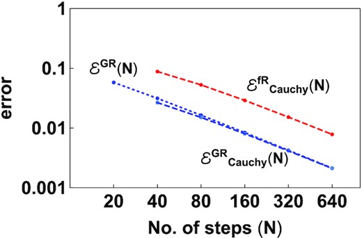
Convergence test of the algorithm. Comparison of successive approximations for evolution from a = 0.1 to a = 1 for profile 1a for the variable Δ. The algorithm was applied to a ΛCDM model with Φ = Ψ and an f(R) model with fR0 = −10−6.
