


ABSTRACT
Hot atmospheres pervading galaxy clusters, groups, and early-type galaxies are rich in metals, produced during epochs and diffused via processes that are still to be determined. While this enrichment has been routinely investigated in clusters, metals in lower mass systems are more challenging to probe with standard X-ray exposures and spectroscopy. In this paper, we focus on very deep XMM–Newton (∼350 ks) observations of NGC 1404, a massive elliptical galaxy experiencing ram-pressure stripping of its hot atmosphere while infalling towards the centre of the Fornax cluster, with the aim to derive abundances through its hot gas extent. Importantly, we report the existence of a new fitting bias – the ‘double Fe bias’ – leading to an underestimate of the Fe abundance when two thermal components cannot realistically model the complex temperature structure present in the outer atmosphere of the galaxy. Contrasting with the ‘metal conundrum’ seen in clusters, the Fe and Mg masses of NGC 1404 are measured 1–2 orders of magnitude below what stars and supernovae could have reasonably produced and released. In addition, we note the remarkable Solar abundance ratios of the galaxy’s halo, different from its stellar counterpart but similar to the chemical composition of the ICM of rich clusters. Completing the clusters regime, all these findings provide additional support towards a scenario of early enrichment, at play over two orders of magnitude in mass. A few peculiar and intriguing features, such as a possible double metal peak as well as an apparent ring of enhanced Si near the galaxy core, are also discussed.
1 INTRODUCTION
Over the two past decades, spatially resolved X-ray spectroscopy has considerably improved our knowledge of the growth of large-scale structures, such as galaxy clusters. The hot (107−8 K), X-ray emitting intracluster medium (ICM), falling into their deep gravitational well, constitutes in fact an unique way of probing the (thermo-) dynamics of most of clusters’ baryons, and to understand their assembly over cosmic times (for recent reviews, see e.g. Böhringer & Werner 2010; Simionescu et al. 2019a; Werner & Mernier 2020).
Beyond long-standing questions over its thermal and assembly history, the ICM also has intriguing chemical properties. In fact, it is known for hosting a substantial fraction of metals, which must have been synthesized and released by supernovae (SNe), before enriching the entire cluster volume (for recent reviews see e.g. Biffi, Mernier & Medvedev 2018; Mernier et al. 2018a). As clusters can retain all baryons permanently, the chemical elements they accumulate constitute a remarkable fossil record of the bulk enrichment of our Universe. More specifically: α-elements (e.g. O, Ne, Mg, Si, S) are mainly produced by core-collapse supernovae (SNcc), Fe-peak elements (e.g. Ca, Cr, Mn, Fe, Ni) are mainly produced by Type Ia supernovae (SNIa), while asymptotic giant branch (AGB) stars produce and release most of C and N elements (for a review, see e.g. Nomoto, Kobayashi & Tominaga 2013). As the aforementioned elements are all accessible via their K-shell (sometimes L-shell) emission lines in the energy band of the currently flying X-ray observatories, one can study the spatial distribution, relative ratios, and redshift-evolution of their abundances in order to better understand (i) the cosmic history of metals, (ii) their share and budget between cluster components, and (iii) their transport and diffusion mechanisms from sub-pc (SNe) to Mpc scales (clusters and groups).
Since the beginning of the XMM–Newton and Chandra era, many essential discoveries were done in this respect. Among them, one can certainly cite:
The presence of a central Fe peak in the most relaxed systems (e.g. De Grandi & Molendi 2001), with a very similar distribution for the other elements (e.g. de Plaa et al. 2006; Simionescu et al. 2009; Million et al. 2011; Mernier et al. 2017);
A remarkably uniform metallicity distribution in cluster outskirts, sometimes out to their virial radius (Werner et al. 2013; Urban et al. 2017; Ghizzardi et al. 2021);
A chemical composition very close to that of our own Solar System (de Plaa et al. 2007; de Grandi & Molendi 2009; Mernier et al. 2016a, b; Hitomi Collaboration et al. 2017; Mernier et al. 2018c; Simionescu et al. 2019b);
Redshift studies consistent with no evolutionary trend of abundances out to at least |$z$| ∼ 1.5 (though with non-negligible uncertainties; Ettori et al. 2015; McDonald et al. 2016; Mantz et al. 2017; Liu et al. 2018; Flores et al. 2021);
The ICM being too metal-rich compared to what could be reasonably produced by the stellar population in cluster galaxies, leading to a potentially serious conundrum in the metal budget at large scales (Arnaud et al. 1992; Bregman, Anderson & Dai 2010; Loewenstein 2013; Renzini & Andreon 2014).
Together with cosmological simulations (e.g. Biffi et al. 2017), these observations progressively gathered key evidence towards a scenario in which the ICM completed its enrichment at or beyond |$z$| ∼ 2–3 – coinciding with the main epoch of peak cosmic star formation history and maximal supermassive black hole activity (Madau & Dickinson 2014; Hickox & Alexander 2018) – with metals being thoroughly ejected and mixed at Mpc scales via feedback from active galactic nuclei (AGNs).
The case of lower mass systems, i.e. galaxy groups and early-type galaxies (ETGs), has been less studied and, consequently, less understood (for a recent review, see Gastaldello et al. 2021). The intragroup medium (IGrM) and the hot, X-ray emitting atmosphere pervading elliptical galaxies are also rich in metals, detected essentially via the Fe-L complex; however the latter remains essentially unresolved at current CCD spectral resolution, making the Fe abundance more sensitive to systematics. In addition, these systems are typically 1–2 order(s) of magnitude less bright than their cluster counterparts, hence requiring deeper observations. Interestingly, metal peaks are also observed in groups (e.g. Sun 2012; Mernier et al. 2017; Lovisari & Reiprich 2019) and, though less investigated than clusters, the metal mass in the IGrM tends to better agree with the available production from stellar sources (e.g. Renzini & Andreon 2014; Sasaki, Matsushita & Sato 2014). The case of these lower mass systems, however, is more challenging to interpret, as their shallower gravitational well (resulting in relatively stronger AGN feedback, competing with external gas accretion) prevents them from being considered as closed-box systems. Also, despite growing indications towards a chemical composition not so different between the ICM and the IGrM (Kim & Fabbiano 2004; Loewenstein & Davis 2010, 2012; Mernier et al. 2018c), the more extreme case of ETGs needs to be more thoroughly addressed. Ultimately, linking the chemical budget and history of ETGs (and groups) to that of clusters is absolutely essential to unify the enrichment picture at all extragalactic scales.
An excellent target to tackle these issues is NGC 1404 (FCC 219). This massive elliptical galaxy (12.7 × 10¹⁰ M⊙; Iodice et al. 2019) is falling towards the centre of the Fornax cluster (particularly its central dominant galaxy NGC 1399, a.k.a. FCC 213), and its relative proximity (less than 20 Mpc) allows its gas properties to be studied in great detail. Though likely at its second or third passage already (Sheardown et al. 2018), its infall makes it a textbook example of ram-pressure stripping at play between a galaxy’s hot atmosphere and its surrounding ICM (Machacek et al. 2005; Su et al. 2017b, a, c). The particular interaction of this ETG with the Fornax cluster makes its dynamics essentially restricted to (i) gas loss (via ram-pressure stripping) and (ii) a discontinuous interface (cold front) between the two media, in which Kelvin–Helmholtz instabilities may develop (depending on the gas viscosity and magnetic draping; Su et al. 2017a); however, it also prevents its hot atmosphere from experiencing substantial external accretion. Last but certainly not least, this galaxy does not have any known AGN activity (i.e. neither strong nuclear nor diffuse radio emission, nor X-ray cavities have been detected so far), and there are interesting indications of its atmosphere being rather turbulent compared with that of other ETGs (Pinto et al. 2015; Ogorzalek et al. 2017).
Thanks to its peculiar dynamics, NGC 1404 has benefited from deep Chandra exposures, so far mostly used for imaging purposes (Su et al. 2017b, a). Recent deep XMM–Newton observations were also conducted to derive high upper limits on its turbulence (Bambic et al. 2018). In both cases, however, the chemical enrichment aspect of its X-ray halo has not been addressed in detail. Accordingly, in this paper, we take advantage of these observations to probe the metal distribution of NGC 1404 as well as its chemical composition with unprecedented accuracy. The emphasis is put on XMM–Newton for its spectroscopic capabilities, via its three European Photon Imaging Cameras (EPIC; allowing spatial spectroscopy at moderate energy resolution) and its two Reflection Grating Spectrometers (RGS; allowing high resolution spectroscopy across a central detector strip). Nevertheless, we also show how data from the Advanced CCD Imaging Spectrometer (ACIS) onboard Chandra are nicely complementary in specific cases.
Throughout this paper, we assume a ΛCDM cosmology with H0 = 70 km s−1 Mpc−1, Ωm = 0.3, and |$\Omega _\Lambda = 0.7$|. We assume NGC 1404 to be at a distance of 18.79 Mpc (Tully, Courtois & Sorce 2016), for which 1 arcmin corresponds to 5.47 kpc. Its optical radii Re and R25 (respectively 2.3 kpc and 11.5 kpc; Sarzi et al. 2018) are fully covered by our spatially resolved analysis. Following Pinto et al. (2015), we adopt r500 = 0.61 Mpc. All the abundances are referred with respect to the proto-solar values of Lodders, Palme & Gail (2009, referred to as ‘Solar’ for simplicity). Unless stated otherwise, the error bars correspond to the 68 per cent confidence level.
2 DATA REDUCTION AND ANALYSIS
2.1 Chandra observations
Table 1 lists the 20 archival Chandra pointings with the ACIS-S or ACIS-I chips covering NGC 1404 and/or its immediate surroundings. We reduce all these data using the ciao (v4.11) analysis package as well as the calibration files of 2019 September (CALDB v4.8.4.1). Following the standard procedure, we reprocess the data reduction using the ciao task chandra_repro before filtering them from possible soft proton flares in the 0.5–7 keV band using the 2σ clipping setup of the task deflare. The images are then co-added and exposure-corrected in the 0.3–2 keV band (via the routine merge_obs), before we adaptively smooth the combined result (via the algorithm csmooth). The resulting flux map, shown in Fig. 1, reveals some exquisite features of the hot atmosphere of NGC 1404 during its interaction with the ambient ICM surrounding NGC 1399 (e.g. the well known cold front and ram-pressure tail; Machacek et al. 2005; Su et al. 2017b, a, c). We also carefully identify point-sources irrelevant to our analysis (either behind or belonging to NGC 1404), by using the task wavdetect. Finally, the raw spectra and their associated the response matrix files (RMF) and ancillary response files (ARF) are generated via the task specextract.
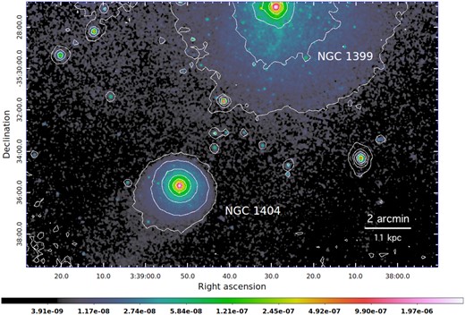
Adaptively smoothed, exposure-corrected flux map of NGC 1404 (and NGC 1399) observed from combined Chandra/ACIS observations in the 0.3–2 keV band. This mosaic includes ACIS observations that do not necessarily cover the immediate surroundings of NGC 1404 (see also Table 1). The white contours correspond to the background-, exposure-corrected XMM–Newton/EPIC counts (MOS 1 + MOS 2 + pn) in the same energy band.
List of XMM–Newton and Chandra observations used in this work. A fifth XMM–Netwon pointing (ObsID:0055140101) is not used here, as the position of NGC 1404 close to the detector edge (hence strongly impacting the PSF of the source) would have considerably complicated our analysis.
| Observatory | ObsID | Observation date | Raw exposure | Net exposure |
|---|---|---|---|---|
| (yyyy-mm–dd) | (ks) | (ks) | ||
| XMM–Newton | 0012830101 | 2001-06-27 | 29.2 | 6.3 |
| 0304940101 | 2005-07-30 | 55.0 | 28.4 | |
| 0400620101 | 2006-08-23 | 130.0 | 114.1 | |
| 0781350101a | 2016-12-29 | 134.3 | 126.7 | |
| Total | – | 348.5 | 275.5 | |
| Chandra | 240b | 2000-06-16 | 43.5 | 44.1 |
| (ACIS-S) | 319 | 2000-01-18 | 60.3 | 56.8 |
| 2389b | 2001-05-08 | 14.7 | 14.7 | |
| 2942 | 2003-02-13 | 30.0 | 29.6 | |
| 9530b | 2008-06-08 | 65.0 | 60.1 | |
| 9798 | 2007-12-24 | 18.3 | 18.3 | |
| 9799 | 2007-12-27 | 21.3 | 21.3 | |
| 14527 | 2013-07-01 | 27.8 | 27.8 | |
| 14529 | 2015-11-06 | 31.6 | 31.6 | |
| 16231 | 2014-10-20 | 60.5 | 60.5 | |
| 16232 | 2014-11-12 | 69.1 | 69.1 | |
| 16233 | 2014-11-09 | 98.8 | 98.8 | |
| 16639 | 2014-10-12 | 29.7 | 29.7 | |
| 17540 | 2016-04-02 | 28.5 | 28.5 | |
| 17541 | 2014-10-23 | 24.7 | 25.1 | |
| 17548 | 2014-11-11 | 48.2 | 48.2 | |
| 17549 | 2015-03-28 | 61.6 | 61.6 | |
| Chandra | 239 | 2000-01-19 | 3.6 | 3.6 |
| (ACIS-I) | 4172b | 2003-05-26 | 44.5 | 44.5 |
| 4174 | 2003-05-28 | 50.0 | 46.3 | |
| Totalc | – | 664.0 | 656.8 |
Note.a RGS data presented in this work are analysed from this pointing only. b These pointings do not cover the centre of NGC 1404 and, therefore, are used for imaging purposes only (Fig. 1). c Includes only observations covering NGC 1404 (hence suitable for spectroscopy analysis; see the text).
2.2 XMM–Newton observations
The bulk of this work relies on XMM–Newton observations of NGC 1404, as we aim to take advantage of the excellent spectral capabilities and effective area of its EPIC and RGS instruments. We use the four observations that are publicly available in the archive, as listed in Table 1, and reduce them using the XMM–Newton Science Analysis System (sas v17.0.0). The calibration files of 2019 January are used.
2.2.1 EPIC
Following the general prescription of Mernier et al. (2015), the MOS (i.e. MOS 1 and MOS 2) and pn data are pre-processed using the task emproc and epproc, respectively. We keep the single, double, triple, and quadruple events in the MOS data (pattern≤12) and restrict the pn data to single events only (pattern = 0). To minimize the detector contamination by soft protons emitted by solar flares, we use the sas task espfilt to define good time intervals (GTIs) that are then used to filter our data. Specifically, light curves in the 10–12 keV band are used to derive 100 s count rate histograms. Count rates exceeding 2σ from the mean of the best-fitting (Gaussian) distribution are then excluded from our GTIs. More accurate than selecting count rate thresholds arbitrarily, this 2σ clipping method is also repeated in the 0.3–2 keV band, as flares were reported at soft energies as well (De Luca & Molendi 2004). We also use the task edetect_chain to detect and further exclude point sources. Images and raw spectra are then extracted using the task evselect. A combined, exposure-corrected image (co-added with the task emosaic) focusing on the ram-pressure tail is shown in Fig. 2. The RMF and ARF are obtained using the tasks rmfgen and arfgen, respectively.
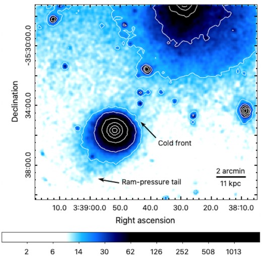
Exposure-corrected XMM–Newton/EPIC counts image of NGC 1404 in the 0.3–2 keV band, with its corresponding SB contours. The ram-pressure tail in the SE direction, as well as the NW merging cold front, are indicated.
2.2.2 RGS
Among the four available XMM–Newton pointings, only two (of 134 ks and 55 ks) are centred on NGC 1404 and are thus suitable for RGS analysis. Among these two, we choose to rely only on the RGS data available taken with the deepest XMM–Newton observation (ObsID:0781350101 – see Table 1). This choice is made for self-consistency and to avoid unnecessary difficulties in the analysis, since the two observations are made at different roll-angles and their central coordinates slightly differ as well. Such risk for extra systematic effects would be quite important in comparison to the low (≲20 per cent) statistics improvement expected from co-adding that second pointing.
The data are extracted and obtained following the same procedure as in Pinto et al. (2015) and Mernier et al. (2015), i.e. based on the sas task rgsproc. During the process, we also filter RGS 1 and RGS 2 data from flaring events using the same GTIs as for MOS 1 and MOS 2, respectively. We choose to include 90 per cent of the point spread function (PSF) along the cross-dispersion direction (xpsfincl = 90), which represents a spatial width of about 0.8 arcmin. This choice allows us to minimize the instrumental line broadening (due to the slit-less feature of the gratings – see Section 3) while keeping a large number of counts (thanks to the high central flux of the source combined with the deep exposure of our selected observation). We then combine the RGS 1 and RGS 2 spectral data and responses for each order separately using the spex task rgscombine. These combined spectra are fitted simultaneously for order 1 and 2.
2.3 Selected regions
As we discuss further in this paper, NGC 1404 and its chemical enrichment are interesting on many aspects. Fig. 3 summarizes the spatial locations that are considered in this analysis. These locations include (i) a box-shaped region covering the galaxy core, (ii) azimuthally averaged radial profiles, and (iii) 2D maps of the galaxy and its vicinity.
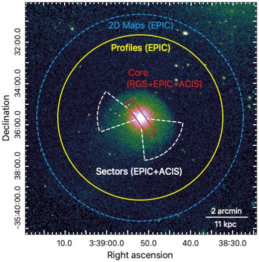
Zoomed-in Chandra/ACIS image of NGC 1404 (Fig. 1). The spectral extraction regions used in this work are indicated and their choice are further motivated in the text (Section 2.3). The central rectangular region (red) coincides with the RGS coverage of the deepest XMM–Newton observation, selected with ∼0.8 arcmin of cross-dispersion width.
The ‘core’ (i.e. central box) region is based on the extraction region of the deepest RGS pointing (Section 2.2.2). The box is defined such that its length direction is aligned with the RGS dispersion direction of the latter. Although this work relies essentially on the spectroscopic capabilities of the EPIC and RGS instruments onboard XMM–Newton, the remarkably deep net Chandra/ACIS exposures in the immediate vicinity of NGC 1404 (656.8 ks) offers the unique opportunity to compare the best-fitting properties obtained with each instrument within a common spectral region, hence to cross-check the consistency of our measurements. For each ACIS observation allowing so (see Table 1), we thus extract a spectrum corresponding to the same core region. Unlike RGS, which integrates photons over the entire field-of-view diameter along its dispersion direction, we choose to restrict the EPIC and ACIS core regions to the typical extent of the galaxy (i.e. 2 arcmin), in order to minimize the counts-over-background ratio on these CCD observations. To avoid further technical complication in the spectral analysis, we also restrict our core EPIC analysis to the two deepest XMM–Newton pointings only. Their dominant exposures (Table 1) make us confident that this has negligible effect on our final estimates (i.e. less than ∼15 per cent improvement on our statistics), without adding much information given the predominance of systematic over statistical uncertainties for deep pointings.
The ‘profiles’ regions consist of 10 EPIC concentric annuli centred on the galaxy’s X-ray emission peak and covering 4 arcmin of total radius. These annuli are defined with arbitrary outer limits at 16, 31, 46, 61, 80, 105, 140, 175, 205, and 240 arcsec, as the result of a good compromise between (i) reasonably high S/N ratio in each annulus (∼230 in external regions, up to ∼380 in the core) – translating into relative ΔFe/Fe uncertainties of 8–|$14{{\ \rm per\ cent}}$|, and (ii) delimiting regions of interest – in particular the merging cold front at 105 arcsec (∼10 kpc) from the core.
The 2D map is divided into 50 spatially independent EPIC cells, each having a (MOS + pn) constant S/N ratio of 200. The size and shape of the cells are obtained via the Weighted Voronoi Tesselation (WVT) binning method of Diehl & Statler (2006). We ensure that (i) the smallest cells (∼ 14 arcsec of diameter) remain larger than the typical PSF of the EPIC instruments (∼6 arcsec full width at half-maximum), (ii) the cells do not significantly overlap with the cold front, and (iii) all identified EPIC point sources were previously discarded from the map. In total, the map covers the whole ∼5 arcmin area surrounding the galaxy.
In addition, we define Eastern and Western sectors that are extracted in both ACIS and EPIC instruments (white dashed lines in Fig. 3). The reasons for analysing these additional two sectors and the motivation for their angle and extent are further developed in Section 5.
3 SPECTRAL ANALYSIS
The spectral analysis of our EPIC, RGS, and ACIS selected regions is performed via the spex fitting package (Kaastra, Mewe & Nieuwenhuijzen 1996) using the up-to-date Atomic Code and Tables (SPEXACT v3.06; Kaastra et al. 2020) and the ionization balance of Urdampilleta, Kaastra & Mehdipour (2017). Before performing the spectral fitting itself, we use the spex auxiliary tool trafo to convert the raw spectra, the RMFs, and the ARFs from the traditional OGIP format (respectively .pi, .rmf, and .arf) into spex-readable files.
The X-ray emission of NGC 1404 is modelled with successively one (1T), two (2T), and three (3T) collisionally ionized plasma components cie and one power-law po, all first redshifted and absorbed (red*[hot*[cie + ... + po]]) and set to a distance of 18.79 Mpc (Section 1). In the 3T case, we fix one temperature component to kTICM = 1.5 keV to model the emission from the surrounding ICM of the Fornax cluster. These choices are compared, justified, and discussed further in Section 4. The power law, with its photon index set to 1.6 (e.g. Su et al. 2017a), is aimed to reproduce the integrated X-ray emission from the galaxy’s low-mass X-ray binaries (LMXB). Although we model this component in all our selected annuli, we further verify its negligible contribution outside of the galaxy core (Section 4.2) and, therefore, fix it to zero in corresponding outer map cells. The redshift value is fixed to |$z$| = 0.00649 (Graham et al. 1998). The reference hydrogen column density of the absorbing hot model is nH = 1.57 × 1020 cm−2 (Willingale et al. 2013), which we allow to vary along a fixed grid within 0.51–2.51 × 1020 cm−2 as slight but significant offsets from the reference values are sometimes reported (e.g. Mernier et al. 2016a; de Plaa et al. 2017). The electron temperature of this same model is set to a negligible value of 0.5 eV in order to mimic absorption by a neutral gas, while its abundance parameters are all kept to the Solar value.
Our choice of the energy band to be considered depends evidently on the instrument. In the case of XMM–Newton EPIC, we chose 0.6–10 keV, while our Chandra ACIS spectra are fitted within 0.6–7 keV. In particular, we take care of avoiding setting the lower energy limit to 0.5 keV, as its proximity with the oxygen K-edge leads to erratic fitting and biased best-fitting estimates. Last but not least, we fit our RGS observations within 8–27 Å (roughly corresponding to 0.46–1.55 keV). Except the RGS spectra which are re-binned with a factor of 5 to reach 1/3 of the spectral resolution, we use the optimal binning method of Kaastra & Bleeker (2016) to analyse the EPIC and ACIS spectra. All fits are performed with C-statistics (Kaastra 2017).
Unless mentioned otherwise, the free parameters of our fits are (i) the emission measure1 of each cie component (Ygas, low, Ygas, high, and Ygas, ICM when relevant), (ii) the temperature of one or two cie components (kT1T for the 1T case; kTlow and kThigh for both the 2T and 3T cases), (iii) the emission measure of the po component (YLMXB), and (iv) specific abundance parameters (Mg, Si, S, and Fe for the EPIC and ACIS spectra; N, O, Ne, Mg, Fe, and Ni for the RGS spectra), assumed for each element to be the same in all cie components.2 In every case, all the other Z ≥ 6 abundances are tied to that of Fe. We stress the importance of coupling the O abundance in the EPIC and ACIS spectra to that of Fe in order to avoid critical biases in the fit. In fact, while the O line is essentially unresolved at CCD resolution, the high statistics of its corresponding spectral region forces the fit to reproduce its shape tightly, at the cost of incorrect estimates of other key features (e.g. temperature structure and/or abundances in the Fe-L complex).
3.1 RGS line broadening
3.2 Background treatment approaches
In extended sources, it is crucial to treat the background carefully, as it can significantly impact our measurements at larger radii.
As the RGS and ACIS data are mainly used to study the core region of NGC 1404, background effects from these two instruments are expected to be limited. Therefore, we follow individually their standard prescriptions by extracting the background from, respectively, (i) ACIS blank-sky observations processed and re-pointed using the ciao task blanksky, and (ii) RGS background templates of CCD 9 (via the sas task rgsproc), where presumably no source count is expected. We then rescale and subtract these background templates from their corresponding spectra.
The EPIC background deserves more careful attention, as we use these instruments also to explore the outer parts of the source. As detailed in Mernier et al. (2015), we model five well-known background components in our EPIC spectra; namely the Local Hot Bubble (LHB), the Galactic Thermal Emission (GTE), the Unresolved Point Sources (UPS), the residual Soft Protons (SP), and the Hard Particle (HP) background. The LHB and GTE are modelled, respectively, with an unabsorbed and absorbed cie component (kTLHB = 0.07 keV and kTGTE = 0.20 keV). The UPS is modelled with a power law of index ΓUPS = 1.41 (Moretti et al. 2003; De Luca & Molendi 2004). While these (foreground or background) components have an astrophysical origin, the SP and HP background components have an instrumental origin and, therefore, should not be folded by the ARF of the instruments. The SP component is modelled with a power law of a priori undetermined index (as it can vary between individual pointings and/or instruments) while the HP component is modelled with a broken power law and a series of Gaussian lines with values listed in Mernier et al. (2015). The normalizations and other a priori unkown parameters are first left free and determined over the entire field of view, then fixed and rescaled accordingly to the selected regions, taking the vignetting curves of each detector into account where appropriate.
4 RESULTS
4.1 Galaxy core
Besides its deep statistics, the very core of NGC 1404 has the advantage of being observed by (XMM–Newton and Chandra) CCD spectrometers and the RGS instrument. This provides an interesting opportunity not only to derive key thermal and chemical properties with unprecedented accuracy, but also to compare them between all these instruments (i.e. EPIC MOS, EPIC pn, RGS, and ACIS), with the aim to better understand their most recent cross-calibration (at least in this cool temperature regime).
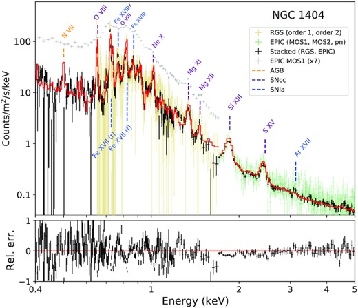
The RGS order 1 and 2 spectra, shown in Fig. 4 with a 3T modelling, exhibit a number of well-identified metal lines. We note, for instance, a clear signal at the expected N vii line energy, allowing us to measure its abundance with decent accuracy. Similarly, and unlike some other ETGs, the Mg xi and Mg xii lines as well as the Ne x line are prominent and well resolved. We note, however, the weak emissivity of the O vii lines, suggesting a small amount of cooling gas below typically kT ≲ 0.5 keV (e.g. Pinto et al. 2014). Despite the impressive resolving power of the instrument, its lower effective area translates into a less robust estimate of the continuum. While the absolute abundances have thus limited constraints, the relative X/Fe ratios do not directly depend on the equivalent width (hence on the continuum) of one line; therefore they can be measured accurately (Table 2; see also e.g. Mao et al. 2021). We also note from the RGS spectrum (Fig. 4) that the Fe xvii resonance line at 15 Å is affected by a significant optical depth, resulting in resonant scattering (see also Ogorzalek et al. 2017), in turn leading to partial suppression of its line flux. After re-fitting the RGS spectrum excluding this line, however, we find that the changes on the Fe abundance and X/Fe ratios are marginal (i.e. less than ∼5 per cent and ∼10 per cent, respectively – thus fully consistent with our statistical error bars).
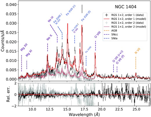
XMM–Newton RGS fit of the core of NGC 1404 (0.8 arcmin width, i.e. 90 per cent of the PSF). Both first and second orders are shown here. Prominent emission lines are labelled in orange, purple, or blue, depending on the stellar source of the concerned element (AGB, SNcc, or SNIa, respectively).
Best-fitting results for the core region of NGC 1404. The ACIS and EPIC extraction regions are chosen to coincide with the RGS extraction region (see the text and Fig. 3). f All abundances are estimated using full-band fits. n Abundances other than Fe are estimated using narrow-band fits.
| Parameter | ACISn | MOSn | pnn | EPIC (MOS + pn)f | RGSf |
|---|---|---|---|---|---|
| Ygas, low (1069 m−3) | 0.73 ± 0.12 | 1.53 ± 0.19 | 1.35 ± 0.17 | 1.44 ± 0.14 | 1.23 ± 0.19 |
| Ygas, high (1069 m−3) | 1.64 ± 0.12 | 2.05 ± 0.23 | 2.4 ± 0.3 | 2.17 ± 0.18 | 2.29 ± 0.18 |
| Ygas, ICM (1069 m−3) | 0.05 ± 0.03 | <0.016 | <0.018 | <0.009 | <0.06 |
| YLMXB (1069 m−3) | 0.492 ± 0.021 | (EPIC) | (EPIC) | 0.638 ± 0.017 | 2.14 ± 0.21 |
| kTlow (keV) | 0.484 ± 0.02 | 0.476 ± 0.016 | 0.450 ± 0.017 | 0.462 ± 0.012 | 0.38 ± 0.03 |
| kThigh (keV) | 0.723 ± 0.010 | 0.706 ± 0.012 | 0.690 ± 0.011 | 0.699 ± 0.008 | 0.664 ± 0.021 |
| Fe | 0.95 ± 0.06 | 0.74 ± 0.06 | 0.72 ± 0.07 | 0.74 ± 0.04 | 0.66 ± 0.14 |
| N/Fe | – | – | – | – | 2.7 ± 0.5 |
| O/Fe | – | – | – | – | 0.74 ± 0.06 |
| Ne/Fe | – | – | – | – | 1.14 ± 0.10 |
| Mg/Fe | 0.75 ± 0.06 | 1.07 ± 0.09 | 1.03 ± 0.10 | 1.03 ± 0.10 | 1.13 ± 0.12 |
| Si/Fe | 1.01 ± 0.12 | 1.33 ± 0.12 | 0.90 ± 0.09 | 1.22 ± 0.11 | – |
| S/Fe | |$0.9_{-0.5}^{+0.9}$| | 2.0 ± 0.3 | 0.43 ± 0.16 | 1.87 ± 0.20 | – |
| Ni/Fe | – | – | – | – | 2.2 ± 0.3 |
The opposite situation takes place in the EPIC spectra. As illustrated in Fig. 5, the moderate spectral resolution of the MOS 1, MOS 2 (hereafter, designated as ‘MOS’ when fitted simultaneously) and pn instruments is compensated by their large spectral window, allowing a proper continuum estimate – at least outside of the Fe-L complex. We also note that, whereas the flux of the hot gas emission dominates that of the other components by a factor of >20 in the 0.6–2 keV band, the LMXB component starts to dominate beyond ∼2 keV (with a 0.3–10 keV luminosity of 1.1 × 1040 erg s−1). The Si and, more importantly, the S abundance measurements are thus expected to be affected by the latter, if not perfectly modelled. The Mg abundances, however, are expected to be much more reliable. As we discuss further, the presence of fluorescent Al K α instrumental lines in the EPIC spectra may seriously bias Mg measurements in the case of dominant (particle) background contributions; however the very high S/N ratio prevents this issue in such a central region (Fig. 5). The same remarks apply to the ACIS spectra.
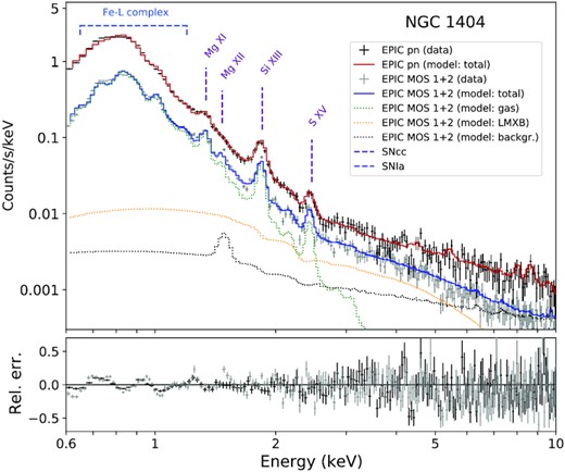
Combined XMM–Newton EPIC fit of the core of NGC 1404. The extraction region has been selected for the two deepest pointings to match that of RGS (0.8 arcmin width). Best-fitting models for the ICM emission (green), the LMXB component (yellow), and the (astrophysical and instrumental) background (black) are shown in dotted lines. For clarity, the spectral data of the MOS 1 and MOS 2 instruments have been stacked. Prominent emission lines/complexes are labelled in purple or blue, depending on the stellar source of the concerned element (SNcc, or SNIa, respectively).
One common practice on measuring metal abundances (and particularly their X/Fe ratios) in high-quality CCD spectra is to fit the latter over the full spectral band. A more conservative way is to perform the same fit within a narrow band, centred on the relevant emission line (i.e. 1–1.7 keV, 1.6–2.3 keV, 2.2–2.8 keV for Mg, Si, and S, respectively). These ‘narrow-band’ fits (in which the only free parameters are the relevant abundance and the total emission measure of the cie models5) have the advantage of accounting for subtle (yet non-negligible) miscalibration of the local effective area, which may have biased the estimate of the local continuum (hence of a few abundances) in the full-band fit (e.g. Mernier et al. 2015, 2016a; Simionescu et al. 2019b). For evident reasons, narrow-band fits can be performed on well-resolved lines only, and are thus not possible on Fe (which relies on the Fe-L complex at this temperature regime).
Fig. 6 and Table 2 compile and summarize the relevant best-fitting parameters and X/Fe abundance ratios obtained in this central region in the 3T case using these various instruments. These results are virtually identical to the 2T case, as Ygas, ICM is found to be negligible here. For comparison, results from both full-band and narrow-band fits are displayed in Fig. 6. On the other hand, in Table 2 we focus on ratios measured conservatively with narrow-band fits in each individual CCD instrument. Encouragingly, we find very similar (higher and lower) temperatures between all the instruments, with disagreements never exceeding ∼0.1 keV. The three XMM–Newton instruments also agree remarkably well (within 1σ) in terms of absolute Fe abundance, which is measured around 0.74 Solar. A slight but significant difference appears when considering ACIS, the latter measuring Fe almost 30 per cent higher than the RGS and EPIC measurements. This effect is related to the best-fitting Ygas, high and Ygas, low parameters which are measured somewhat lower in ACIS than in EPIC (Table 2).
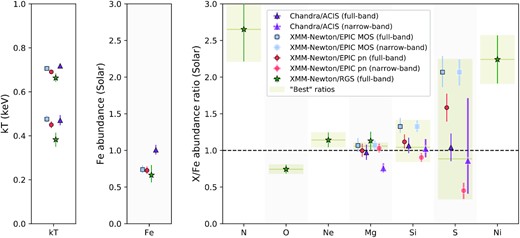
Best-fitting temperatures (kT), Fe abundances, and X/Fe abundance ratios obtained with XMM–Newton/EPIC, RGS, and ACIS within a rectangular region covering the RGS extraction region of the deepest XMM–Newton observation (see the text and Fig. 3). The MOS, pn, and ACIS measurements are obtained over full-band fits for kT and Fe and narrow-band fits for the abundance ratios (see the text).
On the other hand, the X/Fe ratios provide somewhat contrasted results. First, we note the excellent agreement of Mg/Fe – around 1 Solar – between all the XMM–Newton measurements (regardless of the instrument and of the fitting methodology assumed here). The ACIS narrow-band Mg/Fe ratio is measured somewhat lower (around 0.75 Solar); however we recover the agreement when the ACIS absolute Mg abundance is normalized over the preferred EPIC/RGS Fe abundance. This further suggests that ACIS tends to overestimate the absolute Fe abundance, while leaving the (absolute) Mg abundance properly measured. Secondly, we note a larger scatter in our Si/Fe measurements, though formally consistent with being Solar. The situation deteriorates when considering the S/Fe measurements, spanning between ∼0.3 and ∼2.3 Solar. The discrepancies found in these latter two ratios are not surprising, as the Si-K and S-K equivalent widths are likely to be significantly affected by the background and/or the LMXB component(s) (see above). While this clearly affects the reliability of the S abundance, we choose to consider Mg and Si (as well as their respective X/Fe ratios) in the rest of the analysis. Finally, we report the N/Fe, O/Fe, Ne/Fe, and Ni/Fe ratios measured with RGS only. These ratios, along with the ones mentioned above, are further discussed in Section 5.2.
Last but not least, we also aim to fit the RGS and the EPIC spectra all simultaneously, as shown in Fig. 7. Although this attempt leads to somewhat unstable fits (with e.g. difficulties to constrain two temperatures at the same time, given the imperfect calibration between the RGS and EPIC energy limits), we note that the measured X/Fe ratios are all formally consistent with our previous measurements. Beyond these numbers, this combined fit and its resulting figure may provide a useful glimpse (albeit at lower spectral resolution) of the spectral structure that will be routinely observed at this temperature regime by the next generation of X-ray micro-calorimeters onboard XRISM (XRISM Science Team 2020) and, on longer term, Athena (Barret et al. 2018).
Combined XMM–Newton RGS (1 & 2) + EPIC (MOS 1, MOS 2, & pn) fit of the core of NGC 1404. The EPIC extraction region has been selected to match that of RGS (0.8 arcmin width). In order to keep all spatial regions consistent, only the deepest pointing has been used for RGS, while the two deepest pointings have been selected for EPIC (see the text). For clarity, the spectral data have been stacked over the different EPIC and RGS instruments. Line labels are the same as in Figs 5 and 4.
4.2 Radial profiles
The most relevant best-fitting parameters derived from our nine concentric annuli (Section 3) are shown in Table 3 and Fig. 8. In the four panels of the figure, we also show (in green) the EPIC (MOS + pn) radial SB profiles.
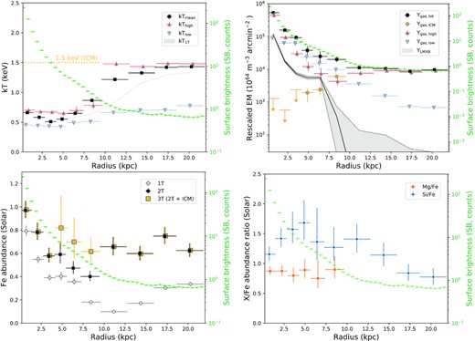
Radial profiles of NGC 1404, analysed with XMM–Newton/EPIC. In each plot, we also show the EPIC SB profile (green). Data points are slightly shifted along the x-axis for clarity. Top left-hand panel: Temperatures of the free gas components, and their weighted mean. The temperature of the surrounding ICM component, fixed to 1.5 keV, is also shown for clairty. Top right-hand panel: Emission measures (EM) for the different components (three hot gas components, one LMXB component), rescaled to their extracted area. The fixed value of the third thermal component, corresponding to the surrounding ICM, is also indicated (orange). Bottom left-hand panel: Fe abundance. Results for 1T, 2T, and 3T fits are shown separately and discussed in the text. Bottom right-hand panel: Mg/Fe and Si/Fe abundance ratios. The Mg and Si abundance parameters were fitted within a narrow energy band centred on their K-shell lines (see the text).
Best-fitting results for our (azimuthally averaged) radial profiles of NGC 1404, using the EPIC instruments. All parameters are derived using full-band fits of the EPIC (MOS + pn) instruments, except the Mg/Fe and Si/Fe ratios which include the conservative limits of (individual) MOS and pn narrow-band fits.
| Region | Ygas, low | Ygas, high | Ygas, ICM | YLMXB | kTlow | kThigh | Fe | Mg/Fe | Si/Fe |
|---|---|---|---|---|---|---|---|---|---|
| (kpc) | (1067 m−3) | (1067 m−3) | (1067 m−3) | (1067 m−3) | (keV) | (keV) | |||
| 0–1.5 | 20 ± 4 | 99 ± 9 | <0.3 | 25.7 ± 0.8 | 0.45 ± 0.03 | 0.701 ± 0.007 | 0.97 ± 0.08 | 0.87 ± 0.08 | 1.16 ± 0.13 |
| 1.5–2.8 | 58 ± 7 | 39 ± 5 | <0.4 | 10.7 ± 0.6 | 0.442 ± 0.016 | 0.677 ± 0.011 | 0.79 ± 0.08 | 0.87 ± 0.09 | 1.42 ± 0.17 |
| 2.8–4.2 | 63 ± 8 | 30 ± 7 | <2.4 | 7.5 ± 0.7 | 0.431 ± 0.013 | 0.668 ± 0.025 | 0.58 ± 0.07 | 0.80 ± 0.13 | 1.6 ± 0.3 |
| 4.2–5.6 | 33 ± 11 | 17 ± 7 | 2.7 ± 1.4 | 7.6 ± 0.9 | 0.424 ± 0.020 | 0.65 ± 0.04 | |$0.81_{-0.18}^{+0.28}$| | |$0.89_{-0.13}^{+0.18}$| | 1.7 ± 0.4 |
| 5.6–7.3 | 35 ± 16 | 17 ± 8 | 5.6 ± 1.8 | 12.9 ± 1.0 | 0.49 ± 0.04 | 0.69 ± 0.08 | |$0.70_{-0.14}^{+0.21}$| | |$0.75_{-0.16}^{+0.30}$| | |$1.4_{-0.3}^{+0.6}$| |
| 7.3–9.6 | 39 ± 12 | 17 ± 5 | 24.4 ± 2.3 | <3 | 0.51 ± 0.03 | 0.78 ± 0.09 | 0.62 ± 0.12 | |$0.89_{-0.15}^{+0.23}$| | |$1.27_{-0.22}^{+0.35}$| |
| 9.6–12.8 | 27 ± 3 | 57 ± 3 | – | <1.0 | 0.659 ± 0.009 | 1.48 ± 0.04 | 0.65 ± 0.09 | – | 1.4 ± 0.3 |
| 12.8–15.9 | 14.8 ± 1.0 | 87 ± 5 | – | <0.9 | 0.699 ± 0.020 | 1.43 ± 0.03 | 0.60 ± 0.06 | – | 1.14 ± 0.21 |
| 15.9–18.7 | 7.2 ± 0.5 | 80 ± 4 | – | <0.4 | 0.70 ± 0.03 | 1.48 ± 0.03 | 0.75 ± 0.08 | – | 0.84 ± 0.15 |
| 18.7–21.8 | 9.2 ± 1.0 | 123 ± 6 | – | <0.4 | 0.78 ± 0.04 | 1.48 ± 0.03 | 0.62 ± 0.06 | – | 0.77 ± 0.14 |
The top right-hand panel shows the emission measure of each modelled component. While no 1.5 keV gas is detected below ∼4 kpc, we see the relative contribution of Ygas, ICM steadily increasing towards the outer regions of the galaxy. Interestingly, we note that the relative predominance of a given (cool versus hotter) thermal component inverts twice across the whole profile. In fact, while the cooler component exceeds the hotter component by a factor of ≳2 within ∼4–10 kpc (with similar temperatures), the hotter components dominate by an order of magnitude beyond ∼13 kpc and within the innermost ∼1.5 kpc. Whereas the gas remains thus close to isothermal in the very core and in the ICM surrounding the galaxy, the intermediate regions show clear evidence of multi-temperature structure. As naturally expected, the total gas emission measure Ygas, tot, simply defined as the sum Ygas, low + Ygas, high + Ygas, ICM, follows well the SB profile when assuming a proper normalization factor between the two quantities. In addition, we also plot the derived emission measure of the LMXB component, YLMXB. Compared with Ygas, tot, this component drops faster within the first ∼3 kpc, then flattens out to ∼6.5 kpc, before vanishing outside of the galaxy’s SB as expected. It is not clear whether the intermediate flattening of the LMXB component is real or related to subtle fitting artefacts (e.g. intermediate thermal components); however we note that this component systematically lies a factor of ≳5 below the total hot gas component. This makes us confident that LMXBs affect our present results only weakly.
The bottom left-hand panel shows the Fe abundance as measured in our simultaneous MOS + pn fits successively in the 1T, 2T, and 3T cases. We have verified that, for each case, individual MOS and pn fits provide consistent results. The lower abundance (and different profile shape) measured with 1T compared to multitemperature modelling is expected: in fact, metallicities measured from CCD-resolution spectra are well known to be underestimated if the temperature structure is modelled too simplistically with one component only (the so-called ‘Fe bias’; see e.g. Buote & Canizares 1994; Buote 2000; Mernier et al. 2018a; Gastaldello et al. 2021). It is interesting to note (and, in fact, remind) that this bias occurs even when one gas component dominates the other by one order of magnitude (see the top right-hand panel). Much more surprising, however, is to find a significant Fe difference between the 2T and 3T cases within ∼4–10 kpc. This suggests that, at these intermediate radii where the ICM component competes with the galaxy’s atmosphere, modelling spectra with 2T is not realistic enough. This ‘double Fe bias’ is important to report as it significantly alters the shape of the Fe profile (particularly the apparent presence of a jump at ∼10 kpc) and its subsequent physical interpretations. The 3T profile appears to be centrally peaked, radially decreasing from ∼1 Solar in the very core down to ∼0.6 Solar outside of the galaxy and in the surrounding ICM. For consistency check, we verify that 2T and 3T fits provide virtually identical Fe abundances in the surrounding ICM.
Finally, the bottom right-hand panel shows the radial distribution of the Mg/Fe and Si/Fe ratios, using the narrow-band fits from MOS and pn individually. The MOS and pn results are then combined in each annulus. Whereas the Si abundance can be reliably measured out to large distances (despite a relative proximity with the Si K α line at ∼1.75 keV in the MOS instruments), the brightest instrumental line Al K α coincides in energy with the Mg-K lines (i.e. ∼1.5 keV) in both detectors, making outer Mg abundance measurements less reliable. In fact, outside the sixth annulus the source-to-background counts ratio in the 1.4–1.6 keV band drops below 1.5. For this reason, we choose to restrict our Mg/Fe measurements to the innermost ∼10 kpc. Although we note that the Mg/Fe ratios are on average somewhat lower than in the central box region (Section 4.1), their radial distribution through the galaxy extent is remarkably flat, in line with what is typically reported for more massive systems (e.g. Mernier et al. 2017). A more surprising result, however, is that the Si/Fe ratio appears much less uniform, with hints for an enhancement at intermediate radii and/or a central drop. This is further discussed in Sections 4.3 and 5.1.
4.3 Metal (and thermal) maps
In addition to the (azimuthally averaged) profiles described in the previous section, 2D spatial variations of the thermal and chemical properties of interest in NGC 1404 are investigated.
Fig. 9 focuses on the 2D thermal properties of the galaxy and its surroundings. In line with what is observed in our radial profiles, the higher temperature (top left-hand panel) shows important spatial variations between the ETG’s hot gas and the surrounding ICM. Interestingly, we note that this component becomes somewhat cooler along the ram-pressure tail. The lower temperature (top right-hand panel), on the other hand, remains more uniform across the full map extent (though with a slight decrease towards the centre) – again in agreement with our azimuthally averaged profiles. Combining these two temperatures (as well as kTICM in the inner ∼10 kpc cells), the mean temperature (bottom left-hand panel) reveals the dichotomy between the NGC 1404’s hot atmosphere and the Fornax ICM. In particular, we note little variation within the galaxy extent, while a clear temperature jump is seen at the interface of the NW merging cold front. The ram-pressure tail, somewhat cooler than its surroundings, is also clearly visible. Although comparable at first glance, this 3T map is not identical to its 1T counterpart (bottom right-hand panel). Similar to our radial analysis, we find that kT1T is underestimated in intermediate regions and we suspect this bias to be due to its multitemperature structure.
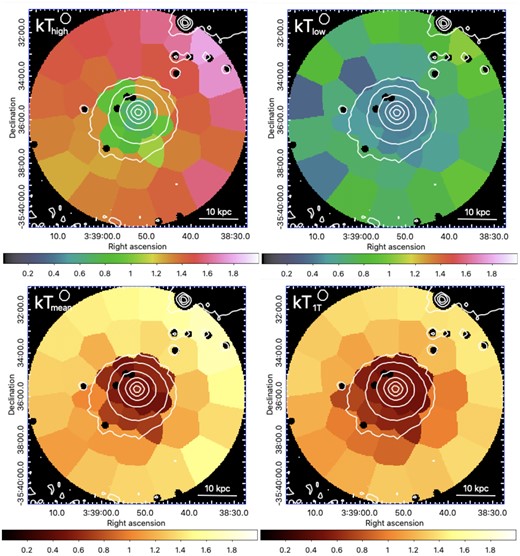
Temperature maps (in units of keV) obtained directly or indirectly from the EPIC fits (see the text). Top left-hand panel: Higher temperature (kThigh) measured with 3T fits (2T fits in the surrounding ICM). Top right-hand panel: Lower temperature (kTlow) for the same fits. Bottom left-hand panel: Mean temperature (kTmean) measured with 3T fits (2T fits in the surrounding ICM). Bottom right-hand panel: Temperature (kT1T) measured with 1T fits everywher on the map. The white contours are taken from the EPIC image and the cold front is approximately located on the NW edge of the outermost contour.
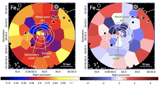
Fe abundance map (in Solar units) derived with the EPIC instruments using either 3T fits (left-hand panel) and its residuals compared to the azimuthally averaged profile (right-hand panel – see the text). The map has been colour-coded to emphasize cells with >1σ residuals. Noteworthy features are annotated on the figures.
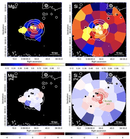
Abundance maps of Mg (top left-hand panel) and Si (top right-hand panel), and of the deviations (or residuals – see the text) of their ratios (X/Fe)res (bottom left-hand panel, bottom right-hand panel). The Si-rich arc discussed in the text is annotated on the bottom right-hand panel.
5 DISCUSSION
5.1 The peculiar metal distribution in and around NGC 1404
5.1.1 Central metal peak and ram-pressure stripping
The Fe distribution is centrally peaked – a feature that is commonly found in the hot gas of other (cool-core) galaxy groups and ETGs. This peak is better parametrized in Fig. 12, based on a series of Monte Carlo radial fits on the Fe profile, assuming possible values to be distributed within the 1σ uncertainties of the Fe abundance measurements.
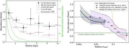
Left-hand panel: (Zoomed-in) Fe and Mg radial profiles of NGC 1404, compared with the X-ray (gas) and K band (2MASS; stars) SB profiles. In order to be compared in a consistent way, these two SB profiles are normalized to their respective peak value. For consistent comparison, the (normalized) square-root of the X-ray SB, tracing the gas density, is also shown. The grey curve corresponds to the middle quartile of a series of fits over the range of uncertainties of the Fe radial profile (see the text). Right-hand panel: Full Fe radial profile (with is lower, middle, and upper estimated quartiles) compared with the average radial profile of 21 galaxy groups and ETGs (CHEERS; Mernier et al. 2017). For consistent comparison, this average profile is also corrected from the most recent SPEXACT version (v3.06, see the text). The average uniform metallicity in cluster outskirts is also shown for comparison (Urban et al. 2017), as well as recent simulation results from Choi et al. (2020) including AGN feedback.
Zooming on the inner 10 kpc, (Fig. 12, left-hand panel), we notice that the Fe distribution is comparable to that of the gas density, inferred from taking the normalized square-root of the X-ray SB.6 However, it is clearly broader than the stellar distribution, as traced by the K-band luminosity of the galaxy (obtained publicly from the 2MASS survey), as well as its effective radius (Re ≃ 2.3 kpc; Sarzi et al. 2018). Both these comparisons are also found in other systems, in particular relaxed clusters (e.g. De Grandi et al. 2014). In line with the uniform Mg/Fe ratio (Fig. 8, bottom right-hand panel), the radial Mg profile is found to have a shape remarkably similar to that of Fe.
Comparing our present Fe profile with the 21 groups/ETGs of the CHEERS sample, NGC 1404 shows a rather unusual metal distribution. Indeed, although the surrounding ICM has its Fe abundance comparable to that seen in other systems at the same distance, the central Fe peak of NGC 1404 seems narrower and flattens at small radii. This difference seems independent of spectral codes, holding also when correcting the previous CHEERS measurements to the latest SPEXACT version (v3.06 – following the method described in Mernier et al. 2020). The most immediate interpretation for such a difference is the peculiar environmental conditions of this galaxy. Likely, ram-pressure stripping – seen in earlier works (e.g. Machacek et al. 2005; Su et al. 2017b, a) and through the cooler SE gas tail in Fig. 9 has significantly contributed to erode metals from its initial central build-up. If true, this picture provides strong evidence that ram-pressure stripping is an effective mechanism to eject metals from individual galaxies into their cluster environment. Interestingly, NGC 1404 is also known for showing credible signs of higher turbulence than in most (if not all) other studied systems (Pinto et al. 2015; Ogorzalek et al. 2017), despite its lack of recent AGN activity. A high turbulence in NGC 1404 would be expected to stir metals, hence to broaden its central metal core. That intuitive picture contrasts instead with the remarkably narrow Fe peak reported here. This suggests that mixing of metals through their hot atmospheres is considerably more sensitive to ram-pressure stripping rather than to turbulence and small-scale gas motions. This does not preclude at all, however, that in more common conditions the kinetic feedback mode of central AGNs dominates the metal distribution process, for instance via jets and buoyant bubbles displacing directly central low-entropy metal-rich gas to higher altitudes (Simionescu et al. 2008; Kirkpatrick, McNamara & Cavagnolo 2011; Kirkpatrick & McNamara 2015). This would, in fact, naturally connect the narrow extent of the central peak with the absence of (visible) AGN feedback in this galaxy (see also Rebusco et al. 2006).
We also note that, like in earlier work (e.g. Mernier et al. 2017), the central Fe and Mg peaks are significantly lower than those predicted by the state-of-the-art simulations in ETGs; e.g. the MACER simulations (Pellegrini et al. 2020) and the MrAGN runs of Choi et al. (2020). The precise origin of these disagreements still has to be determined, but should be (at least partly) related to the complex subgrid physics at play here.
5.1.2 Two central metal peaks?
In addition to the central metal peak, the residual maps from Figs 10 and 11 show a secondary peak that is marginally detected with >1.2σ. Intriguingly, this peak is not associated with any particular feature in X-ray/radio/optical SB, nor with particular gas temperature structure. If real, interpreting this peak is not easy, however the least unlikely scenario would be that of a localized region of star formation.
Assuming a line-of-sight velocity of 522 km s−1 for NGC 1404 towards NGC 1399 (Su et al. 2017b) and, very roughly, that this offset peak is widely entrained by such velocity via ram-pressure stripping, we estimate that metals must have been released less than ∼6 Myr in this region before being dislocated. Comparing this time-scale with the (∼one order of magnitude) longer time-scale for massive stars to eject metals via SNcc explosions, it comes that such a hypothetical star-forming region should have remained active and largely visible in blue optical bands. Since, again, no counterpart is visible in the optical nor radio bands, the such star-forming region seems implausible. One should keep in mind, however, the rough assumptions considered here: non-negligible gas viscosity and/or relative steadiness of the inner parts of the galaxy may very well keep this secondary peak essentially intact.
5.1.3 Metal-poor arc inside the cold front?
While our (3T) azimuthally averaged Fe profile favours a smooth decrease from ∼1 to ∼0.6 Solar, our corresponding 2D analysis shows a significant metal-poor arc that is found to lie inside the NW cold front. This finding contrasts with other merging/sloshing systems, in which metallicity drops to lower values outside their associated cold front (e.g. Simionescu et al. 2010; Ghizzardi, De Grandi & Molendi 2014; Werner et al. 2016; Urdampilleta et al. 2019). To our knowledge, this is the first time that such opposite situation is reported.
This peculiar feature is difficult to interpret. One possibility is that the gas outside the central metal peak was initially enriched at ∼0.3 Solar and remained so until the galaxy began to interact with the Fornax ICM. If the ICM and NGC 1404’s atmosphere do not mix well across the merging cold front (e.g. shielded by magnetic draping, whereas in the opposite direction the tail helps mixing the gas efficiently), a metal-poor arc inside the cold front may have survived from the galaxy’s motion through the ICM. In a similar scenario, the ICM surrounding NGC 1404 may have compressed (but not mixed with) the whole metal gradient of the system when interacting with the Fornax cluster. These two possibilities, however, are not supported by numerical simulations, as the latter typically predict the emergence of gas motions inside the cold front as well (Heinz et al. 2003; Markevitch & Vikhlinin 2007).
Another – perhaps more likely – possibility is that the metal-poor arc is not real. Extending the ‘double Fe bias’ case discussed in Section 4.2, projection effects along the cold front region may very well result in a temperature distribution more complex than our simple 3T assumption. In turn, our improved modelling approach may still not be sufficient to provide fully unbiased Fe abundances. Although deriving information from even more complicated multitemperature modelling is challenging at this temperature regime, we note that this cold-front region constitutes a target of choice for future observation campaigns at higher spectral resolution; particularly with XRISM/Resolve and, at improved spatial resolution, Athena/X-IFU.
5.1.4 The (dissimilar) Mg and Si spatial distributions
Our results show that Mg follows Fe remarkably well locally in the hot gas of NGC 1404. Given that Fe and Mg originate from different SNe types (respectively, SNIa and SNcc) with, in principle, different enrichment histories and time delays, finding a spatially uniform Mg/Fe distribution suggests that these two channels had enriched the hot atmosphere of NGC 1404 early on, well before the dynamics of the system affected the distribution of these elements (via e.g. ram-pressure and internal motions). This picture, discussed more extensively in the next sections, can be naturally put into the context of the early enrichment scenario for clusters and groups in general, as such spatial uniformity of α/Fe ratios has been already reported in the ICM of more massive systems and interpreted in a similar manner (de Plaa et al. 2006; Simionescu et al. 2009, 2015; Ezer et al. 2017; Mernier et al. 2017).
More surprising is the Si-rich arc, corresponding to a radial increase of the Si/Fe ratio to super-Solar levels reported between ∼2 and 7 kpc (Fig. 8, bottom right-hand panel). To investigate this further, we have refitted spectra from EPIC MOS, EPIC pn, and ACIS sectors extending in the E and W directions, as shown in Fig. 3. Interestingly, we find a super-Solar enhancement at >1σ in both directions with similar trends for the three instruments independently, meaning that the Si-rich arc might as well be azimuthally independent. This Si-rich ring, confirmed independently by three instruments and two fitting methodologies (i.e. narrow-band in the EPIC profiles, full-band in the EPIC maps and the EPIC/ACIS sectors discussed here), cannot be attributed to instrumental effects only. In fact, the instrumental Si K α line at ∼1.75 keV is present in MOS (and likely in ACIS as well) but not in pn.
Such a finding is difficult to explain within any standard SNIa/SNcc enrichment scenario. Indeed, since both Mg and Si are presumably synthesized by SNcc (with a non-negligible SNIa contribution for Si; e.g. Mernier et al. 2016b; Simionescu et al. 2019b), one would naturally expect to see similar spatial distributions for the two elements. If a ring of enhanced SNcc enrichment was indeed in place in NGC 1404, such a feature should appear at least as prominently in the Mg/Fe ratio. Alternative astrophysical explanations remain sparse. One could speculate either towards a separate enrichment channel for Si (possibly occurring at a distinct epoch, leading to segregated motion/diffusion histories in the hot gas), or towards selective interactions of Si between two phases – for instance an efficient central depletion of Si into dust, as already proposed to explain metal drops in other systems (e.g. Panagoulia, Sanders & Fabian 2015; Mernier et al. 2017; Lakhchaura, Mernier & Werner 2019; Liu, Zhai & Tozzi 2019). We note, however, the remarkably low dust mass estimates that are reported for NGC 1404 so far (Skibba et al. 2011; Rémy-Ruyer et al. 2014).
Interestingly, this is not the first time that a non-flat Mg/Si trend is reported: using deep Chandra observations, Million et al. (2011) found a centrally peaked Si/Fe distribution in the core of M 87, together with a flatter Mg/Fe profile. While the authors interpret their results as an incomplete spectral modelling, in our case we rather speculate on a fitting bias related to the complex temperature structure below the cold front region. If, as discussed before, the absolute Fe abundance is indeed biased low in that region (and so is the Mg abundance, as its line is not entirely dissociated to the Fe-L complex), the Si/Fe may be overestimated. Unlike the Fe-L complex, the Si-K line lies in fact in a band that is likely less sensitive to subtle multitemperature effects. Whether this Si-rich arc/ring is genuine or not will be likely verified by future high-resolution observations (Athena/X-IFU and, to some extent, XRISM/Resolve).
5.2 The chemical composition of NGC 1404
In Fig. 13, we compare the abundance ratios obtained conservatively in this work (black stars) with earlier relevant results from the literature. We find an excellent agreement with the abundance pattern of the average ICM (yellow boxes – the 44 nearby systems of the CHEERS sample, though strongly weighted towards clusters; Mernier et al. 2018c). In the same figure, our (gas-phase) ratios are also compared with corresponding stellar ratios from previous work: (i) the stellar ratios as measured with SDSS in a sample of ETGs (Conroy, Graves & van Dokkum 2014);7 (ii) the stellar Mg/Fe ratio from MUSE observations of NGC 1404 within the Fornax3D project (Iodice et al. 2019, blue limits tracing two aperture radii). Overall, it comes that the galaxy’s stellar population and its hot atmosphere have a different chemical composition, with a clear α/Fe enhancement in the former.
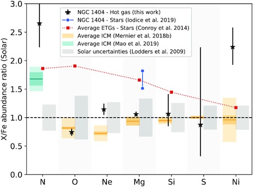
Comparison between the abundance ratios presented in this work (core region) and other measurements, namely: (i) the stellar Mg/Fe ratio derived by Iodice et al. (2019) for the same galaxy (delimited by the measurements within 0.5 Re and beyond 0.65 arcmin); (ii) average stellar X/Fe ratios for a sample of ETGs with similar stellar mass (Conroy et al. 2014, log M* = 11.07); and (iii) average X/Fe measured in hot atmospheres of the CHEERS sample (44 clusters, groups, and ETGs; Mernier et al. 2018c) and in a subsample of eight systems (mostly ETGs; Mao et al. 2019). For comparison we also show the Solar uncertainties (Lodders et al. 2009).
Three ratios deserve further attention, as they do not formally agree with the ICM abundance pattern.
The Ni/Fe ratio is measured to be super-Solar, at variance with the up-to-date ICM estimates (Hitomi Collaboration 2017; Mernier et al. 2018c; Simionescu et al. 2019b). However, unlike the hotter ICM – in which Ni is measured via its K-shell transitions around 7.8 keV, the cooler temperature regime of ETGs makes Ni measurements possible only via the Ni xix transitions that are drowned into the Fe-L complex. Even at the RGS energy resolution, these lines are broadened instrumentally and cannot be fully resolved. For instance, the most prominent Ni line in our RGS spectra (at ∼14.1Å) is blended with the Fe xviii line (Fig. 4), the latter accounting for ∼95 per cent of the total flux at this wavelength range. Thus, the Ni/Fe best-fitting abundance shown here predominantly reflects subtle fitting adjustments in our RGS spectra (due to e.g. imperfect calibration or instrumental broadening), and therefore should be interpreted with extreme caution.
The N/Fe ratio is measured >3σ higher than its Solar value. Unlike Ni, the main N line at ETG-like temperatures is well resolved (N vii at ∼25 Å), hence its abundance measurement should be robust. In fact, super-Solar N/Fe ratios are a rather common feature to hot atmospheres, as already observed in other sources (e.g. the Centaurus cluster – Sanders et al. 2008; NGC 4636 – Werner et al. 2009) and in stacked samples as well (Sanders & Fabian 2011; Mao et al. 2019). The traditional interpretation is that N is released by AGB stars, thus independently of the SNIa and SNcc channels responsible for the enrichment of all the other probed elements. Interestingly, these ratios are at first order consistent with the typical stellar N/Fe ratios of ETGs of similar masses. This may suggest that, unlike the early SNIa/SNcc enrichment discussed above and further, AGB stars constitute a still ongoing (and thus fully decoupled) channel of metal production and release.
The Ne/Fe ratio agrees well with its Solar value, but is somewhat in tension with (in fact, higher than) previous ICM measurements. An interesting explanation may be the difference of temperature structure between the cool-core ICM and the hot atmosphere of NGC 1404. Whereas the former undergoes strong temperature gradients – likely resulting in a complex (projected) temperature distribution, the latter remains essentially isothermal in its very core (Section 4.2). This difference is important because hotter temperatures naturally boost the emissivity of Fe xxi and Fe xxii lines within 12–13 Å, making the Ne X line undistinguishable from those. Consequently, the Ne abundance is degenerate with the relative amount of hot versus cool gas, and both parameters cannot be well disentangled in RGS spectra of cool-core systems. As this is not the case here, our Ne/Fe ratio can be considered as better constrained and more reliable.8 Even better: assuming the Ne/Fe does not change (much) from system to system, our present ratio can be used as a reliable reference to be assumed in all future X-ray cluster/group studies. In turn, fixing Ne/Fe to ∼1.13 (or Ne/O to ∼1.54 in RGS spectra) could be used to alleviate the above degeneracy and better constrain the temperature structure in other systems.
5.3 Can the stellar population of NGC 1404 produce the metals of its hot gas?
Whereas the mass of metals observed in the ICM and that available from galaxy stellar populations have been already investigated in clusters (e.g. De Grandi et al. 2004; Simionescu et al. 2009, Ghizzardi et al. 2021), such budgets have not been quantified yet, to our knowledge, in the case of ETGs, particularly with low gas accretion and little AGN feedback. Although not isolated, NGC 1404 is an excellent candidate for such a case, as its rapid motion towards NGC 1399 prevents it from accreting external metals.
Fig. 14 shows our estimates of Mgas(< R), as well as MFe(< R) and MMg(< R) as ‘pure’ products of SNIa and SNcc, respectively (Si being produced by both channels). Evidently, accounting for the surrounding ICM beyond the cold front radius leads to a monotonic increase of all masses. Restricting our estimates to the gas extent of the galaxy (9.6 kpc), we find a total gas mass of Mgas = (6.9 ± 0.5) × 108 M⊙ as well as Fe and Mg masses of MFe = (6.2 ± 0.8) × 10 5 M⊙ and MMg = (3.0 ± 0.4) × 10 5 M⊙.

Encircled X-ray gas and metal (Fe and Mg) masses integrated within a given (azimuthally averaged) distance from the centre of NGC 1404. The solid and dashed curves indicate, respectively, the fully integrated and excess masses. The vertical line segments, coded with corresponding colours, indicate our estimated ranges of metals produced by SNIa and by stellar winds (see the text). The dotted vertical line corresponds to the radius within which the gas is assumed to have not interacted yet with the Fornax cluster (see Fig. 8, bottom left-hand panel).
In addition to the classical enclosed metal masses defined above, we are also interested in estimating the enclosed metal mass excess, MX, exc(< R), i.e. the metal mass of the central peak alone (subtracting the ‘flat’ abundance from the ‘total’ abundance profile). This is done easily by replacing X(r) with Xexc(r) = X(r) − X0 in equations (5) and (6), with X0 adopted here as the lowest abundance value found in the radial profile of element X. Also shown in Fig. 14, these Fe and Mg excess masses are, respectively, MFe, exc = (9 ± 5) × 10 4 M⊙ and |$M_\mathrm{Mg, exc} = (4.8_{-3.0}^{+4.8}) \times 10^4$| M⊙.
First, let us compare these metal masses with those reasonably produced by SNIa through the galaxy’s lifetime. Assuming the SNIa rate of Maoz & Graur (2017) for cluster galaxies (|$N_\mathrm{Ia}/M_* = 5.4 \times 10^{-3}~\mathrm{M}_\odot ^{-1}$|), the stellar mass of NGC 1404 (12.7 × 10¹⁰ M⊙) provides 6.9 × 10⁸ SNIa explosions. Using the SNIa yields from Seitenzahl et al. (2013), and depending on the assumed yield model, this translates into ejected masses of (2.4–7.6) × 108 M⊙ and (0.3–3.2) × 107 M⊙ for Fe and Mg, respectively. Although it is interesting to note that these SNIa-driven masses can largely account for both the Fe and the Mg observed masses, the large difference between the Fe and Mg ejecta produced by SNIa (by more than one order of magnitude) does not reflect the factor ∼2 difference between the observed masses of these two elements. Unless the escape (and/or depletion) fraction of Fe and Mg is for some reason highly segregated, a full SNIa origin for all the metals in NGC 1404 is thus highly unlikely.
Unlike SNIa, deriving metal masses produced by SNcc through the galaxy’s history is difficult as it strongly depends on its star formation history. Quantifying the latter is challenging, although like other massive ETGs NGC 1404 had likely undergone a short and brief star formation peak around |$z$| ∼ 3 (Thomas et al. 2010; Yates et al. 2013, see also our discussion in the next section). It is interesting to note, none the less, the absence of current star formation measured by MUSE in NGC 1404 (Iodice et al. 2019). The observed 1.4 GHz radio power of (1.03 ± 0.15) × 1019 W Hz−1 (Grossová et al. 2022) in the core of the galaxy could be explained by star formation that is three times lower than the FUV inferred estimate of (3.58 ± 0.04) × 10−2 M⊙ yr−1. Assuming this rate to be constant since |$z$| ∼ 3 along with a Salpeter IMF, negligible metal mass from SNcc contribution is expected during this recent epoch.
5.4 The chemical history of NGC 1404
In the previous sections, we have (i) compared the abundances in the hot atmosphere of NGC 1404 with those of other astrophysical sources, and (ii) compared the (Fe and Mg) observed metal masses with those expected from their stellar populations. In this last section, we discuss jointly all these findings with the attempt to derive a plausible chemical history for this particular galaxy.
Interpreting the remarkable similarity between the X/Fe ratios derived in the hot halo of NGC 1404 and in the ICM of rich clusters, the chemical composition of hot atmospheres does not depend on the mass of the system over nearly two orders of magnitude in mass. Our aforementioned core analysis essentially probes the central metal peak. Given the particular position and stripping motion of the galaxy within the Fornax ICM, this peak is directly associated to NGC 1404 itself, since it reflects metals that may have been either recently produced by its stellar population, or retained on to the galaxy for a long time; but certainly not accreted recently. On the other hand, the abundance pattern of NGC 1404’s atmosphere is clearly distinct from that of its (current) stellar population. The traditional interpretation for enhanced stellar α/Fe ratios in massive galaxies such as NGC 1404, is that they are the direct signature of the galaxy’s star formation history (see discussions in e.g. Thomas et al. 2010; Johansson, Thomas & Maraston 2012; Yates et al. 2013; Conroy et al. 2014; Simionescu et al. 2019b). Typically, massive ETGs undergo ‘downsizing’, i.e. an early, brief, and intense star formation episode that shuts down quickly after its onset. Consequently, the metal content of their stellar generations is predominantly locked with material from early SNcc enrichment – i.e. mostly α-elements. On the contrary, a significant fraction of SNIa explode later on, and their (mostly Fe-peak) material should end up in higher proportions into ETGs’ surrounding atmosphere. These initial considerations lead to three possible gas-phase enrichment scenarios.
First is the scenario of an ongoing enrichment, coming essentially from both delayed SNIa (Fe-peak elements) and stellar winds from the current stellar population (α-elements), and with no recent contribution from SNcc. As seen in Section 5.3, stellar winds and SNIa could have largely produced metals within this whole galaxy’s hot atmosphere. Moreover, such an ongoing enrichment would naturally explain the gas metal peak surrounding the bulk of its stellar population. This scenario, however, fails to explain the Solar gas-phase X/Fe ratios, as it would require a nearly perfect compensation between stellar winds and SNIa enrichment products to reproduce exactly this abundance pattern. Unless a remarkable fine-tune is at play over two orders of magnitude in mass, it also seems difficult to unify this picture with that of the ICM enrichment (which exhibits very similar abundances and ratios, and which is thought to have completed beyond |$z$| ∼ 2; e.g. Biffi et al. 2018; Mernier et al. 2018a).
A second, more likely scenario is that of an early enrichment, having started as early as the downsizing epoch of NGC 1404 (likely |$z$| ∼ 3) and completed no much later – around |$z$| ∼ 2. In such a scenario, both the stellar and the hot gas abundances are independently locked in time and do not further evolve. The main sources of this early enrichment would then be SNcc, prompt SNIa, and (to some extent) early stellar winds. Since this scenario is clearly favoured in the case of the ICM enrichment, a conciliation between ETGs and clusters scales arises naturally. It would also explain the remarkably Solar chemical composition found at all radii in these two types of systems (though we remind our surprising finding on Si/Fe in Section 5.1). Although difficult to quantify accurately, restricting our estimates from Section 5.3 to the 2 < |$z$| < 3 epoch only provides stellar wind and SNIa metal masses that can still comfortably account for the observed ones (e.g. in excess of a factor of ≳5 even for stellar winds).
A third, no less interesting possibility would be that of metals being present in the hot gas even before the star formation episode, hence likely also before the gas started to get heated to X-ray temperatures. This pre-enrichment scenario would then enrich the (not yet virialized) galaxy’s atmosphere via SNe explosions from early (probably metal-poor) stars, hence having very little to do with the current stellar population of NGC 1404. Extended to (massive) galaxies in general, such a scenario would have more profound consequences in our general considerations of the cosmic history and cycle of metals. It would have the advantage to unify the ICM and ETGs enrichment in an even more natural way than the early enrichment scenario, as simulations indeed predict a substantial amount of metals to have enriched clusters before |$z$| ∼ 3 (Biffi et al. 2017). It would also fit with the most natural explanation to the metal conundrum mentioned in Section 5.3, in the sense that the metal content of hot atmospheres at all scales would have very little to do with their associated stellar population (see e.g. Blackwell, Bregman & Snowden 2021). However, such a pre-enrichment scenario would hardly explain the narrow metal peak present in the core of NGC 1404, and would ignore the whole content of metals produced more recently which, in one way or another, must be present in its galactic atmosphere.
As discussed above, the early enrichment – and, to some extent, the pre-enrichment – scenarios are favoured to explain the chemical history of NGC 1404. No matter the scenario, however, the metal budget of this particular galaxy remains difficult to fully capture. Indeed, following our estimates in Section 5.3, a dominant fraction of metals that should have been released by (past and ongoing) stellar winds and SNIa is missing in our X-ray observations. It is evident that a substantial amount of these metals had probably left the galaxy and enriched the Fornax ICM – which is qualitatively in line with the efficiency of ram-pressure stripping to enrich its surroundings (Section 5.1, especially after a second passage in the cluster; Sheardown et al. 2018). The surprise, however, is that no chemical signature of stellar winds nor recent SNIa (via, respectively, enhanced or low α/Fe ratios) is found in the hot gas. On the opposite end of massive clusters, we may therefore be facing an ‘inverse metal conundrum’, in which the bulk of gas-phase metals are missing. It is interesting to note that these two condundra might (at least partly) compensate for each other: if these metals missing from individual ETGs are actually accreted on to associated clusters, the metal budget of the Universe may be less problematic than previously thought.
Clearly, probing metal budgets in other ETGs and massive clusters will be essential to further understand the complete cycle of metals at these large scales. In this respect, spatially resolved high-resolution spectroscopy onboard the future missions XRISM (XRISM Science Team 2020) and Athena (Barret et al. 2018) will be crucial.
6 CONCLUSIONS
In this paper, we have taken advantage of deep XMM–Newton (276 ks) and Chandra (657 ks) observations of the elliptical galaxy NGC 1404, to probe the chemical content of its hot atmosphere with unprecedented details. Plunging toward the centre of the Fornax cluster likely for the second or third time (Sheardown et al. 2018), this galaxy with no visible AGN feedback is known to exhibit a merging cold front at the interface of its atmosphere with the surrounding cluster medium, as well as an X-ray gas tail induced by ram-pressure stripping (e.g. Machacek et al. 2005; Su et al. 2017b, a). Following a careful spectral modelling, the Fe, Si, and Mg abundances were measured independently in the core region of the galaxy using the EPIC MOS, EPIC pn, RGS, and ACIS instruments. Similarly, we have also investigated the spatial distribution of these elements (both radially and in 2D maps) using the EPIC instruments. Our results are summarized as follows.
Measured through their X/Fe abundance ratios, the chemical composition of the central region is remarkably consistent with that of the hot gas of galaxy clusters, and with that of our Solar System (the only exception being the supersolar N/Fe ratio, likely originating from AGB stars). This pattern, however, differs from the stellar abundance ratios measured either at similar stellar mass bin (Conroy et al. 2014), or directly in NGC 1404 using MUSE (Iodice et al. 2019). We also note that the Ne/Fe ratio, measured robustly here, can be useful to better constrain the multiphaseness of the gas, which is otherwise hardly accessible in the (often unresolved) shape of the Fe-L complex.
We find a central metal peak significantly narrower than what is typically found in other ETGs and galaxy groups. This may suggest that ram-pressure stripping is an effective process to erode metal peaks in galaxies and eventually dilute elements in the surrounding ICM.
We report a new fitting bias, namely the ‘double Fe bias’, where even a two-temperature modelling leads to an underestimate of the Fe abundance in the case of complicated temperature structures. Taking a three-temperature modelling into account, we find for the first time a region of lower metallicity inside the NW merging cold front. Since such a metal-poor structure would be difficult to explain within conventional scenarios, we suspect that the abovementioned bias remains at play in this complex region.
Unlike the remarkably flat Mg/Fe distribution across the galaxy extent (in line with observations of the hotter ICM/IGrM), we measure a significant increase of the Si/Fe ratio ∼3–10 kpc away from the core. This trend is seen independently in EPIC MOS, EPIC pn, and ACIS, hence demonstrating that this is not an instrumental bias. This Si-rich ring is difficult to interpret, though it might either reveal complex transfer mechanisms between different phases of the ISM, or relate to the double Fe bias.
The mass of metals estimated in the hot gas phase of NGC 1404 (MFe ≃ 6 × 10⁵ M⊙; MMg ≃ 3 × 10⁵ M⊙) is found to be 1–2 orders of magnitude lower than the mass of metals expelled by SNIa and stellar winds since |$z$| ∼ 3. Beyond the fact that both sources of enrichment could have largely produced these metals (though the ICM and stellar X/Fe ratios do not favour a sole one), we are witnessing an inverse metal conundrum, in which too many metals should have been produced compared to what is currently seen. Nevertheless, the most plausible chemical history for NGC 1404 is that of an early enrichment (or even pre-enrichment), in which the bulk of metals produced by NGC 1404 had left the galaxy (and enriched the Fornax cluster) more than 10 Gyr ago, via ancient episode of AGN feedback and/or ram-pressure stripping.
This work shows the importance of multiwavelength studies to probe metals in (massive) galaxies at all phases. Future campaigns will be essential in the short-term future to obtain a full coherent picture of the chemical enrichment history, as well as its metal transportation mechanisms from sub-pc scales out to the largest (gravitationally bound) structures of our Universe.
ACKNOWLEDGEMENTS
The authors thank the anonymous referee for insightful comments that helped us to improve this paper. FM thanks Hiroki Akamatsu, Ena Choi, Jelle de Plaa, Simona Ghizzardi, Jelle Kaastra, Anwesh Majumder, Lýdia Štofanova, Remco van der Burg, Michael Wise, Xioaoyuan Zhang, and Zhenlin Zhu for fruitful discussions and/or complementary data. NW and RG are supported by the GACR grant 21-13491X. AS is supported by the Women In Science Excel (WISE) programme of the Netherlands Organisation for Scientific Research (NWO), and acknowledges the World Premier Research Center Initiative (WPI) and the Kavli IPMU for the continued hospitality. This work is based on observations obtained with XMM–Newton, an ESA science mission with instruments and contributions directly funded by ESA member states and the USA (NASA). The scientific results reported in this article are based in part on data obtained from the Chandra Data Archive. SRON is supported financially by NWO.
DATA AVAILABILITY
The original data presented in this article are publicly available from the XMM–Newton Science Archive (https://nxsa.esac.esa.int/nxsa-web/) and in the Chandra X-ray Center (https://cda.harvard.edu/chaser/). The respective XMM–Newton and Chandra data are reduced with the sas (https://www.cosmos.esa.int/web/xmm-newton/sas) and ciao softwares (https://cxc.cfa.harvard.edu/ciao) and further analysed spectrally with the spex fitting package (https://www.sron.nl/astrophysics-spex). Additional derived data products can be obtained from the main author upon request.
Footnotes
In spex, the emission measure is defined as Y = ∫nenpdV, where ne and np are respectively the electron and proton densities, integrated over the entire source emitting volume.
This assumption is admittedly simplified, and may not reflect the specific enrichment level of each component. High-resolution spectroscopy offered by future microcalorimeter instruments will enable us to alleviate this constraint. Meanwhile, the impact of this assumption on our present results is expected to be very limited given the radially uniform abundances found in regions of multitemperature gas (Section 4.2).
See the XMM–Newton Users Handbook.
See the spex reference manual.
Throughout this study, narrow-band fits are performed after coupling Ygas, high to Ygas, low, using the normalization derived from its corresponding broad-band fit. This way, we ensure that the total emission measure is fitted locally with one parameter only, avoiding fitting degeneracies.
Although this comparison needs to be taken with caution (as, in addition ot the continuum, the SB also includes a non-negligible fraction of metal line emission), we remind the good correspondence between Ygas, tot and the X-ray SB (Fig. 8 top left-hand panel).
NGC 1404 is in fact measured with M* = 1.3 × 10¹¹ M⊙ (Iodice et al. 2019), i.e. close to the highest stellar mass bin of the SDSS sample (red data points on the figure).
As a quantitative example: for an NGC 1404-like gas (i.e. kT = 0.7 keV), SPEXACT v3.06 predicts the Ne X line emissivity alone to be more than 3 times higher than the sum of the abovementioned Fe xxi and Fe xxii lines. For a kT = 1 keV gas, this ratio dramatically drops to 0.4.
REFERENCES
Author notes
ESA Research Fellow.
