


ABSTRACT
The interacting dark energy (IDE) model, which considers the interaction between dark energy and dark matter, provides a natural mechanism to alleviate the coincidence problem and can also relieve the observational tensions under the ΛCDM model. Previous studies have put constraints on IDE models by observations of cosmic expansion history, cosmic microwave background, and large-scale structures. However, these data are not yet enough to distinguish IDE models from ΛCDM effectively. Because the non-linear structure formation contains rich cosmological information, it can provide additional means to differentiate alternative models. In this paper, based on a set of N-body simulations for IDE models, we investigate the formation histories and properties of dark matter haloes and compare with their ΛCDM counterparts. For the model with dark matter decaying into dark energy and the parameters being the best-fitting values from previous constraints, the structure formation is markedly slowed down, and the haloes have systematically lower mass, looser internal structure, higher spin, and anisotropy. This is inconsistent with the observed structure formation, and thus this model can be safely ruled out from the perspective of non-linear structure formation. Moreover, we find that the ratio of halo concentrations between IDE and ΛCDM counterparts depends sensitively on the interaction parameter and is independent of halo mass. This can act as a powerful probe to constrain IDE models. Our results concretely demonstrate that the interaction of the two dark components can affect the halo formation considerably, and therefore the constraints from non-linear structures are indispensable.
1 INTRODUCTION
The cosmological constant-cold dark matter (ΛCDM) model, which built on the framework of general relativity and the hypotheses of dark energy and dark matter, is widely accepted so far as the standard cosmological model. It provides us physical scenarios of the evolution of Universe and the structure formation therein, which are supported by most of the cosmological observations today.
However, ΛCDM is still not the ultimate description for our Universe. From the theoretical aspect, the physical nature of dark energy and dark matter is not yet fully understood. There are long-standing fine-tuning and coincidence problems for the cosmological constant (Weinberg 1989; Zlatev, Wang & Steinhardt 1999). Observationally, the ΛCDM model can explain cosmic large-scale structures nicely but confronts acute problems at the dwarf-galaxy scale, namely the well-known missing satellites, core-cusp, and too-big-to-fail problems (see Bullock & Boylan-Kolchin 2017, for a review). In recent years, with the rapid observational developments, a few inconsistencies between different observations under ΛCDM have emerged and become increasingly significant. The most notable one is the H0 tension with the Hubble constant H0 derived from Planck cosmic microwave background (CMB) observations ∼5σ away from the ones measured from standard candles and the lensing time delay observations (Riess et al. 2019; Riess 2020; Wong et al. 2020). The other less significant one is the S8 tension where there is a 1−2σ discordance between the value of S8 = σ8(Ωm)0.5 constrained from Planck CMB and that from weak lensing measurements (Hikage et al. 2019; Hildebrandt et al. 2020; Amon et al. 2021; Asgari et al. 2021).
Given the problems, different non-standard cosmological scenarios have been proposed. Among them, the interacting dark energy (IDE) models have been regarded as physically well-motivated ones. In this framework, the two dark components that dominate the current evolution of the Universe are not independent but interact with each other. Thus, their densities coevolve, giving rise to a natural explanation for the coincidence problem (Amendola 2000; Amendola & Quercellini 2003; Pavón & Zimdahl 2005; Amendola, Tsujikawa & Sami 2006; Olivares, Atrio-Barandela & Pavón 2006; Böhmer et al. 2008; Chen, Wang & Jing 2008; Del Campo, Herrera & Pavón 2008). Furthermore, it has been testified that the IDE model with appropriate parameters is also effective to relieve the discordances under a ΛCDM framework that are mentioned before (Ferreira et al. 2017; An, Feng & Wang 2018). There have been extensive studies for IDE models, both from theoretical aspects (He, Wang & Abdalla 2009a; He, Wang & Jing 2009b; He et al. 2010; D’Amico, Hamill & Kaloper 2016) and from observational constraints (Costa et al. 2017; Zhang et al. 2019; Cheng et al. 2020; Kang 2021). See Wang et al. (2016) and Bolotin et al. (2015) for detailed reviews of IDE models.
It is noted that the current constraints on IDE models are mainly from cosmic expansion history, CMB, and the structure formation on large scales. Their effects on non-linear structure formation have not been fully investigated. Physically, the interaction between dark energy and dark matter induces their densities change in addition to that due to cosmic expansion. Furthermore, the accelerating force on dark matter particles is also altered. We therefore expect that the non-linear structure formation, in particular, the properties of dark matter haloes, can be considerably different in IDE models in comparison with their ΛCDM counterparts and thus can provide valuable information in constraining IDE models. The non-linear matter power spectra of IDE models have been studied in the recent years (Baldi 2011, 2012; Casas et al. 2016). In Carlesi et al. (2014a) and Carlesi et al. (2014b), they analysed the properties of dark matter haloes in different cosmic web environments at redshift z = 0 from hydrodynamical simulations of coupled and uncoupled quintessence models. The gas properties in clusters of galaxies were also investigated. Their findings show that the differences of halo properties, such as the spin and the concentration, between their considered models depend sensitively on the surrounding environment of haloes. The initial attempt to study the halo evolution in the coupled dark sector model was done in Jibrail, Elahi & Lewis (2020). However, the details of halo formation history and its properties are still lacking study.
Recently, a fully self-consistent N-body simulation pipeline for IDE models, ME-GADGET, was developed by Zhang et al. (2018), which enables us to trace the non-linear structure formation in IDE models accurately. Therefore, in this paper, based on a set of simulations from ME-GADGET, we analyse systematically the formation history and properties of dark matter haloes in IDE models, including mass function, density profile, spin, and shape.
The paper is organized as follows. We first introduce the phenomenological IDE models (Section 2.1) and our N-body simulations (Section 2.2) and then we describe the dark matter halo catalogues used in this study (Section 2.3). We present our results in Section 3. Summary and discussions are presented in Section 4.
2 METHODS
2.1 Phenomenological IDE models
IDE models that have been studied.
| Model | Q | wd |
|---|---|---|
| IDE1 | |$3\mathcal {H}\xi _{2}\rho _{\mathrm{d}}$| | −1 < wd < −1/3 |
| IDE2 | |$3\mathcal {H}\xi _{2}\rho _{\mathrm{d}}$| | wd < −1 |
| IDE3 | |$3\mathcal {H}\xi _{1}\rho _{\mathrm{c}}$| | wd < −1 |
| IDE4 | |$3\mathcal {H}\xi (\rho _{\mathrm{d}}+\rho _{\mathrm{c}})$| | wd < −1 |
In Costa et al. (2017), constraints on the models in Table 1 are derived using Planck CMB, BOSS BAO, Type Ia supernova and Hubble constant observations. While tight constraints are obtained for IDE3 and IDE4, only weak ones are achievable for IDE1 and IDE2. This is because the interactions in IDE1 and IDE2 are proportional to dark energy density, which came to be dominant only recently. Such an interaction has weak impacts on CMB anisotropy and cosmic expansion history and thus cannot be tightly constrained from the corresponding observations. However, the non-linear structure formation in these two models can be significantly different from that of ΛCDM model. Therefore, tighter constraints on IDE1 and IDE2 are expected by employing probes related to non-linear structures, such as the abundance of clusters of galaxies and weak lensing peak statistics. This is the motivation of our study here. Based on a set of IDE N-body simulations, we will perform systematic analyses on the non-linear structure formation in different models.
2.2 N-body simulations for IDE models
To generate self-consistent initial conditions, we first use the capacity constrained Voronoi tessellation method (Liao 2018; Zhang et al. 2021) to produce a uniform and isotropic particle distribution. We then modify the camb code (Lewis & Bridle 2002) to calculate the linear matter power spectra for IDE models and use the 2LPTic code (Crocce, Pueblas & Scoccimarro 2006) to generate the initial perturbed position and velocity for the particles. See Zhang et al. (2018) for details.
In our studies here, we consider five sets of simulations, ΛCDM, IDE1, IDE2, IDE1′, and IDE2′. The cosmological parameters adopted are shown in Table 2. The ones for the ΛCDM simulation are consistent with the Planck 2015 results (Planck Collaboration XIII 2016). The IDE1 and the IDE2 employ the best-fitting parameters constrained by Costa et al. (2017). We note that for utilizing the redshift space distortion (RSD) data into constraints on IDE models, consistent treatments using IDE templates to extract RSD information from galaxy redshift-space distributions are needed. These are still lacking in the current RSD analyses. We therefore choose to use the fitting parameters in table 4 and table 5 of Costa et al. (2017) for IDE1 and IDE2, respectively, derived from Planck CMB + BAO + SNIa + H0 without RSD. Additionally, we run two more IDE simulations, IDE1′ and IDE2′, with their parameters chosen to be the midpoint values between ΛCDM and best-fitting IDE1 and IDE2, respectively, which are well within the allowed parameter ranges from Costa et al. (2017).
Cosmological parameters for ΛCDM and IDE simulations. The ΛCDM parameters are from the Planck 2015 results (Planck Collaboration XIII 2016), while the parameters for IDE1 and IDE2 are the best-fitting values from the constraints using Planck CMB + BAO + SNIa + H0 by Costa et al. (2017). For the IDE1′ and IDE2′, their parameters are chosen to be at the midpoints between ΛCDM and the corresponding best-fitting IDE models.
| Parameter | ΛCDM | IDE1 | IDE2 | IDE1′ | IDE2′ |
|---|---|---|---|---|---|
| ln (1010As) | 3.094 | 3.099 | 3.097 | 3.0965 | 3.0955 |
| ns | 0.9645 | 0.9645 | 0.9643 | 0.9645 | 0.9644 |
| wd | −1 | −0.9191 | −1.088 | −0.95955 | −1.044 |
| ξ2 | 0 | −0.1107 | 0.05219 | −0.05535 | 0.026095 |
| h | 0.6727 | 0.6818 | 0.6835 | 0.67725 | 0.6808 |
| Ωd | 0.6844 | 0.7817 | 0.6631 | 0.7345 | 0.6769 |
| Ωm | 0.3156 | 0.2182 | 0.3368 | 0.2654 | 0.3230 |
| Ωr | 0 | 0.0001 | 0.0001 | 0.0001 | 0.0001 |
Each simulation evolves 5123 particles from z = 127 to 0 in a periodic box with a side length of 100 h−1 Mpc. Each simulation has 139 outputs in total, and the time interval for snapshots is ∼0.1 Gyr. The comoving gravitational softening length used in our simulations is 4 h−1 kpc, which is ∼1/50 of the mean inter-particle separation.
The particle mass in the ΛCDM simulation is 6.53 × 10⁸ h−1 M⊙. For IDE models, the particle mass is changing with time due to the interaction between dark energy and dark matter. Fig. 1 shows the particle mass versus redshift in different simulations, where the upper horizontal axis is the corresponding cosmic time in ΛCDM. For IDE1, dark matter decays into dark energy and, thus, the particle mass decreases from 6.25 × 10⁸ h−1 M⊙ at z = 127 to 4.51 × 10⁸ h−1 M⊙ at z = 0. For IDE2, the energy flows from dark energy into dark matter, and the particle mass increases from 6.27 × 10⁸ h−1 M⊙ to 6.96 × 10⁸ h−1 M⊙. Similar trends are seen for IDE1′ and IDE2′, but the changes are milder because of the smaller values of |ξ2|.
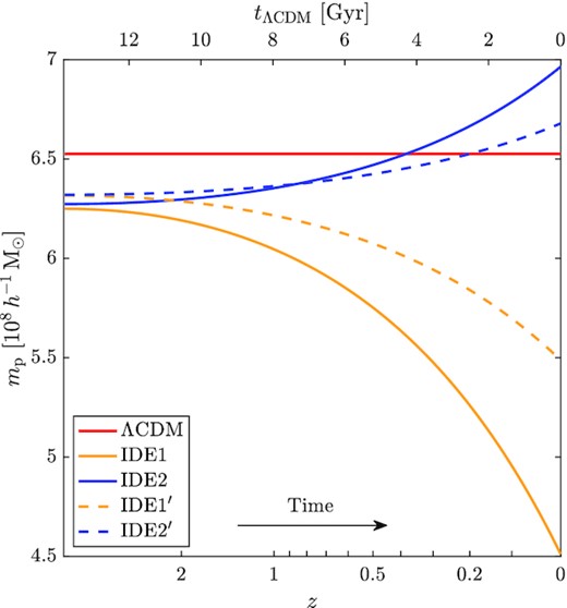
Evolution of particle masses in ΛCDM (red), IDE1 (yellow solid), IDE2 (blue solid), IDE1′ (yellow dashed), and IDE2′ (blue dashed) simulations. The lower horizontal axis shows the redshift, while the upper horizontal axis gives the corresponding looking-back time in ΛCDM.
We have used the same random seed to generate the initial conditions for the five simulations and, therefore, are able to conduct direct comparisons of the large-scale structures. Fig. 2 presents the cosmic matter density distributions of different scales at z = 0 from our simulations. From the top panels, we can see that the large-scale structures (≳ 10 h−1 Mpc) in IDE and ΛCDM models are fairly similar. However, when we zoom into smaller scales as shown in the middle and bottom panels, we can clearly see that the IDE1 (IDE2) structures tend to have lower (higher) central peak densities comparing to the ΛCDM counterparts. This illustrates that the differences between IDE and ΛCDM models are more enhanced at small-scale virialized structures, and it hints us that studying and quantifying the halo properties at low redshifts in IDE models can help to put tighter constraints on these models.
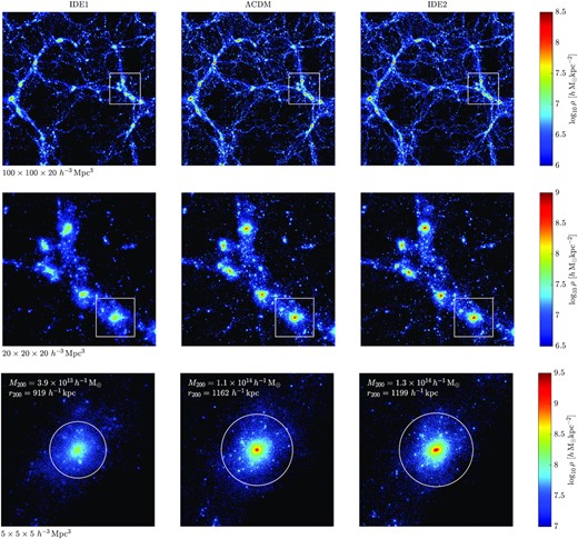
Contrasts on the z = 0 cosmic structures in IDE1 (left column), ΛCDM (middle column), and IDE2 (right column) models at different scales. Top row: 2D projections of the matter density distribution of a simulation slice with a side length of 100 h−1 Mpc and a thickness of 20 h−1 Mpc. Middle row: zoom-in plots of the high-density regions that are marked with the white squares in the top panels. Bottom row: zoom-in plots of a ΛCDM halo and its IDE counterparts that are marked with the white squares in the middle panels. The white circles in the bottom panels mark the halo virial radii r200. In each panel, the projected density is shown in logarithmic scale, and the colour bar for each row is shown on the right.
2.3 Dark matter halo catalogues
Based on the snapshot outputs of the ΛCDM, IDE1, IDE2, IDE1′, and IDE2′ simulations, we construct different dark matter halo samples for analyses, namely ALL, MATCH, and TRACE samples. Fig. 3 summarizes our construction pipeline considering the ΛCDM, IDE1, and IDE2 models as an illustration. We describe in detail the steps in this section. The same procedures are also performed parallelly for the case of IDE1′ and IDE2′.
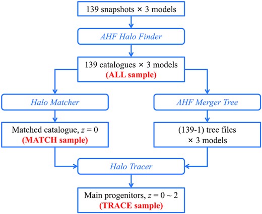
The pipeline to generate the ALL, MATCH, and TRACE halo samples based on the ΛCDM, IDE1, and IDE2 simulations.
2.3.1 ALL sample
We employ the AHF halo finder (Gill, Knebe & Gibson 2004; Knollmann & Knebe 2009), which works based on the spherical overdensity algorithm, to identify dark matter haloes from simulation snapshot outputs. We adopt the centre-of-mass position as the halo centre and define the halo virial radius, r200, as the radius within which the mean density is 200 times the cosmic matter density, ρm(z), at the corresponding redshift. For IDE models, we modify the related calculations in the ahf code to take into account the time evolution of the cosmic mean matter density (equation 5). We run the modified ahf code for all snapshots of the ΛCDM, IDE1, and IDE2 simulations from which 139 × 3 dark matter halo catalogues are obtained; we refer to them as ALL sample hereafter. The minimum particle number used in our halo identification is 50. However, to estimate the halo properties robustly, unless otherwise specified, we use only haloes with M200 > 1011 h−1 M⊙ (i.e. those that have at least ∼154 particles in the ΛCDM simulation) in our analyses.
2.3.2 MATCH sample
Specifically, for all z = 0 haloes that are more massive than 1011 h−1 M⊙ in the ALL sample, we match the ΛCDM haloes with IDE1 and IDE2 haloes, respectively, and keep only those haloes that have both IDE1 and IDE2 counterparts. These triplets serve as our initial matched halo sample. Then, the following selections are carried out:
Haloes in the IDE1 model have systematically lower masses than their ΛCDM counterparts, which will be shown in Section 3. To ensure the completeness of the matched sample, we therefore consider only the ΛCDM haloes with M200 ≥ 1012 h−1 M⊙ so that their counterparts in IDE models are all more massive than 1011 h−1 M⊙.
Because of the mass resolution limitation of our simulations, we mainly focus on the properties of host haloes in this study without analysing subhaloes. Thus, we remove a halo triplet from the initial matched sample if any of the three counterparts is a subhalo.
We pick out the halo triplets that have both |$\mathcal {M}_{\Lambda \mathrm{CDM-IDE1}}$| and |$\mathcal {M}_{\Lambda \mathrm{CDM-IDE2}}$| greater than 0.25. From the definition of the merit function, |$\mathcal {M}_{\mathrm{AB}}\gt 0.25$| means that at least half of the particles in halo A (or halo B) are common particles.
After applying the selections above, out of 4174 ΛCDM host haloes more massive than 1012 h−1 M⊙ at z = 0, there are 3763 ones that have reliable counterparts in both IDE1 and IDE2 simulations. They form the MATCH sample. The bottom row of Fig. 2 shows an example of a ΛCDM halo and its IDE counterparts.
2.3.3 TRACE sample
To study the halo formation history, we use the ahf Merger Tree code to construct the merger trees for all z = 0 haloes in the MATCH sample. Specifically, for a target halo in a certain snapshot, the ahf Merger Tree code searches for its progenitors in the previous adjacent snapshot by cross-matching halo particle IDs. If a candidate halo in the previous adjacent snapshot shares at least 10 common particles with the target halo, it is included as one of the progenitors of the target halo. The main progenitor is defined as the one that has the maximum merit function with the target halo.
To construct stable trees, the ahf Merger Tree code has the function to skip snapshot(s) when a halo is going through complicated environment and to cope with temporary large fluctuation in mass (see Srisawat et al. 2013, for more discussions). In this study, we require that if a target halo cannot find any progenitor in the adjacent snapshot or the mass ratio between the target halo and the progenitor candidate is larger than 2, the code will ignore this snapshot and continue to search for the credible progenitors in high-redshift snapshots.
In total, there are 3010 halo triplets at z = 0 from the MATCH sample whose merging histories can be traced back to z > 2 in all three models. We name them as the TRACE sample.
3 RESULTS
With the halo catalogues described above, we study the abundance, formation history, and internal properties of dark matter haloes in the IDE models and compare them with the ΛCDM counterparts. We note that the five models considered here do not have exactly the same H0 value, but the differences are small (i.e. |$\lt 2{{\ \rm per\ cent}}$|, see Table 2). We therefore use the conventional units of h−1 M⊙ and h−1 Mpc ( h−1 kpc) for mass and length in model comparisons and ignore the differences in H0.
3.1 Halo mass function
We first analyse the halo mass function, i.e. the comoving number density of dark matter haloes as a function of halo mass and redshift, n(M, z), for different models. As one of the most important quantities describing the non-linear structure formation, the halo mass function carries rich cosmological information and is the foundation to extract cosmological parameter constraints from observations of galaxy cluster number counts (Allen, Evrard & Mantz 2011; Abbott et al. 2020) and weak lensing peak statistics (Hamana, Takada & Yoshida 2004; Fan, Shan & Liu 2010). It also plays an essential role in building halo models (Cooray & Sheth 2002; Skibba & Sheth 2009) and the semi-analytic models of galaxy formation (Conroy, Wechsler & Kravtsov 2006).
For ΛCDM model, there have been extensive studies on the halo mass function (e.g. Press & Schechter 1974; Bond et al. 1991; Jenkins et al. 2001; Sheth, Mo & Tormen 2001; Reed et al. 2003; Tinker et al. 2008; Watson et al. 2013). In the IDE framework, He et al. (2009b) calculated the linear growth of perturbations, and subsequently He et al. (2010) studied the spherical collapse systems.
Here, we analyse the halo mass functions of different models based on the ALL sample, as shown in Fig. 4 for ΛCDM, IDE1, and IDE2. In order to investigate the evolution, besides the halo mass functions at z = 0 (right-hand panel), we also measure the results at z = 1 (left-hand panel) when the dark energy–dark matter interactions are still weak. At z = 1, both IDE models produce systematically less haloes than ΛCDM with the ratio of ∼0.76 and ∼0.87 for IDE1 and IDE2, respectively. This is mainly because of the lower ρm(z) at high redshift for the two models than that of ΛCDM (see Fig. 1 and equation 5).
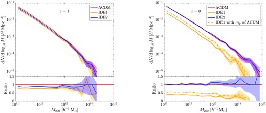
Halo mass functions at z = 1 (left) and z = 0 (right) in ΛCDM (red), IDE1 (yellow solid), and IDE2 (blue) models, respectively. The upper panels show the differential halo mass functions, while the lower panels show the ratios with respect to ΛCDM. The shaded region associated with each line represents the Poisson error. In the right-hand panel, the yellow dashed lines plot the rescaled IDE1 halo mass function (see the text for detailed discussions).
At z = 0, we see that the halo mass function of IDE1 model is markedly lower than that of ΛCDM over the whole considered mass range, and the difference increases at the high-mass end. For M200 ≈ 1011 h−1 M⊙, the ratio between IDE1 and ΛCDM is ∼0.41, while for M200 = 1014 h−1 M⊙, the ratio reduces to ∼0.23. For the considered IDE models, the interaction between dark energy and dark matter is proportional to the dark energy density. When dark energy becomes a dominant component at lower redshift, the interaction gets stronger. For IDE1, dark matter then decays into dark energy more effectively, which suppresses the growth of dark matter structures and even reduces the halo mass (see Section 3.2 for detailed discussions). We therefore observe a significantly lower halo mass function at z = 0 in the IDE1 model.
In contrast to the IDE1 model, the IDE2 halo mass function at z = 0 is slightly higher than the ΛCDM one, with a ratio of ∼1.1 on average. For IDE2, when dark energy dominates at low redshift, more energy flows into dark matter. This increases the dark matter content and thus accelerates the growth of dark matter haloes. Therefore, although the IDE2 halo mass function is lower at z = 1, it gradually catches up at lower redshift and surpasses that of the ΛCDM model at z = 0.
As seen from Fig. 1, because of the interaction, the dark matter particle mass in our IDE simulations is changing with time and decreases or increases for IDE1 and IDE2, respectively. To see if the difference in the halo mass functions can be fully attributed to the particle mass difference, we rescale the mass of each IDE1 halo at z = 0 by a factor of mp, ΛCDM/mp, IDE1. This is shown as the yellow dashed line in the right-hand panel of Fig. 4. We can clearly see that the rescaled IDE1 halo mass function is still much lower than the ΛCDM one. Quantitatively, on average between M200 = 1011 ∼ 1013 h−1 M⊙, the relative difference between the IDE1 and ΛCDM halo mass functions is 1 − Ratio ≈ 0.62, and the relative difference between the rescaled IDE1 and ΛCDM ones is 1 − Ratio ≈ 0.47. Thus, the difference in particle mass contributes only |$\sim 15{{\ \rm per\ cent}}$| to the difference between IDE1 and ΛCDM halo mass functions. The dominant effect is from the suppression of the structure growth in IDE1 model because dark matter keeps decaying into dark energy.
For IDE1′ and IDE2′, the halo mass functions have similar behaviours as that of IDE1 and IDE2, respectively. But the differences to the ΛCDM model are smaller because of the smaller interaction parameter |ξ2|.
3.2 Halo formation history
From the halo mass functions shown above, we have learnt that the IDE models produce significantly different halo populations at low redshift comparing to the ΛCDM model. To offer a detailed picture of the growth of haloes in the IDE models, in this subsection, we investigate the halo formation histories using the TRACE halo sample. We concentrate on the comparison of IDE1 and IDE2 with ΛCDM. The other two IDE models (i.e. IDE1′ and IDE2′) follow the similar trends but with milder differences to the ΛCDM model. In order to study the mass dependence, we divide the TRACE sample into two subsamples: the high-mass subsample of 346 halo triplets with MΛCDM, z = 0 ≥ 1013 h−1 M⊙, and the low-mass subsample of 2664 halo triplets with MΛCDM, z = 0 = 1012 ∼ 1013 h−1 M⊙. Here, MΛCDM, z = 0 is the present-day halo mass in the ΛCDM model.
We normalize the mass of each halo, M(z), by the corresponding MΛCDM, z = 0. The average normalized mass growth versus redshift for different models is shown in the top panel of Fig. 5. With the halo growth history, we can compute the mean formation time of each subsample, which is defined as the redshift when the main progenitor of a halo first reaches half of its halo mass at z = 0. The mean formation redshifts for ΛCDM and IDE2 haloes are marked with crosses in the top panel of Fig. 5. For the ΛCDM model, more massive haloes tend to form later, agreeing with many previous studies (e.g. Navarro, Frenk & White 1997; Li, Mo & Gao 2008). Similar trend can be found in the IDE2 model. Comparing to the ΛCDM counterparts, the masses of IDE2 haloes are systematically lower at early epoch but overtake at redshift z ≲ 0.2. This is consistent with the behaviour of ρm(z) of IDE2, which is lower/higher than that of ΛCDM at high/low redshift.
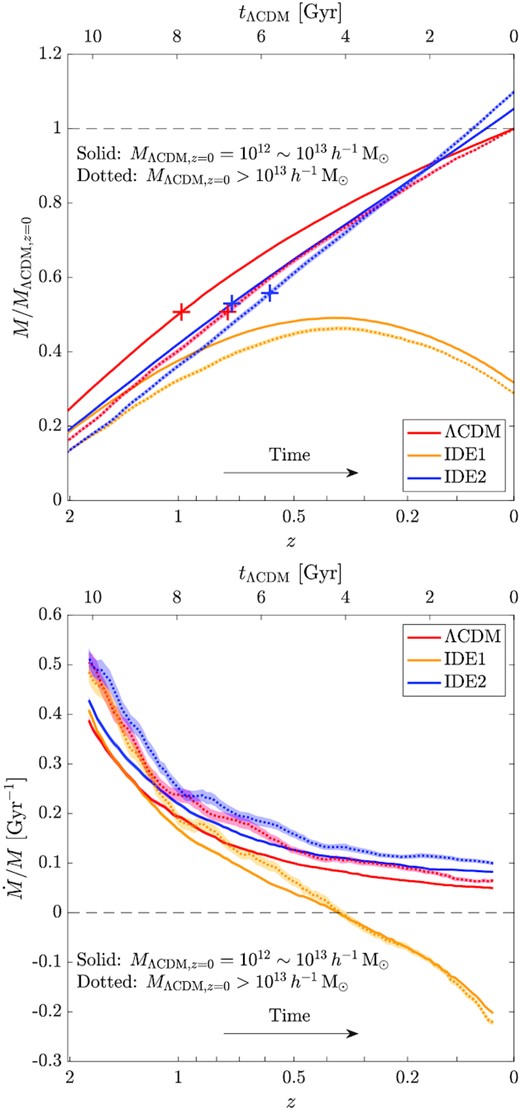
Top: average normalized mass growth history, M(z)/MΛCDM, z = 0, of haloes in ΛCDM (red), IDE1 (yellow), and IDE2 (blue) models. The solid and dotted lines show the low-mass and high-mass subsamples, respectively. The shaded region associated with each line represents the standard deviation of the means. The crosses mark the mean formation times. Bottom: similar to the top panel but for the average relative mass growth rate, |$\dot {M}/M$|.
In IDE1, the halo growth history is significantly different from that of the other two models. At z ∼ 2, being similar to the IDE2 haloes, the IDE1 haloes are less massive and grow slower comparing to the ΛCDM haloes. At z ∼ 1, their growth becomes even slower and the halo masses are considerably lower than their counterparts of both ΛCDM and IDE2. After z ∼ 0.4, the masses of IDE1 haloes even turn around and start to decrease. Because of this unique evolution history, the aforementioned formation time is ill-defined in the IDE1 model, and we thus do not compute the mean formation time for this model.
At z = 0, in comparison to the ΛCDM counterparts, IDE1 haloes end with a mass ratio of ∼0.3 while IDE2 haloes of ∼1.1. The mass difference between the ΛCDM model and the two IDE models is somewhat larger for the high-mass subsample than that of the low-mass subsample. This hints us that high-mass haloes might help to put tighter constraints on IDE models.
For ΛCDM, the |$\dot {M}/M$| decreases with cosmic time, reflecting that the growth of haloes slows down. For the high-mass part, |$\dot {M}/M$| is systematically higher than that of the low-mass subsample. This is related to the fact that high-mass haloes form later and their progenitors are typically in denser environments than the low-mass haloes.
Similar |$\dot {M}/M$| behaviours are seen in IDE2 except that the |$\dot {M}/M$| is higher than that of ΛCDM. At z ≳ 1, the |$\dot {M}$| are about the same for IDE2 and ΛCDM models as seen from the upper panel of Fig. 5. However, the halo mass is systematically lower, and thus the |$\dot {M}/M$| is higher for IDE2. At the late epoch, because of the interaction between the two dark components that converts dark energy to dark matter, the halo growth is faster in IDE2, leading to a higher |$\dot {M}/M$| and even the mass of IDE2 haloes is larger at redshift z ≲ 0.2 than that of ΛCDM.
On the other hand, for IDE1, at z ≳ 1, |$\dot {M}/M$| is about the same as that of ΛCDM for both high- and low-mass subsamples. This is because both |$\dot {M}$| and M are lower in IDE1. At z < 1, |$\dot {M}/M$| decreases much faster in IDE1 than the other two models and becomes negative at z ∼ 0.4. This is due to the interaction that dark matter decays into dark energy, which suppresses effectively the halo growth. At z ≲ 0.4, because of the decrease of the mass of dark matter particles, the gravitational potential of IDE1 haloes gets shallower, and some of the halo member particles become unbound. Furthermore, they cannot accrete more particles. As a result, IDE1 haloes are partially dissolved, and their mass decreases and thus the |$\dot {M}$| gets negative.
Our analyses here reveal clearly how the interaction between the two components affects the formation and evolution of dark matter haloes. It is noted that the model parameters we adopt for IDE1, IDE2, and ΛCDM are the ones that can fit the observational data of both CMB and cosmic expansion history. However, their non-linear structure formation is significantly different, showing solidly the importance of including non-linear structure probes to tighten the constraints on different cosmological models.
3.3 Halo density profile
In this subsection, we analyse the internal density profile of dark matter haloes at z = 0 for different models.
We measure the density profiles of the z = 0 host haloes with ≥1000 member particles in ALL sample and all the halo triplets in MATCH sample. For each halo, we first divide the halo particles into 20 elementary bins logarithmically distributed in radial distance ranging from |$0.01\, r_{200}$| to r200. From these, we construct 18 overlapped bins each comprising three elementary bins to enrich the particle numbers. As in the gadget code, the gravitational force only becomes exactly Newtonian beyond 2.8 times the softening length (i.e. ∼12 h−1 kpc in our simulations), we drop those inner bins whose radii are smaller than 12 h−1 kpc.
We find that the density profiles of the simulated dark matter haloes in considered IDE models can be well fitted by the NFW profile for the mass range of our samples. Fig. 6 presents a typical example of the density profiles for a halo triplet in MATCH sample, where the three matched haloes from IDE1, IDE2, and ΛCDM are the ones shown in the bottom row of Fig. 2. The points are measured from simulated haloes, and the lines are the fitted NFW profiles.
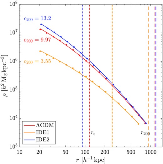
Density profiles of the ΛCDM halo (red) and its IDE1 (yellow) and IDE2 (blue) counterparts that are shown in the bottom row of Fig. 2. The data points are measured from simulations and the curve associated with each set of points is the corresponding NFW profile fitting. The best-fitting concentrations are given explicitly. The dotted and dashed vertical lines mark the corresponding rs and r200, respectively.
It is seen clearly that the IDE1 halo density profile markedly deviates from that of ΛCDM and IDE2 haloes. It is overall lower because of the lowest mass of the IDE1 halo. Furthermore, it is significantly flatter than that of the other two models. This is closely related to the interaction that leads to dark matter decaying into dark energy. Thus, the IDE1 halo cannot confine their member particles tightly. For IDE2, the profile is similar to that of ΛCDM but somewhat steeper due to the increase of the dark matter content converted from dark energy.
In Fig. 6, we also indicate the values of rs and r200 with vertical dotted and dashed lines, respectively, for the three haloes. The IDE1 halo has the largest rs and the smallest r200; therefore, its concentration is the smallest with c200 = 3.55. For IDE2 halo, its profile is the steepest with the smallest rs, and the value of r200 is about the same as that of the ΛCDM counterpart, resulting in the largest concentration of c200 = 13.2. For the ΛCDM halo, c200 = 9.97.
We emphasize that apart from the overall dimensional values of the halo density, its profile is independent of the dark matter particle mass in the haloes. Thus, by scaling the particle mass of IDE haloes to that of the ΛCDM, we can only shift up (IDE1) and down (IDE2) the density distributions, but their profiles, e.g. the values of the concentration parameters, remain to be unchanged. Therefore, the profile differences seen here indeed are the results of different halo formation histories among models.
In Fig. 7, we show the concentration–mass (c200–M200) relation at z = 0 for the ΛCDM, IDE1, and IDE2 models, where the solid lines show the median values and the shaded regions are the range from 25 to 75 percentiles. It is seen that for all the three models, the concentration decreases with the halo mass. This is consistent with the cold dark matter scenario where low-mass haloes form systematically earlier and thus more concentrate than the high-mass ones. We note that in Carlesi et al. (2014a), they studied dark matter halo properties for coupled quintessence models in which dark matter converts to dark energy. They also observe lower halo concentrations than that of the ΛCDM. Our IDE1 results are qualitatively consistent with theirs although quantitatively different because of the different models.
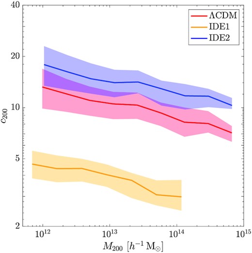
Concentration–mass relations of haloes in ΛCDM (red), IDE1 (yellow), and IDE2 (blue) models. The lines show the medians and the shaded region associated with each line represents the range from 25 to 75 percentile.
What is significant from Fig. 7 is that the c200–M200 curves of the three models are nearly parallel in the log–log space, implying a nearly constant ratio in c200 between IDE1 (IDE2) and ΛCDM independent of halo mass. We confirm this by analysing the MATCH sample. The results are shown in Fig. 8, where we contrast the concentration of each ΛCDM halo (horizontal axis) with that of its two IDE counterparts (vertical axis). Within each yellow (IDE1) or blue (IDE2) groups, the darker points are for more massive haloes. Clearly, the ratio of the halo concentrations between IDE and ΛCDM counterparts, |$\mathcal {R}=c_{200,\mathrm{IDE}}/c_{200,\Lambda \mathrm{CDM}}$|, is indeed approximately independent of the halo mass.
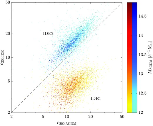
Contrast of halo concentrations between ΛCDM (horizontal axis) and IDE (vertical axis) counterparts. The yellow and blue groups show the results from IDE1 and IDE2, respectively. The colour depth indicates the corresponding halo mass in ΛCDM.
For IDE1 and IDE2, the ratio |$\mathcal {R}$| is very different. We expect it to depend on the interaction parameter, ξ2. Considering a simple Taylor expansion in |$\ln \mathcal {R}$| to the linear order, given |$\ln \mathcal {R}=0$| at ξ2 = 0, we have |$\ln \mathcal {R}=\alpha \xi _{2}$|. We fit this relation using the halo triplets in our MATCH sample. For enriching the data points, we further employ the IDE1′ and IDE2′ ones from the IDE1′-ΛCDM-IDE2′ triple-matched halo sample. The fitting is illustrated in Fig. 9, where we plot along the left and right vertical axes the distributions of |$\ln \mathcal {R}$| for IDE1 and IDE2 counterparts respectively, which can be well fitted by normal distributions. Similar distributions are seen for IDE1′ and IDE2′, which are not shown here. The red line is the fitting result with α = 8.04 ± 0.03, showing a positive correlation between |$\ln \mathcal {R}$| and ξ2. We see that |$\ln \mathcal {R}$| is very sensitive to the interaction parameter ξ2; thus, it can act as a powerful probe to constrain IDE models by measuring dark matter halo profiles accurately. This again demonstrates the importance of non-linear structures in differentiating different cosmological models.
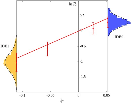
Correlation between the IDE-ΛCDM ratio of halo concentrations, |$\mathcal {R}=c_{200,\mathrm{IDE}}/c_{200,\Lambda \mathrm{CDM}}$|, and the interaction parameter, ξ2. The red line shows the fitting model, |$\ln \mathcal {R}=\alpha \xi _{2}$|, where α = 8.04 ± 0.03. The four red data points with error bars show the means and 1σ errors of |$\ln \mathcal {R}$| from IDE1, IDE1′, IDE2′, and IDE2, respectively. The distributions of |$\ln \mathcal {R}$|, and the corresponding normal fittings, from the best-fitting IDE1 (yellow) and IDE2 (blue) are shown along the vertical axes.
3.4 Halo spin
The spin of dark matter haloes is an important physical quantity that can affect directly the galaxy formation therein (e.g. Mo, Mao & White 1998). Its origin is closely connected with the initial tidal torques (Peebles 1969; Doroshkevich 1970; White 1984) and the halo formation history, particularly the merging history (Maller, Dekel & Somerville 2002; Vitvitska et al. 2002; Peirani, Mohayaee & de Freitas Pacheco 2004; D’Onghia & Navarro 2007). Here, we analyse halo spins for the IDE models. As before, we focus on the best-fitting IDE1 and IDE2 models, and we note that the results from IDE1′ and IDE2′ are similar but with smaller differences from the ΛCDM model.
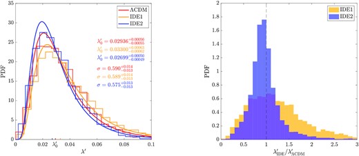
Left: distributions of halo spins in ΛCDM (red), IDE1 (yellow), and IDE2 (blue) models. The histograms are measured from simulations and the curve associated with each histogram is the corresponding lognormal fitting. The best-fitting |$\lambda _0^\prime$| and σ are given explicitly. Right: distributions of the IDE-ΛCDM ratios of λ′ from IDE1 (yellow) and IDE2 (blue). The vertical dashed line marks the ratio of 1.
In comparison to the ΛCDM haloes, the larger (smaller) λ′ of IDE1 (IDE2) counterparts indicates that the rotation component dominates more (less) for the total motions of member particles. This can be understood from two aspects. On the one hand, IDE1 (IDE2) haloes have smaller (larger) velocity dispersions than that of the ΛCDM counterparts given their shallower (deeper) potential wells as discussed in Section 3.3. On the other hand, as described in Section 2.2, there is an additional acceleration for the simulated particles in IDE models arising from the dark energy–dark matter interaction. It acts as accelerating (decelerating) the particles in IDE1 (IDE2) model, leading to an increase (decrease) of the specific angular momentum j. The combination of the two effects leads to the larger (smaller) values of λ′ for IDE1 (IDE2) haloes in comparison with that of ΛCDM.
3.5 Halo shape
Here, we further analyse the shape of dark matter haloes in different models. It is a non-trivial task to model the detailed shape of a realistic halo (see e.g. Jing & Suto 2002). In this study, following many literature on halo shapes, we model the dark matter halo as a 3D ellipsoid, which is characterized by its three orthogonal principal axes: a (major axis), b (intermediate axis), and c (minor axis) satisfying a ≥ b ≥ c.
We then calculate the axial ratios, b/a and c/a, for each halo in the MATCH sample. The probability distribution contours in b/a × c/a parameter space for the ΛCDM, IDE1, and IDE2 counterparts are shown in Fig. 11, where the top-right corner indicates spherical-like structures, and the bottom-left and -right are for prolate and oblate ones, respectively. We can see that for IDE1, the contours shift systematically toward the bottom and to the left, showing that IDE1 haloes tend to be more aspherical systematically than the ones in the other two models. For IDE2 haloes, their axial ratio distributions are about the same as that of ΛCDM.
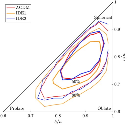
Distributions of halo shapes in ΛCDM (red), IDE1 (yellow), and IDE2 (blue) models in a b/a × c/a parameter space. The inner (thick) and outer (thin) lines show the |$50{{\ \rm per\ cent}}$| and |$80{{\ \rm per\ cent}}$| probability contours, respectively.
We also quantitatively confirm the above results by computing the IDE-ΛCDM ratios for b/a and c/a, as shown in Fig. 12. For IDE1, the medians are ∼0.98 and ∼0.96 for b/a and c/a ratios, respectively. For IDE2, both ratios are close to ∼1 based on our sample. For IDE1′ and IDE2′, the corresponding ratios are closer to 1. To be consistent with the results of halo spin, for IDE1 haloes, the additional acceleration of member particles arising from the dark energy–dark matter interaction prevents the halo relaxation and increases the halo anisotropy. Again, we observe a weak mass dependence from the filled and open histograms for low- and high-mass subsamples, respectively, in Fig. 12. The high-mass subsample of IDE1 shows a slightly larger deviation from that of the ΛCDM than the low-mass subsample.
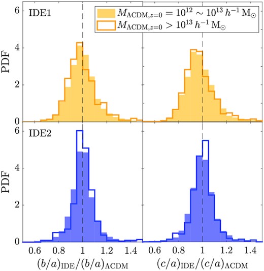
Distributions of the IDE-ΛCDM ratios of b/a (left column) and c/a (right column) from IDE1 (top row) and IDE2 (bottom row), respectively. The filled and open histograms show the low-mass and high-mass subsamples, respectively. The vertical dashed lines mark the ratio of 1.
4 CONCLUSIONS
Based on a set of self-consistent IDE and ΛCDM N-body simulations, we systematically analyse the formation history of dark matter haloes and their properties in IDE models and compare them with the ΛCDM counterparts. We aim to understand how the interaction between the two dark components in the Universe affects the non-linear cosmic structure formation and thus to find sensitive probes in constraining different cosmological models.
We investigate four IDE models, IDE1, IDE1′, IDE2, and IDE2′. All models have the dark energy–dark matter interactions proportional to the density of dark energy, but the signs of the interaction parameter ξ2 are different. For IDE1 and IDE1′, dark matter decays into dark energy while the opposite for IDE2 and IDE2′. The IDE1 and IDE2 employ the best-fitting parameters from previous constraints, and the ones marked with prime symbol employ the parameters of midpoint values between the ΛCDM and corresponding best-fitting models.
We summarize our main results from IDE1, IDE2, and their comparisons with ΛCDM as follows. The IDE1′ and IDE2′ behave similarly to the IDE1 and IDE2, respectively, but with smaller differences from ΛCDM.
The interaction of dark energy and dark matter affects the halo mass function significantly. In particular, for IDE1 in which dark matter decays into dark energy, the structure formation is slowed down, and the halo mass function is markedly lower than that of ΛCDM at low redshift. On the contrary, we observe a faster increase of the halo mass function from high to low redshift in IDE2 model where dark energy transfers to dark matter. The sensitive dependence of the halo mass function on the dark energy–dark matter interaction provides a powerful non-linear probe in constraining IDE models.
The halo formation history shows distinctly different behaviours in IDE models in comparison with ΛCDM model. The IDE2 haloes have larger mass growth rates |$\dot {M}$| and also the relative mass growth rates |$\dot {M}/M$| at low redshift. At z = 0, the mass ratio of haloes in IDE2 to their ΛCDM counterparts is ∼1.1. For IDE1 haloes, their growth is greatly suppressed at z ≲ 1 and even turns to be negative at z ≲ 0.4. As a result, at z = 0, the mass of IDE1 haloes is only about 0.3 times that of the ΛCDM counterparts. The mass contrast between IDE models and ΛCDM model shows a weak mass dependence with the high-mass subsample having a larger mass difference than the low-mass ones.
For the internal density profile of dark matter haloes, they all can be well fitted by the NFW functional form for both IDE and ΛCDM models. However, the characteristic halo parameters are very different for different models. Comparing to the ΛCDM counterparts, the IDE1 haloes have lower concentrations and internal potentials, and the IDE2 haloes show the opposite. Notably, we find that the IDE-ΛCDM ratio of halo concentrations, |$\mathcal {R}=c_{200,\mathrm{IDE}}/c_{200,\Lambda \mathrm{CDM}}$|, is nearly independent of halo mass. By fitting a simple linear model in |$\ln \mathcal {R}$|, i.e. |$\ln \mathcal {R}=\alpha \xi _2$|, we obtain α = 8.04 ± 0.03. This high value of α reflects a sensitive dependence of the halo internal density profile on the interaction parameter, offering an important means to constrain IDE models.
We also analyse the halo spin and shape for different models by measuring the specific spin parameter λ′, the axial ratios b/a and c/a, and the triaxiality parameter T. To compare with the ΛCDM counterparts, we find that IDE1 haloes have systematically larger λ′, smaller b/a and c/a, which indicate the structures of IDE1 haloes are more anisotropic, and dominated more by the overall rotations. IDE2 haloes have smaller λ′ than the ΛCDM counterparts, but the shape parameters are about the same. For all models, their haloes are primarily triaxial, and the T parameters for the haloes in ΛCDM and IDE models are about the same.
Our results quantitatively show the impacts of the interaction between dark energy and dark matter on non-linear structure formation. As the observed halo mass function and c200–M200 relation are largely consistent with the predictions from ΛCDM simulations (Tinker et al. 2008; Du et al. 2015; Xu et al. 2021), we can safely rule out the considered best-fitting parameter set of IDE1 although which can fit CMB and cosmic expansion history data well. This clearly shows the indispensable role of non-linear probes in cosmological studies. The approximately constant ratio of the |$\mathcal {R}=c_{200,\mathrm{IDE}}/c_{200,\Lambda \mathrm{CDM}}$| and its dependence on the interaction parameter promise a sensitive means to constrain IDE model parameters by measuring dark matter halo density profiles. The quantitative constraints based on our results and together with the observational data will be carried out in our future work.
In addition to the simulations of the five models presented in previous sections, we also run and analyse two toy IDE models with their cosmological parameters being the same as that of the ΛCDM model except ξ2 = −0.05 and wd = −0.999 for the IDE1-toy model and ξ2 = 0.05 and wd = −1.001 for the IDE2-toy model. Because of the matter density being normalized to the present observed value, the IDE1-toy model/IDE2-toy model has higher/lower Ωm(z) than that of ΛCDM, in contrast to the IDE models considered in the main text. By analysing the toy models, we find that while the quantitative results do depend on the cosmological parameter settings, qualitatively, all the IDE1-like models with dark matter transferring to dark energy show similar behaviours in slowing down the structure formation. On the other hand, for the IDE2-like models with dark energy converting to dark matter, the structure formation is getting strengthened towards the present time.
Limited by simulation resolutions, our investigations here focus mainly on host haloes with mass in ΛCDM model above 1012 h−1 M⊙. To further extend to smaller haloes, simulations of higher resolutions are needed. We also note that our simulations are dark matter only without including baryons. Although we do not expect qualitative changes about our conclusions regarding IDE1 and IDE2 in comparison with that of ΛCDM, detailed studies involving baryon physics are desirable in order to better confront with observations above and below galactic scales.
ACKNOWLEDGEMENTS
This work was inspired by the discussions during the second HOUYI Workshop for Non-standard Cosmological Models in Kunming, China, 2019. The calculations of this study were partly done on the Yunnan University Astronomy Supercomputer. YL acknowledges the supports from the Research |$\&$| Innovation Project for Postgraduates of Yunnan University (no. 2019z060) and from NSFC of China (no. 11973036). SHL acknowledges the support by the European Research Council via ERC Consolidator Grant KETJU (no. 818930). ZHF and XKL are supported by NSFC of China under grant no. 11933002 and no. U1931210, and a grant from the CAS Interdisciplinary Innovation Team. XKL also acknowledges the supports from NSFC of China under grant no. 11803028 and no. 12173033, YNU grant no. C176220100008, and the research grants from the China Manned Space Project with no. CMS-CSST-2021-B01. ZHF also acknowledges the supports from NSFC of China under no. 11653001, and the research grants from the China Manned Space Project with no. CMS-CSST-2021-A01. JJZ was supported by IBS under the project code, IBS-R018-D1, and the research grants from the China Manned Space Project with no. CMS-CSST-2021-A03. RA acknowledges the support from National Science Foundation under grant no. PHY-2013951 at USC.
DATA AVAILABILITY
The simulation data used in this article will be shared on reasonable request to the authors.
