


ABSTRACT
Gamma-ray bursts (GRBs) are ultra-relativistic collimated outflows, which emit synchrotron radiation throughout the entire electromagnetic spectrum when they interact with their environment. This afterglow emission enables us to probe the dynamics of relativistic blast waves, the microphysics of shock acceleration, and environments of GRBs. We perform Bayesian inference on a sample of GRB afterglow data sets consisting of 22 long GRBs and 4 short GRBs, using the afterglow model scalefit, which is based on 2D relativistic hydrodynamic simulations. We make use of Gaussian processes to account for systematic deviations in the data sets, which allows us to obtain robust estimates for the model parameters. We present the inferred parameters for the sample of GRBs and make comparisons between short and long GRBs in constant-density and stellar-wind-like environments. We find that in almost all respects such as energy and opening angle, short, and long GRBs are statistically the same. Short GRBs however have a markedly lower prompt gamma-ray emission efficiency than long GRBs. We also find that for long GRBs in ISM (interstellar medium)-like ambient media there is a significant anticorrelation between the fraction of thermal energy in the magnetic fields, ϵB, and the beaming corrected kinetic energy. Furthermore, we find no evidence that the mass-loss rates of the progenitor stars are lower than those of typical Wolf–Rayet stars.
1 INTRODUCTION
Gamma-ray bursts (GRBs) are the most powerful explosions in the Universe. They are ultra-relativistic collimated outflows, which are powered by a compact central object. GRBs are initially observed as brief flashes of gamma-rays lasting about 0.1–1000 s. These initial brief flashes of high-energy radiation are called the prompt emission of the GRB. The exact emission mechanism of the prompt emission remains elusive, despite decades of dedicated research. GRBs are phenomenologically categorized as short and long GRBs depending on the observed duration of the prompt emission phase (Kouveliotou et al. 1993). Short GRBs have been associated with compact object mergers where at least one of the objects is a neutron star (Lattimer & Schramm 1976; Eichler et al. 1989), whereas long GRBs are thought to be results of core-collapse supernovae of massive stars (Woosley 1993).
As the ejected ultra-relativistic outflow from a GRB starts to interact with the circumburst medium (CBM), a pair of shocks are generated, one of which propagates into the ejecta (reverse shock) and the other propagates into the CBM (forward shock). In these shocks, tangled magnetic fields are amplified and charged particles are accelerated, which results in long-lasting synchrotron emission spanning the whole electromagnetic spectrum (Rees & Mészáros 1992). This broad-band synchrotron emission is observable for several months, even years in some cases, and is called the afterglow emission of the GRB. The afterglow emission provides crucial insights on the energetics and environments of GRBs, the dynamics of relativistic blast waves, and the microphysics of particle acceleration in shocks (Wijers, Rees & Mészáros 1997; Sari, Piran & Narayan 1998; Wijers & Galama 1999; Panaitescu & Kumar 2002; Yost et al. 2003).
Thanks to missions like the Neil Gehrels Swift Observatory (Gehrels et al. 2004) and Fermi Gamma-ray Space Telescope (Atwood et al. 2009), the number of detected/localized GRBs has increased and allowed for rapid, ground/space based, broad-band follow-up observations of the afterglow emission. Moreover, the start of the multimessenger era has supplemented our understanding of the physics of GRBs (Abbott et al. 2017; MAGIC Collaboration et al. 2019). Besides advances in observational instruments, developments in numerical hydrodynamics and radiative transfer have enabled us to build models with increasing complexity and accuracy (e.g. De Colle et al. 2012; van Eerten, van der Horst & MacFadyen 2012; van Eerten & MacFadyen 2013; Ryan et al. 2015; Duffell & Laskar 2018; Wu & MacFadyen 2018; Jacovich, Beniamini & van der Horst 2021). Moreover, advances in statistical methods allow us to perform robust Bayesian inference and obtain reliable parameter estimates (Aksulu et al. 2020). Due to all these developments, we can now model a sample of GRB afterglow data sets, consistently, and investigate the distribution of physical parameters in the GRB population.
Previously, Panaitescu & Kumar (2002) and Yost et al. (2003) have performed broad-band afterglow modelling, and inferred burst parameters for a sample of long GRBs. Furthermore, Fong et al. (2015) have gathered data for a large number of short GRBs, and inferred their burst parameters based on their afterglow emission. These studies utilized semi-analytic models to reproduce the observed broad-band emission; in this study, we make use of a model based on 2D relativistic hydrodynamic (RHD) simulations. This allows us to capture the dynamics of these energetic events in a more realistic fashion.
In Aksulu et al. (2020) (A20, from now on), we introduced a new method for Bayesian parameter estimation, where we make use of Gaussian processes (GPs) in order to take into account some systematic effects in the data set and physics not included in the model. We showed in A20 that this approach allows us to obtain more robust parameter estimates, whereas the more conventional method of sampling the χ2 likelihood leads to underestimated uncertainties on the parameters, especially in the presence of systematics. We make use of a modified version of the GP model described in A20, in order to model a sample of 26 GRB afterglow data sets. In Section 2, we describe the GRB sample, model, inference approach, and details of the regression process. In Section 3, we present our results and the inferred physical parameters of the sample. Finally, we discuss our findings in Section 4 and conclude in Section 5. Throughout this work, we assume the cosmology as described in Planck Collaboration XIII et al. (2016).
2 METHOD
2.1 Sample
Our GRB afterglow sample consists of 26 GRBs with well-sampled, broad-band data sets. We relied only on peer-reviewed, published data sets, and converted the reported measurements to mJy units. The main selection criterion for the sample of GRBs has been the availability of broadband afterglow data. Twenty-two out of the 26 GRBs are long GRBs detected between 1997 and 2014, with published broad-band data sets; the time period is set to get a large enough sample. For short GRBs, we found only four with detections in radio, optical and X-ray bands up to the present. We omitted GRBs with non-canonical features in their light curves and include the five GRBs modelled in A20. When possible, we neglect epochs and/or bands for which there is evidence that the emission is dominated by processes that are not included in our model (e.g. early time optical and radio emission from GRB 130427A, which is dominated by reverse shock emission). This does not, of course, in any way represent a well-defined complete sample. We drew the boundary for having enough data somewhat subjectively, and similarly selected data sections in the early light curves suspected of unmodelled physics by eye.
We corrected the observed flux values for Galactic dust extinction using the extinction curve given by Pei (1992). We subtract any persistent emission originating from the host galaxy when possible. We do not correct the data for the dust extinction due to the host galaxy; instead we leave the rest-frame AV value for the host galaxy as a free parameter (see Section 2.3). We present the GRB sample in Table 1.
The GRB sample for this study. The measured redshift (z) and isotropic equivalent prompt energetics (Eγ, iso) are presented.
| Burst name | z | Eγ, iso/1052 (erg) | |
|---|---|---|---|
| Short GRBs | 051221A | 0.5465 | 0.15 |
| 130603B | 0.3564 | 0.21 | |
| 140903A | 0.351 | 0.006 ± 0.0003 | |
| 200522A | 0.5536 | 0.0084 ± 0.0011 | |
| Long GRBs | 970508 | 0.835 | 0.61 ± 0.13 |
| 980703 | 0.966 | 6.9 ± 0.8 | |
| 990510 | 1.619 | 17.8 ± 2.6 | |
| 991208 | 0.706 | 22.3 ± 0.8 | |
| 991216 | 1.02 | 67.5 ± 8.1 | |
| 000301C | 2.04 | 4.6 | |
| 000418 | 1.118 | 9.1 ± 1.7 | |
| 000926 | 2.066 | 27. ± 5.8 | |
| 010222 | 1.477 | 81. ± 1. | |
| 030329 | 0.1685 | 1.66 ± 0.2 | |
| 050820A | 2.615 | 97.5 ± 7.7 | |
| 050904 | 6.29 | 124. ± 7.7 | |
| 060418 | 1.49 | 12.8 ± 1 | |
| 090328 | 0.7357 | 13. ± 3 | |
| 090423 | 8.26 | 9.5 ± 2 | |
| 090902B | 1.8229 | 440 ± 30 | |
| 090926A | 2.1062 | 200 ± 5 | |
| 120521C | 6.0 | 8.25 ± 2 | |
| 130427A | 0.3399 | 81 | |
| 130702A | 0.145 | 0.064 ± 0.01 | |
| 130907A | 1.238 | 330. ± 10. | |
| 140304A | 5.283 | 12.24 ± 1.4 |
2.2 Gaussian process framework
GPs are stochastic processes that can be used for regression and classification problems for which the underlying physical model is unknown (e.g. Rasmussen & Williams 2006). Following A20 (also see Gibson et al. 2012), we make use of GPs to take into account any systematic deviations from the afterglow model. In this section, we highlight some improvements on the GP model introduced in A20. For clarity we use the same notation as in A20. Vectors and matrices are represented by bold symbols.
2.3 Model
The initial Lorentz factor of the blast wave is assumed to be uniform within the opening angle of the jet, i.e. a top hat jet model. We assume that charged particles are accelerated in the forward shock and emit synchrotron emission (Sari et al. 1998; Wijers & Galama 1999; Granot & Sari 2002). In this work, we do not take into account emission originating from the reverse shock and thus confine ourselves to fitting the later parts of the afterglow when the reverse shock has passed through the ejecta and the deceleration phase is over; in this limit, the value of the initial Lorentz factor of the jet is no longer important and need not (indeed, cannot) be fit. For the ‘microphysical’ parameters, which describe the spectrum and energy content of the electrons behind the blast wave and the magnetic field in which they move, we use the customary notation: p is the power-law index of the energy distribution of the relativistic electrons, and ϵe and ϵB are the fractions of post-shock energy density in relativistic electrons and magnetic field, respectively. Only a fraction of all electrons, ξN, may be accelerated. When p ≃ 2, the total energy in electrons and the value of p become very correlated in the fit, because the blast-wave emission depends on the combination |$\bar {\epsilon }_e \equiv \frac{p - 2}{p - 1}\epsilon _e$|. Therefore, we fit for that quantity and disentangle p and ϵe later where possible. Similarly, the fraction of accelerated electrons, ξN, is degenerate with respect to |$(E_{K,\mathrm{iso}}, n_\mathrm{ref}, \epsilon _B, \bar {\epsilon }_e)$|, where (EK,iso, nref) are proportional to 1/ξN, and |$(\epsilon _B, \bar{\epsilon }_e)$| are proportional to ξN (Eichler & Waxman 2005). Because of this degeneracy, we cannot determine ξN independently from afterglow light curves and fix it to the canonical value of 1 (for ease of comparison with previous studies).
We make use of the numerical model scalefit (Ryan et al. in preparation; Aksulu et al. 2020; Ryan et al. 2015). scalefit uses pre-calculated tables of spectral features (spectral breaks, peak spectral flux) for a range of different time epochs, opening angles, and observing angles. These tables are generated separately for ISM and wind-like circumburst density profiles using boxfit (van Eerten et al. 2012). boxfit is a numerical code which is able to output flux values for given observer time, frequency, and GRB parameters. The main advantage of boxfit is that the dynamics rely on pre-calculated RHD simulations. However, since boxfit solves the radiative transfer equations during runtime, it is computationally expensive. Therefore, it is not practical to use boxfit when performing Bayesian inference. Moreover, boxfit does not take into account the effects of synchrotron cooling on the self-absorption break. This may lead to incorrect spectra in certain regimes. scalefit, on the other hand, makes use of pre-calculated spectral features, obtained from boxfit in a valid regime, and utilizes scaling rules (van Eerten & MacFadyen 2012) to calculate the spectra for various regimes (i.e. different orderings of the break frequencies). scalefit is valid for all spectral regimes, unlike boxfit, and is computationally inexpensive in comparison (Ryan et al. in preparation). However, scalefit makes assumptions about the sharpness of the spectra around break frequencies, whereas boxfit generates smooth spectra in a self-consistent way.
Additionally, we account for dust extinction due to the host galaxy when calculating the observed flux. For the majority of GRBs in our sample, we adopt the Small Magellanic Cloud extinction curve given by Pei (1992). However, for GRBs 000418 (Gorosabel et al. 2003), 010222 (Frail et al. 2002), and 090328 (McBreen et al. 2010), we assume a Starburst type extinction curve (Calzetti et al. 2000). We include the dust extinction due to the host galaxy as a free parameter.
2.4 Regression
In order to obtain posterior distributions for the hyperparameters and model parameters, we make use of nested sampling (Skilling 2004). Incorporating nested sampling allows us to calculate the evidence with an associated numerical uncertainty, while producing posterior samples as a by-product. Inferring the Bayesian evidence is instrumental in this study, because it gives us a measure to determine which model explains the data best: a blast wave moving into a homogeneous (k = 0) or wind-like (k = 2) circumburst medium (see Section 2.3).
Following A20, we utilize pymultinest (Buchner et al. 2014), which is a python package based on the MultiNest nested sampling algorithm (Feroz, Hobson & Bridges 2009). For all the presented results, pymultinest is used in the importance sampling mode (Feroz et al. 2019) with mode separation disabled. We use 400 initial live points and use an evidence tolerance of 0.5 as our convergence criterion.
We assume wide priors for a and σh, however, the length-scale hyperparameters (i.e. l1 and l2) are capped at 1 (see Table 2), since we do not expect any systematics to be correlated over orders of magnitude (the GP model operates in the log-space). This is important, we found, because if one allows long correlation length-scales, the GP can take up features like constant offsets between model and data, or slope differences, which the model should really be capable of fitting. We intend the Gaussian process mostly to take up issues like calibration differences between instruments leading to extra ‘noise’ within a band, and physical effects that are shorter in time and frequency scale than is included in the model, such as radio scintillation, minor flares, etc.
Assumed priors for the GP hyperparameters.
| Parameter range | Prior distribution |
|---|---|
| 10−10 < a < 1010 | log-uniform |
| 10−6 < l1 < 1 | log-uniform |
| 10−6 < l2 < 1 | log-uniform |
| 10−3 < σh < 103 | log-uniform |
| Parameter range | Prior distribution |
|---|---|
| 10−10 < a < 1010 | log-uniform |
| 10−6 < l1 < 1 | log-uniform |
| 10−6 < l2 < 1 | log-uniform |
| 10−3 < σh < 103 | log-uniform |
For all the model parameters, we assume uninformative prior distributions, which can be seen in Table 3.
Assumed priors for the physical parameters.
| Parameter range | Prior distribution |
|---|---|
| 0.01 < θ0 < 1.6 | Log-uniform |
| 1050 < EK,iso < 1056 | Log-uniform |
| 10−3 < nref < 1000 | Log-uniform |
| 0 < θobs/θ0 < 2 | Uniform |
| 1.0 < p < 3.0 | Uniform |
| 10−10 < ϵB < 1.0 | Log-uniform |
| |$10^{-10}\lt \bar{\epsilon _e}\lt 10$| | Log-uniform |
| 0 < AV < 10 | Uniform |
Note that we do not take into account any reported upper limits on the afterglow flux when inferring parameters, since upper limit reports typically do not contain enough information to include them in the fitting in a statistically sound way.
3 RESULTS
In this section, we present the modelling results for our sample of 26 GRB afterglow data sets (see Table 1). We will not discuss individual GRBs in detail, since the objective of our work is to examine the properties of a population of GRB afterglow sources and systematics of how the properties are distributed and may differ between subclasses. In so doing, we will examine correlations between each pair of fit parameters and distributions of fit parameters between each of a few subclasses. All in all, we make about 50 such comparisons, and therefore we have a fair chance of finding differences or correlations at the few per cent probability level by statistical coincidence. To account for this, we will only regard correlations or differences in distributions as firmly significant when the null hypothesis of no correlation or no difference can be excluded at the single-trial p-value of 3 × 10⁻⁴ or better, and tentative below p = 1 × 10⁻³. Of course, since we do not have a statistically complete sample, we should not only examine the statistical significances but also the possible effect of biases.
We find that in all cases the best-fitting values of the parameters and their 68 per cent credible intervals remain naturally contained within the range set by the priors, and in most cases, this is still true for the 95 per cent credible interval. We also find that in individual cases there can be strong correlations between parameter errors due to degeneracies in a specific fit, but we did not find any that were common enough to induce correlations between parameters in the overall population. We also find that for all physical parameters the range of best-fit values is significantly larger than the error regions of the better constrained afterglows. This implies that there are no physical parameters, specifically also not the shock microphysics parameters or the beaming-corrected energy, that prefer a universal value. This is in agreement with previous studies (e.g. Starling et al. 2008; Curran et al. 2009; Ryan et al. 2015), but now for a large and uniformly analysed sample of GRBs.
For our further description of the results, we focus on groups of physical parameters, from the outside in. We begin with the ambient density, since this is the first distinction we make, and it is made in a way somewhat different to the others, by comparing two different model fits. All others are simply free parameters fit within a certain constrained but continuous range. Of these, we first discuss the energy and geometrical parameters (opening angle and viewing angle), and after that the shock microphysics parameters.
3.1 GRB environment and ambient medium
We do not assume a priori which model, homogeneous or wind-like environment, should be chosen for a given data set. Instead, we model every data set both for homogeneous and wind-like environment models, and choose which one explains the data best. Model selection is performed by comparing the evidence values from both fits. We present the log-evidence values, along with the corresponding Bayes factors, for each modelling effort in Table 4. The Bayes factor, i.e. ratio of the evidence values, allows us to quantify the likelihood of the preferred model over the alternative model. A Bayes factor larger than 20 (e.g. Kass & Raftery 1995) suggests a strong preference for the selected model. Fifteen out 26 GRBs in our sample, all long, have a Bayes factor larger than 20, and 8 out of these GRBs show evidence for a constant density environment. Thus, if we only consider the GRBs with a strong preference, there is an approximately even split between homogeneous and wind-like environments. Starling et al. (2008) have analysed a sample of 10 GRBs and commented on their CBM density profile. They also find that both ISM-like and wind-like environments are required to explain the observed light curves for their sample of GRBs. Curran et al. (2009) have analysed the optical and X-ray light curves of 10 GRB afterglows, and arrived at the same conclusion. Schulze et al. (2011) have compiled a sample of 27 Swift detected GRBs (including one short GRB), and utilized the observed X-ray and optical afterglow emission to comment on the density profiles of their environments. They are able to determine that 18 GRBs in their sample are consistent with homogeneous environments, and 6 GRBs are consistent with wind-like environments. If we do not restrict ourselves to high Bayes factors, a slightly higher fraction of afterglows favours an ISM solution (16 out of 25, i.e. 64 per cent).
Model selection for the GRB sample. |$\mathcal {Z}$| represents the Bayesian evidence. Reported uncertainties represent 1–σ. We select the mode, either homogeneous (ISM) or wind-like environment, with higher inferred evidence values. The evidence values for the preferred model are written in bold numerals.
| Burst name | |$\ln \mathcal {Z}$| [ISM] | |$\ln \mathcal {Z}$| [Wind] | Bayes factor | |
|---|---|---|---|---|
| short GRBs | 051221A | |$\mathbf {-22.79 \pm 0.04}$| | −24.26 ± 0.12 | 4.33 |
| 130603B(a) | −21.45 ± 0.05 | −21.42 ± 0.03 | ∼1. | |
| 140903A | |$\mathbf {-24.97 \pm 0.05}$| | −25.73 ± 0.02 | 2.15 | |
| 200522A | |$\mathbf {-18.31 \pm 0.03}$| | −19.30 ± 0.02 | 2.68 | |
| long GRBs | 970508 | −99.21 ± 0.12 | |$\mathbf {-92.68 \pm 0.31}$| | >150 |
| 980703 | −86.74 ± 0.02 | |$\mathbf {-82.33 \pm 0.06}$| | 82.80 | |
| 990510 | |$\mathbf {279.21 \pm 0.02}$| | 278.45 ± 0.03 | 2.15 | |
| 991208 | |$\mathbf {-60.33 \pm 0.04}$| | −67.63 ± 0.10 | >150 | |
| 991216 | −5.37 ± 0.04 | |$\mathbf {-4.56 \pm 0.03}$| | 2.25 | |
| 000301C | |$\mathbf {37.45 \pm 0.05}$| | 25.30 ± 0.12 | >150 | |
| 000418 | −55.09 ± 0.04 | |$\mathbf {-49.81 \pm 0.05}$| | >150 | |
| 000926 | 28.31 ± 0.08 | |$\mathbf {34.48 \pm 0.04}$| | >150 | |
| 010222 | |$\mathbf {37.34 \pm 0.04}$| | 31.01 ± 0.02 | >150 | |
| 030329 | |$\mathbf {-29.23 \pm 0.01}$| | −59.81 ± 0.05 | >150 | |
| 050820A | −40.26 ± 0.74 | |$\mathbf {-33.88 \pm 0.05}$| | >150 | |
| 050904 | |$\mathbf {-31.20 \pm 0.03}$| | −33.30 ± 0.07 | 8.13 | |
| 060418 | |$\mathbf {-11.55 \pm 0.06}$| | −19.19 ± 0.02 | >150 | |
| 090328 | |$\mathbf {-50.14 \pm 0.03}$| | −51.69 ± 0.30 | 4.71 | |
| 090423 | |$\mathbf {-51.42 \pm 0.06}$| | −55.97 ± 0.10 | 94.59 | |
| 090902B | −49.39 ± 0.02 | |$\mathbf {-39.78 \pm 0.04}$| | >150 | |
| 090926A | |$\mathbf {-9.68 \pm 0.03}$| | −12.24 ± 0.02 | 12.98 | |
| 120521C | |$\mathbf {-54.96 \pm 0.06}$| | −55.50 ± 0.09 | 1.70 | |
| 130427A | 324.52 ± 0.08 | |$\mathbf {336.86 \pm 0.03}$| | >150 | |
| 130702A | |$\mathbf {19.45 \pm 0.18}$| | 8.55 ± 0.68 | >150 | |
| 130907A | |$\mathbf {-135.85 \pm 0.01}$| | −141.59 ± 0.02 | >150 | |
| 140304A | −60.46 ± 0.04 | |$\mathbf {-57.90 \pm 0.04}$| | 13.00 |
aFor this data set, both homogeneous and wind-like models result in similar evidence values. An ISM-type environment is preferred since this is a short GRB and no strong winds are expected due their progenitors.
For the short GRB sample the evidence values for both models are closer to each other. This is mainly due to the fact that short GRBs have fewer observations available, and therefore the data sets are less constraining; importantly, none of the short GRBs favour a wind environment, in agreement with the usual notion that they occur in less dense and near-uniform ISM. For short GRB 130603B, the evidence values for homogeneous and wind-like environments are consistent with each other considering the evidence uncertainty. Given that an ISM environment is a priori favoured, we chose that solution.
The wider environment of the GRB is also probed by the host extinction, AV. This is of course biased to somewhat low values by the fact that we want well-detected optical afterglows, and for short GRBs to somewhat higher values because we need them to lie in regions of not too low density to produce a detectable afterglow. We find that more than half the afterglows have a non-zero AV with better than 2σ significance, with no significant differences between short and long GRBs or wind and uniform ambient media.
Now that we have found the best ambient-density model for each afterglow, we will look at the other parameters, for which we take the values for the best-fitting ambient medium in each case. We present our modelling results for the GRB parameters (including the rest-frame host extinction values, AV) in Table 5. In Figs A1–A3, we present the posterior distribution for each parameter (in the form of a violin plot) together with their 68 per cent credible intervals. The complete set of light curves and posterior distributions are available as online supplementary material, including results for both homogeneous and wind-like environments for each GRB in our sample.
Inferred physical parameters for the GRB sample. The presented values correspond to the mode of the obtained posterior distribution. Reported uncertainties represent the 68 per cent credible interval. k represents the CBM density profile (see equation 4) and is either 0 for homogeneous or 2 for wind-like environments.
| Burst name | log10θ0 (rad) | log10EK,iso (erg) | log10nref | θobs/θ0 | p | log10ϵB | |$\log _{10}\bar{\epsilon }_e$| | AV | k | |
|---|---|---|---|---|---|---|---|---|---|---|
| Short GRBs | 051221A | |$-0.98^{+0.13}_{-0.17}$| | |$54.48^{+0.80}_{-1.69}$| | |$0.55^{+1.26}_{-1.80}$| | |$0.92^{+0.11}_{-0.29}$| | |$1.78^{+0.17}_{-0.10}$| | |$-2.40^{+0.91}_{-2.17}$| | |$-5.26^{+2.43}_{-1.25}$| | |$0.10^{+0.26}_{-0.10}$| | 0 |
| 130603B | |$-0.97^{+0.28}_{-0.54}$| | |$53.89^{+0.82}_{-1.17}$| | |$-1.14^{+0.59}_{-1.36}$| | |$0.83^{+0.13}_{-0.36}$| | |$2.67^{+0.25}_{-0.38}$| | |$-4.71^{+1.72}_{-3.85}$| | |$-0.98^{+0.51}_{-0.56}$| | |$0.74^{+0.44}_{-0.32}$| | 0 | |
| 140903A | |$-1.15^{+0.35}_{-0.22}$| | |$54.58^{+0.57}_{-1.20}$| | |$-1.97^{+1.17}_{-0.82}$| | |$0.41^{+0.26}_{-0.33}$| | |$2.36^{+0.17}_{-0.53}$| | |$-7.21^{+3.58}_{-1.82}$| | |$-1.07^{+0.63}_{-1.98}$| | |$0.22^{+0.32}_{-0.22}$| | 0 | |
| 200522A | |$-0.22^{+0.39}_{-0.31}$| | |$53.54^{+1.08}_{-0.78}$| | |$1.94^{+0.51}_{-1.48}$| | |$0.51^{+0.35}_{-0.20}$| | |$1.84^{+0.06}_{-0.06}$| | |$-7.75^{+1.89}_{-1.27}$| | |$-3.39^{+1.32}_{-1.33}$| | |$5.29^{+2.79}_{-3.33}$| | 0 | |
| Long GRBs | 970508 | |$0.06^{+0.03}_{-0.05}$| | |$53.20^{+0.22}_{-0.21}$| | |$2.18^{+0.11}_{-0.14}$| | |$1.08^{+0.04}_{-0.03}$| | |$2.57^{+0.05}_{-0.05}$| | |$-4.39^{+0.38}_{-0.27}$| | |$-0.49^{+0.05}_{-0.09}$| | |$0.13^{+0.07}_{-0.05}$| | 2 |
| 980703 | |$-0.34^{+0.26}_{-0.20}$| | |$52.28^{+0.36}_{-0.19}$| | |$0.50^{+0.25}_{-0.30}$| | |$0.89^{+0.16}_{-0.55}$| | |$2.07^{+0.05}_{-0.10}$| | |$-0.53^{+0.43}_{-0.57}$| | |$-1.89^{+0.20}_{-0.17}$| | |$1.01^{+0.16}_{-0.12}$| | 2 | |
| 990510 | |$-1.16^{+0.03}_{-0.05}$| | |$52.99^{+0.11}_{-0.08}$| | |$-0.95^{+0.15}_{-0.35}$| | |$0.31^{+0.13}_{-0.07}$| | |$1.93^{+0.06}_{-0.05}$| | |$-1.25^{+0.42}_{-0.45}$| | |$-1.54^{+0.09}_{-0.12}$| | |$0.01^{+0.02}_{-0.01}$| | 0 | |
| 991208 | |$-1.94^{+0.19}_{-0.06}$| | |$54.64^{+0.10}_{-0.41}$| | |$-0.60^{+0.19}_{-0.11}$| | |$1.05^{+0.41}_{-0.82}$| | |$1.61^{+0.08}_{-0.06}$| | |$-0.07^{+0.07}_{-0.16}$| | |$-1.33^{+0.12}_{-0.11}$| | |$0.44^{+0.09}_{-0.08}$| | 0 | |
| 991216 | |$-0.59^{+0.37}_{-0.25}$| | |$53.71^{+0.23}_{-0.44}$| | |$1.28^{+0.23}_{-0.52}$| | |$0.79^{+0.14}_{-0.41}$| | |$2.14^{+0.20}_{-0.08}$| | |$-3.61^{+0.54}_{-0.82}$| | |$-1.27^{+0.23}_{-0.23}$| | |$0.07^{+0.11}_{-0.06}$| | 2 | |
| 000301C | |$-0.69^{+0.03}_{-0.03}$| | |$52.42^{+0.16}_{-0.08}$| | |$0.33^{+0.47}_{-0.11}$| | |$0.07^{+0.04}_{-0.07}$| | |$1.88^{+0.10}_{-0.06}$| | |$-0.21^{+0.14}_{-0.78}$| | |$-1.52^{+0.19}_{-0.07}$| | |$0.03^{+0.08}_{-0.02}$| | 0 | |
| 000418 | |$-0.26^{+0.27}_{-0.29}$| | |$54.47^{+1.00}_{-0.82}$| | |$1.11^{+0.70}_{-1.12}$| | |$0.26^{+0.28}_{-0.20}$| | |$2.38^{+0.15}_{-0.18}$| | |$-1.91^{+0.52}_{-4.22}$| | |$-1.59^{+0.45}_{-0.50}$| | |$1.22^{+0.40}_{-0.29}$| | 2 | |
| 000926 | |$-0.24^{+0.31}_{-0.28}$| | |$55.13^{+0.63}_{-0.46}$| | |$1.99^{+0.79}_{-0.39}$| | |$0.34^{+0.20}_{-0.33}$| | |$2.96^{+0.04}_{-0.04}$| | |$-6.21^{+1.51}_{-1.08}$| | |$-0.95^{+0.34}_{-0.28}$| | |$0.20^{+0.05}_{-0.04}$| | 2 | |
| 010222 | |$-0.40^{+0.05}_{-0.22}$| | |$53.94^{+0.17}_{-0.15}$| | |$-2.32^{+0.19}_{-0.17}$| | |$0.13^{+0.29}_{-0.09}$| | |$2.62^{+0.03}_{-0.04}$| | |$-4.18^{+0.52}_{-0.31}$| | |$-0.47^{+0.06}_{-0.08}$| | |$0.54^{+0.05}_{-0.05}$| | 0 | |
| 030329 | |$0.20^{+0.01}_{-0.07}$| | |$53.04^{+0.10}_{-0.10}$| | |$2.59^{+0.20}_{-0.18}$| | |$0.73^{+0.05}_{-0.05}$| | |$2.62^{+0.02}_{-0.06}$| | |$-5.58^{+0.38}_{-0.33}$| | |$-0.76^{+0.08}_{-0.06}$| | |$0.01^{+0.02}_{-0.01}$| | 0 | |
| 050820A | |$-0.44^{+0.24}_{-0.21}$| | |$53.24^{+0.12}_{-0.11}$| | |$0.95^{+0.23}_{-0.16}$| | |$0.70^{+0.10}_{-0.39}$| | |$2.11^{+0.14}_{-0.07}$| | |$-1.95^{+0.19}_{-0.49}$| | |$-1.31^{+0.25}_{-0.18}$| | |$0.37^{+0.06}_{-0.08}$| | 2 | |
| 050904 | |$-1.02^{+0.12}_{-0.04}$| | |$53.31^{+0.28}_{-0.17}$| | |$1.05^{+0.25}_{-0.87}$| | |$0.54^{+0.21}_{-0.13}$| | |$2.11^{+0.08}_{-0.08}$| | |$-2.07^{+0.50}_{-0.46}$| | |$-1.54^{+0.13}_{-0.40}$| | |$0.07^{+0.05}_{-0.03}$| | 0 | |
| 060418 | |$-0.82^{+0.06}_{-0.07}$| | |$52.88^{+0.17}_{-0.14}$| | |$0.23^{+0.56}_{-0.36}$| | |$0.83^{+0.05}_{-0.06}$| | |$2.28^{+0.06}_{-0.04}$| | |$-2.81^{+0.32}_{-0.65}$| | |$-1.30^{+0.17}_{-0.13}$| | |$0.17^{+0.05}_{-0.05}$| | 0 | |
| 090328 | |$-0.68^{+0.20}_{-0.13}$| | |$53.17^{+0.51}_{-0.86}$| | |$1.66^{+0.70}_{-0.79}$| | |$0.94^{+0.23}_{-0.33}$| | |$2.28^{+0.10}_{-0.18}$| | |$-3.90^{+1.31}_{-0.89}$| | |$-1.39^{+0.48}_{-0.37}$| | |$0.07^{+0.11}_{-0.06}$| | 0 | |
| 090423 | |$-0.06^{+0.26}_{-0.10}$| | |$53.46^{+0.50}_{-0.48}$| | |$2.01^{+0.75}_{-0.62}$| | |$0.84^{+0.11}_{-0.46}$| | |$2.16^{+0.17}_{-0.24}$| | |$-4.81^{+1.48}_{-0.97}$| | |$-1.41^{+0.35}_{-0.56}$| | |$0.09^{+0.09}_{-0.07}$| | 0 | |
| 090902B | |$0.04^{+0.11}_{-0.34}$| | |$53.43^{+0.23}_{-0.37}$| | |$0.50^{+0.58}_{-0.31}$| | |$0.24^{+0.19}_{-0.22}$| | |$2.23^{+0.04}_{-0.09}$| | |$-3.15^{+0.70}_{-0.91}$| | |$-1.57^{+0.29}_{-0.23}$| | |$0.07^{+0.06}_{-0.06}$| | 2 | |
| 090926A | |$-0.81^{+0.08}_{-0.10}$| | |$53.09^{+1.17}_{-0.32}$| | |$0.19^{+2.07}_{-0.26}$| | |$0.78^{+0.25}_{-0.14}$| | |$2.24^{+0.08}_{-0.05}$| | |$-1.57^{+0.41}_{-2.14}$| | |$-0.93^{+0.28}_{-0.81}$| | |$0.09^{+0.01}_{-0.01}$| | 0 | |
| 120521C | |$-0.91^{+0.11}_{-0.11}$| | |$52.98^{+0.23}_{-0.16}$| | |$-0.47^{+0.41}_{-0.29}$| | |$0.50^{+0.20}_{-0.34}$| | |$2.88^{+0.12}_{-0.25}$| | |$-1.10^{+0.37}_{-0.51}$| | |$-0.84^{+0.16}_{-0.16}$| | |$0.78^{+0.09}_{-0.09}$| | 0 | |
| 130427A | |$-0.23^{+0.25}_{-0.15}$| | |$52.58^{+0.64}_{-0.17}$| | |$0.17^{+0.33}_{-0.53}$| | |$0.20^{+0.34}_{-0.20}$| | |$2.16^{+0.04}_{-0.05}$| | |$-2.31^{+0.62}_{-0.94}$| | |$-1.13^{+0.20}_{-0.25}$| | |$0.03^{+0.03}_{-0.03}$| | 2 | |
| 130702A | |$-0.71^{+0.12}_{-0.05}$| | |$53.07^{+0.90}_{-0.97}$| | |$-0.90^{+1.42}_{-0.45}$| | |$0.04^{+0.11}_{-0.04}$| | |$1.46^{+0.08}_{-0.04}$| | |$-0.71^{+0.63}_{-1.24}$| | |$-7.65^{+2.05}_{-1.89}$| | |$0.26^{+0.18}_{-0.12}$| | 0 | |
| 130907A | |$-1.38^{+0.17}_{-0.05}$| | |$53.02^{+0.34}_{-0.09}$| | |$-1.26^{+0.12}_{-0.11}$| | |$0.88^{+0.23}_{-0.21}$| | |$1.87^{+0.09}_{-0.09}$| | |$-0.04^{+0.04}_{-0.10}$| | |$-1.03^{+0.14}_{-0.18}$| | |$1.60^{+0.15}_{-0.16}$| | 0 | |
| 140304A | |$-1.30^{+0.23}_{-0.07}$| | |$54.46^{+0.28}_{-0.42}$| | |$1.96^{+0.57}_{-0.35}$| | |$1.19^{+0.34}_{-0.13}$| | |$2.28^{+0.17}_{-0.25}$| | |$-3.73^{+0.76}_{-0.72}$| | |$-1.40^{+0.20}_{-0.33}$| | |$0.41^{+0.11}_{-0.08}$| | 2 |
3.2 Energy, opening angle, and viewing angle
In Figs 1 and 2, we present the parameter values for the GRBs associated with homogeneous and wind-like environments, respectively, in the form of a corner plot. These figures help us to identify any correlations between the burst parameters. The diagonal elements in each figure contain the parameter distributions for the single fit parameters, with different colours for the short (green), long-ISM (blue), and long-wind (red) GRBs.
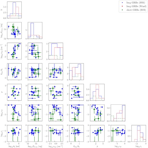
Corner plot for the inferred physical parameters of the GRBs associated with constant density environments. Blue circles and green squares represent the inferred parameter value of long GRBs and short GRBs, respectively. The error bars represent the 68 per cent credible limit.
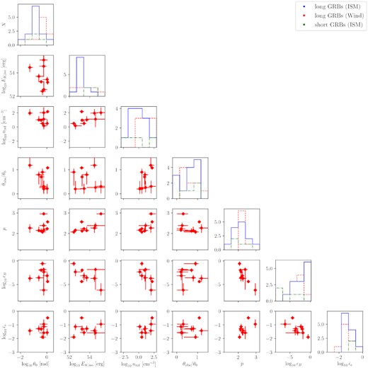
Corner plot for the inferred physical parameters of the GRBs associated with wind-like environments. The error bars represent the 68 per cent credible limit.
3.2.1 Opening angle
We do not find a notably different opening angle distribution for short and long GRBs. When a Kolmogorov–Smirnov (KS) test is performed on the inferred opening angle of ISM-like long GRBs and short GRBs, we find a p-value of 0.48 for the hypothesis that the two samples are drawn from the same distribution. A KS test checking the consistency of the θ0 distribution between ISM- and wind-like long GRBs yields we find p = 0.012. On its own that might be considered moderate evidence for a difference, but given the many trials (distribution comparisons) in this paper, it is not (see above).
3.2.2 Observer viewing angle
The distribution of the observer viewing angle, θobs, does not follow a simple form, since it is constrained to be within the jet opening angle (at least at early times), but that is different for each GRB as we have just seen. However, the fractional observer angle distribution, θobs/θ0, does have a simpler form under the top-hat jet assumption, because in that case every direction within the opening angle has the same properties and thus the same brightness at early times: its probability density is linear for θ0 ≪ π/2 and a sine function for θ0 = π/2. We show the distribution for the full sample in Fig. 3, with the two limiting theoretical cases. The observed distribution extends a bit beyond 1, but no values are significantly larger than 1. Even so, KS-comparison with the theoretical distributions gives p = 0.17 for accepting the null hypothesis of equality. We conclude that the data are consistent with the top-hat jet hypothesis and do not strongly indicate a structured, more centrally concentrated jet (which would closely resemble a top-hat jet for observers close to the jet axis in any case, e.g. Dalal, Griest & Pruet 2002; Rossi, Lazzati & Rees 2002; Granot & Kumar 2003; Kumar & Granot 2003; Panaitescu & Kumar 2003; Salmonson 2003; Rossi et al. 2004; Ryan et al. 2020). Specifically, our viewing angle has to be within the opening angle of the gamma-ray emission, which typically comes from material with Γ > 100. If the early afterglow emission, of which we derive the opening angle in our fits, had a significantly greater opening angle, then we would find the distribution of θobs/θ0 biased towards small values. Since the afterglow represents all the material with Γ ≳ 10, this means our result argues against jet structures in which the material with initial Lorentz factors above 10 has a significantly wider opening angle than the material with initial Lorentz factors above 100. This may argue against, or at least significantly constrain so-called jet-cocoon models of GRBs, in which a core jet with quite high initial Lorentz factors (Γ0 ≳ 100) is surrounded by an energetic cocoon with Lorentz factors of several tens (e.g. Ramirez-Ruiz, Celotti & Rees 2002; Peng, Königl & Granot 2005). The initial conditions of the simulations underlying our model are already outside the progenitor object. We do not think our afterglow selection has biased us against jet-cocoon cases: if the cocoon only decelerated after our afterglow data start, it would give rise to a late-injection or plateau phase in the afterglow (Granot & Kumar 2006; van Eerten 2014), and we have not excluded any afterglows for obvious signs thereof. If the cocoon decelerated before our afterglow data start, then the tendency to smaller observer angles because of the gamma-ray selection would remain, and we do not see this.
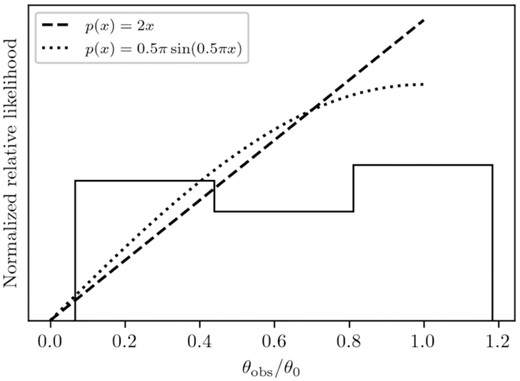
Histogram of the inferred θobs/θ0 for the GRB sample. The dotted line represents the analytically expected probability density function for large opening angles (θ0 = π/2 rad), whereas the dashed line represents the probability density function for small opening angles (θ0 ≪ π/2 rad).
The results on the GRB energy are more complex, and we defer them to the discussion section.
3.3 Shock physics parameters
For the shock physics parameters, we have to be a bit careful (see Section 2.3): in order to avoid too strong degeneracies for p ≃ 2, we fit for p and |$\bar {\epsilon }_e$|, and indeed we do find some cases of p < 2. The distribution of p, the power-law index of the shock-accelerated particles, can be seen in Fig. 4. We find that the p-values are consistent with being drawn from the same distribution for long GRBs and short GRBs. We find a mean value of 2.21 and standard deviation σp = 0.36 for the inferred p values. Curran et al. (2010) have analysed a large sample of Swift detected GRBs to determine the distribution of p. They utilized the reported spectral indices in X-rays to determine the p-values of their sample, using closure relations. They find that the distribution of p is consistent with a Gaussian distribution with μ = 2.36 and σ = 0.59; given the errors in both methods, we consider the two results to be consistent. We find three cases where p is significantly less than 2, and thus where a high-energy cut-off to the electron distribution is required to keep the total electron energy finite. In more than half the cases (15), p = 2 is included within the 95 per cent confidence region of the fit result, implying that indeed using |$\bar {\epsilon }_e$| is required to avoid problems in the fitting process.
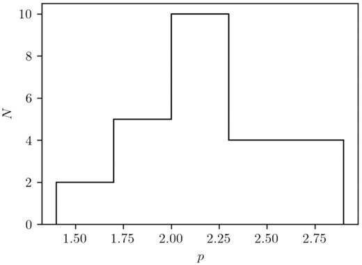
Histogram of the inferred p for the GRB sample.
While the short GRBs all have ϵB values on the low side, their small number and large error bars prevent us from drawing any strong conclusions in this respect: the KS test results in p = 0.10 for the short/long GRB distributions of magnetic-field energy fractions being the same, and similarly, we find no evidence for a difference between the long GRBs in ISM and wind environments. What is quite striking though is that ϵB ranges over 5–6 decades in value, a much greater range than ϵe.
Since ϵe is a physically more meaningful measure of the electron energy density, we derive it from the nominal fit values in case p > 2. The derived ϵe values can be seen in Table 6. In Fig. 5, we present the ϵe distribution of the GRB sample, only for GRBs with inferred mode value of p > 2. We find that ϵe is never very low and always above 0.1, with some values (uncomfortably?) close to 1. The values for the different subsamples are in good agreement (mean values are 0.34 for homogeneous environment and 0.28 for wind). Beniamini & van der Horst (2017) have demonstrated that it is possible to constrain ϵe by measuring the peak flux and peak time of the radio afterglow light curve. By applying this method to a sample of 36 long GRBs, they were able to put upper limits on the scatter of ϵe. They find that |$\sigma _{\log _{10}\epsilon _e} \lt 0.31$| for constant density environments and |$\sigma _{\log _{10}\epsilon _e} \lt 0.26$| for wind-like environments. We find that the standard deviation of ϵe for the long GRB sample is |$\sigma _{\log _{10}\epsilon _e} = 0.24$| for homogeneous environments and |$\sigma _{\log _{10}\epsilon _e} = 0.28$| for wind-like environments. Note that, although the standard deviations of the inferred ϵe distributions are consistent with Beniamini & van der Horst (2017), they find lower mean values of 0.15 and 0.13 for ISM-like and wind-like long GRBs, respectively.
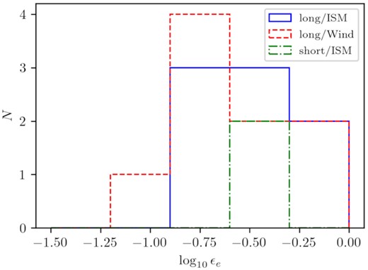
Histogram of the inferred ϵe for the GRB sample.
Derived parameters for the GRB sample. The presented values correspond to the mode of the obtained posterior distribution. Reported uncertainties represent the 68 per cent credible interval. We calculate ϵe values only for GRBs for which the inferred mode of p is larger than 2. Missing values are represented by -. k represents the CBM density profile (see equation 4) and is either 0 for homogeneous or 2 for wind-like environments.
| Burst name | log10ϵe | log10EK,true (erg) | log10Eγ,true (erg) | log10Etrue (erg) | log10ϵγ | k | |
|---|---|---|---|---|---|---|---|
| Short GRBs | 051221A | – | |$51.33^{+1.45}_{-1.00}$| | |$48.93^{+0.28}_{-0.35}$| | |$51.34^{+1.44}_{-0.99}$| | |$-3.27^{+1.78}_{-0.71}$| | 0 |
| 130603B | |$-0.44^{+0.35}_{-0.39}$| | |$51.70^{+1.31}_{-1.31}$| | |$49.05^{+0.58}_{-1.03}$| | |$51.70^{+1.31}_{-1.30}$| | |$-2.55^{+1.15}_{-0.84}$| | 0 | |
| 140903A | |$-0.41^{+0.29}_{-0.31}$| | |$51.94^{+0.64}_{-1.20}$| | |$47.19^{+0.72}_{-0.42}$| | |$51.94^{+0.64}_{-1.20}$| | |$-4.79^{+1.21}_{-0.58}$| | 0 | |
| 200522A | – | |$52.35^{+1.36}_{-0.72}$| | |$49.19^{+0.71}_{-0.61}$| | |$52.35^{+1.45}_{-0.63}$| | |$-3.69^{+0.93}_{-0.95}$| | 0 | |
| Long GRBs | 970508 | |$-0.04^{+0.04}_{-0.08}$| | |$52.98^{+0.15}_{-0.18}$| | |$51.55^{+0.06}_{-0.10}$| | |$52.99^{+0.14}_{-0.18}$| | |$-1.43^{+0.20}_{-0.23}$| | 2 |
| 980703 | |$-0.68^{+0.23}_{-0.29}$| | |$51.57^{+0.22}_{-0.43}$| | |$51.86^{+0.50}_{-0.40}$| | |$51.80^{+0.65}_{-0.13}$| | |$-0.10^{+0.04}_{-0.09}$| | 2 | |
| 990510 | – | |$50.36^{+0.12}_{-0.12}$| | |$50.62^{+0.07}_{-0.10}$| | |$50.81^{+0.09}_{-0.09}$| | |$-0.19^{+0.03}_{-0.04}$| | 0 | |
| 991208 | – | |$50.44^{+0.05}_{-0.04}$| | |$49.16^{+0.37}_{-0.11}$| | |$50.49^{+0.04}_{-0.04}$| | |$-1.32^{+0.38}_{-0.09}$| | 0 | |
| 991216 | |$-0.52^{+0.29}_{-0.16}$| | |$52.02^{+0.79}_{-0.61}$| | |$52.30^{+0.78}_{-0.47}$| | |$52.48^{+0.72}_{-0.54}$| | |$-0.13^{+0.07}_{-0.17}$| | 2 | |
| 000301C | – | |$50.70^{+0.21}_{-0.08}$| | |$50.97^{+0.07}_{-0.05}$| | |$51.16^{+0.10}_{-0.05}$| | |$-0.20^{+0.04}_{-0.05}$| | 0 | |
| 000418 | |$-0.91^{+0.43}_{-0.56}$| | |$53.71^{+0.70}_{-1.27}$| | |$52.17^{+0.49}_{-0.61}$| | |$53.64^{+0.77}_{-1.07}$| | |$-1.60^{+1.05}_{-0.66}$| | 2 | |
| 000926 | |$-0.64^{+0.39}_{-0.22}$| | |$54.08^{+0.72}_{-0.72}$| | |$52.66^{+0.59}_{-0.56}$| | |$54.07^{+0.69}_{-0.72}$| | |$-1.66^{+0.40}_{-0.66}$| | 2 | |
| 010222 | |$-0.05^{+0.05}_{-0.07}$| | |$52.68^{+0.26}_{-0.37}$| | |$52.81^{+0.10}_{-0.43}$| | |$52.93^{+0.31}_{-0.25}$| | |$-0.31^{+0.08}_{-0.09}$| | 0 | |
| 030329 | |$-0.34^{+0.07}_{-0.06}$| | |$53.01^{+0.10}_{-0.18}$| | |$52.22^{+0.01}_{-0.11}$| | |$53.08^{+0.08}_{-0.18}$| | |$-0.88^{+0.10}_{-0.07}$| | 0 | |
| 050820A | |$-0.43^{+0.23}_{-0.08}$| | |$51.93^{+0.54}_{-0.35}$| | |$52.81^{+0.48}_{-0.39}$| | |$52.88^{+0.47}_{-0.39}$| | |$-0.07^{+0.02}_{-0.02}$| | 2 | |
| 050904 | |$-0.67^{+0.19}_{-0.25}$| | |$51.28^{+0.14}_{-0.39}$| | |$51.76^{+0.24}_{-0.09}$| | |$51.85^{+0.22}_{-0.10}$| | |$-0.06^{+0.02}_{-0.05}$| | 0 | |
| 060418 | |$-0.66^{+0.10}_{-0.11}$| | |$50.92^{+0.22}_{-0.17}$| | |$51.16^{+0.12}_{-0.14}$| | |$51.32^{+0.21}_{-0.12}$| | |$-0.20^{+0.05}_{-0.07}$| | 0 | |
| 090328 | |$-0.85^{+0.58}_{-0.18}$| | |$51.58^{+0.50}_{-0.63}$| | |$51.45^{+0.42}_{-0.24}$| | |$51.99^{+0.30}_{-0.47}$| | |$-0.11^{+0.10}_{-0.36}$| | 0 | |
| 090423 | |$-0.52^{+0.20}_{-0.32}$| | |$53.09^{+0.70}_{-0.61}$| | |$52.82^{+0.17}_{-0.47}$| | |$53.19^{+0.55}_{-0.57}$| | |$-0.50^{+0.27}_{-0.43}$| | 0 | |
| 090902B | |$-0.83^{+0.34}_{-0.11}$| | |$52.71^{+0.40}_{-0.38}$| | |$54.36^{+0.28}_{-0.55}$| | |$54.38^{+0.24}_{-0.57}$| | |$-0.01^{+0.01}_{-0.02}$| | 2 | |
| 090926A | |$-0.25^{+0.25}_{-0.73}$| | |$51.09^{+1.25}_{-0.27}$| | |$52.38^{+0.16}_{-0.20}$| | |$52.41^{+0.37}_{-0.19}$| | |$-0.05^{+0.04}_{-0.19}$| | 0 | |
| 120521C | |$-0.47^{+0.12}_{-0.14}$| | |$50.91^{+0.21}_{-0.23}$| | |$50.79^{+0.21}_{-0.24}$| | |$51.16^{+0.21}_{-0.20}$| | |$-0.32^{+0.09}_{-0.12}$| | 0 | |
| 130427A | |$-0.12^{+0.11}_{-0.32}$| | |$51.91^{+0.65}_{-0.34}$| | |$53.14^{+0.49}_{-0.29}$| | |$53.17^{+0.49}_{-0.30}$| | |$-0.03^{+0.02}_{-0.04}$| | 2 | |
| 130702A | – | |$51.08^{+1.03}_{-0.84}$| | |$49.08^{+0.23}_{-0.12}$| | |$51.07^{+1.03}_{-0.79}$| | |$-2.25^{+0.99}_{-0.86}$| | 0 | |
| 130907A | – | |$50.23^{+0.04}_{-0.06}$| | |$51.45^{+0.34}_{-0.11}$| | |$51.47^{+0.33}_{-0.10}$| | |$-0.01^{+0.00}_{-0.01}$| | 0 | |
| 140304A | |$-0.73^{+0.12}_{-0.12}$| | |$51.63^{+0.23}_{-0.19}$| | |$50.19^{+0.46}_{-0.13}$| | |$51.65^{+0.23}_{-0.17}$| | |$-1.39^{+0.38}_{-0.28}$| | 2 |
Notes. The mode of the distribution of Etrue is smaller than the mode of the Eγ,true for GRB 980703, and it is smaller than EK,true for GRBs 000418, 000926, and 130702A. This is not due to an error in the analysis, but rather a combined effect due to addition in linear space whilst the distribution is in logarithmic space, and uncertainty in the Gaussian kernel estimator when determining the mode. In any case, the differences are well within the reported uncertainties and do not affect any results.
4 DISCUSSION
4.1 GRB environment and ambient medium
The inferred CBM densities for ISM-like long and short GRBs exhibit a wide distribution. The mean value for the circumburst densities of ISM-like long and short GRBs are 1.26 and 0.39 cm−3 with standard log-deviations of |$\sigma _{\log _{10}n_{\mathrm{ref}}} = (1.32, 1.49)$|, respectively, i.e. they cover about three decades in density. Given the wide variety of possible massive-star and merger environments, this is not so surprising.
We do not find any pronounced differences between the density distributions for short GRBs and ISM-like long GRBs. Canonically, it is expected that short GRB progenitors should be in lower density environments than long GRBs. Fong & Berger (2013) report that short GRBs are localized to lie at greater distances from their host galaxy centres when compared to long GRBs. They find that, for short GRBs, the median value of the offset from their galaxian centre is 4.5 kpc, and when compared to the size of their host galaxy the median value of the offset becomes r/rhost = 1.5. Note that there is a strong bias in our short-GRB sample because we require bright afterglows, and afterglow brightness goes up strongly with ambient density. And indeed, if we check our four short GRBs we find that their environment is quite atypical for the short-GRB population: studies of the host galaxies of our four short GRBs show that they do not have a large offset from their host centre. GRB 051221A has been identified to lie in a star-forming galaxy with an estimated normalized offset of r/rhost = 0.29 ± 0.04 (Soderberg et al. 2006). GRB 130603B is associated with a spiral galaxy, and has been localized to a tidally disrupted arm at a distance of 5.4 ± 0.3 kpc from the centre of the galaxy (de Ugarte Postigo et al. 2014). Troja et al. (2016) find that GRB 140903A lies at a distance of 0.5 ± 0.2 kpc from the centre of its host. Fong et al. (2021) estimate a normalized offset of r/rhost = 0.24 ± 0.04 for GRB 200522A (see also O’Connor et al. 2021). This is quite unlike the full population: Fong et al. (2015) have studied the afterglow emission from a sample of 38 short GRBs and have found that they lie in low-density environments with median densities of (3-15) × 10−3 cm−3. They also state that 80–95 per cent of short GRBs in their sample have densities smaller than 1 cm−3, which is also true for 3 out of 4 GRBs in our short GRB sample within the reported uncertainties. O’Connor, Beniamini & Kouveliotou (2020) have utilized the X-ray light curves of the Swift population of short GRBs to constrain their circumburst environment densities. They assumed fiducial values for the GRB parameters and have found that |${\lesssim}16{{\ \rm per\ cent}}$| of the population have densities lower than 10−4 cm−3, and that |${\gtrsim}30{{\ \rm per\ cent}}$| of the population has densities larger than 10−2 cm−3. In other words, our requirement of a well-detected and well-sampled afterglow does seem to have biased our short GRBs to lie in regions similar to those of long GRBs. This means they are not very representative of the whole population of short GRBs. There may be a silver lining to this cloud, in that when discussing their physical parameters in comparison to long GRBs, we can eliminate strong fit-induced correlations with environmental parameters as a potential cause for any differences we find. Also, under the most likely scenario that short GRBs are all mergers, born from a binary long before the merger time, there is no reason to think that the physical properties of the merger and GRB explosion would depend on the medium they happen to be in at the time of merger. Hence, we do not think that this environmental bias makes our GRB sample biased relative to the whole short-GRB population in intrinsic parameters.
It would be good again to caution, now quantitatively, that for k = 0, the radius of the blast wave scales with observer time as r ∝ t1/4, which means observations do not cover a wide range of radii. The afterglow starts at the deceleration radius, rdec, where half the initial jet energy has been deposited, and transitions into a spherical supernova remnant-like evolution at the non-relativistic radius rNR. For typical values, these are just under 1017 and 1018 cm, respectively, both scaling as (E/n)1/3. Their ratio is rNR/ndec = 20(Γ0/100)−2/3, where Γ0 is the initial jet Lorentz factor. Given that we have few examples where we get close to either end of these regimes, we see that indeed the typical uniform-like afterglow covers only a small range of radii. Therefore, approximate uniformity of the ambient medium is enough, which may apply to many plausible environments.
For long GRBs in wind-like environments, the distribution of nref has a mean of 14 cm−3, or a mean A value of 0.48 A*, with a standard log-deviation of |$\sigma _{\log _{10}n_{\mathrm{ref}}} = 0.69$|, rather narrower than the density range of the total sample. This indicates that the free-wind parameters we find are indeed similar to canonical values expected of massive Wolf–Rayet stars, the most likely progenitors. It might argue that the likeliest reason for seeing uniform media about equally often is that the reverse shock in the stellar-wind bubble is close enough that in many cases the main afterglow phase is in the shocked wind. For the free-wind case, r ∝ t1/2, so the afterglow samples a markedly larger range of radii. For canonical values (|$\dot{M}=10^{-5}\, \mathrm{M}_\odot$|/yr, E = 1052 erg, Γ0 = 100), we find rdec = 1.5 × 1011 cm and rNR = 1.5 × 1015 cm, and since they again scale the same with most parameters, rNR/rdec = 104(Γ0/100)2, a large range indeed even if we see only part of it sampled in the data. Note that for a canonical wind velocity of 1000 km s−1, the afterglow phase starts in the wind material that was emitted less than one hour before the star explodes, and even in weak winds typically still less than one day. It ends in wind material that was emitted a fraction of a year to a few years before the explosion. GRB afterglows thus do not probe typical mean-life stellar wind parameters, and indicate that even very close to the end of the star’s life the wind is similar to that during an average moment in its life. We note that some, especially single-star, GRB scenarios prefer low mass-loss rates of the progenitors, and it is known that in low-metallicity environments massive stars do indeed have lower mass-loss rates (Vink, de Koter & Lamers 2001; Vink & de Koter 2005); since we find that A/A* = 0.48 on average, our fits do not provide evidence for this. This may agree will with more recent findings that GRBs actually do not prefer low-metallicity environments, other than that they are suppressed in regions with metallicity above solar (Fynbo et al. 2009; Perley et al. 2016; and references therein). This in turn may favour binary evolution scenarios for the origin of long GRBs (Perley et al. 2016; Chrimes, Stanway & Eldridge 2020).
These ambient-medium considerations ask for better investigation of scenarios in which the blast wave emerges from the free wind early, since in light of the above this appears difficult, and yet we find half or more of the afterglow fits prefer a uniform-medium solution.
4.2 Energy and opening angle
In A20, we suggested the existence of a common kinetic energy reservoir for long GRBs, based on a very small sample of only five GRBs. For the larger sample in this work, where we have also allowed both wind and ISM ambient media, this no longer holds: in Fig. 6, we present scatter plots of the isotropic-equivalent and beaming corrected kinetic/total energies with respect to the opening angles of our GRB sample. We perform a KS test on the mode of the posterior distribution for each GRB to determine whether or not the EK,true values for homogeneous and wind-like GRBs are drawn from the same distribution. We find that we can reject the null hypothesis with a p-value of 6.5 × 10⁻³, which according to our strict criteria is not significant enough. The histograms of the true kinetic and total energies of the three sub-samples are shown in Fig. 7. While these again have the disadvantage of making use only of the mode of the posterior distribution rather than all the information in the posterior distribution, they do illustrate some difference between the wind- and ISM-like long GRBs.
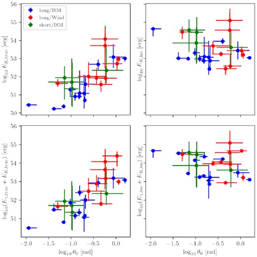
Scatter plot of (EK,iso, EK,true) and (Etotal,iso, Etotal,true) w.r.t. the inferred opening angles for the GRB sample. The blue circles and red diamonds represent long GRBs in homogeneous and wind-like environments, respectively. Error bars represent the 68 per cent credible interval.
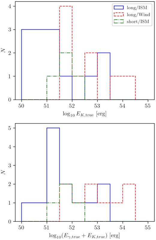
Histogram of the inferred energetics for the GRB sample. The upper and lower panels show the histograms for the EK,true and Etrue distributions, respectively.
We present the relevant derived parameters of the GRB sample in Table 6. In Fig. 8, it can be seen that short GRBs are systematically less efficient than long GRBs. The average value of the inferred ϵγ parameters for short and long GRBs are 2.7 × 10⁻⁴ and 0.26, respectively. Beniamini et al. (2015) have analysed the observed flux from 10 long GRBs in X-rays and GeV energies to estimate the energetics of these GRBs. They find that there is a discrepancy between the estimated energies using both bands, where the energy estimated from the GeV flux is significantly larger. They state that this discrepancy can be explained within the forward shock framework by either assuming that the cooling break lies between these two bands or by taking into account Compton cooling effects. As a result they find that the average prompt efficiency value becomes 0.87 for the X-ray estimated energies, and 0.14 for GeV estimated energies. They note that the GeV estimated energetics should be more reliable, and these are consistent with our results. We perform a KS test to determine if the ϵγ distribution for long and short GRBs originate from a common distribution. We find that the null hypothesis can be significantly rejected, with p = 1.3 × 10⁻⁴, so short GRBs are indeed less efficient gamma-ray emitters. However, this analysis does not account for the uncertainties in the ϵγ parameter, and relies only on the mode of the posterior distribution.
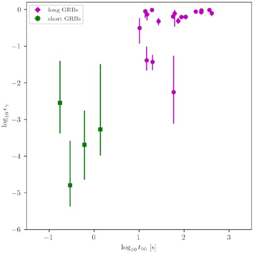
Scatter plot of the reported t90 and derived ϵγ parameters for the short and long GRB samples. The magenta circles and green squares represent long and short GRBs, respectively. Error bars represent the 68 per cent credible interval.
It is not so clear what might cause this difference in efficiency, and our study does not speak much to this because we examine only the physics of the afterglow. We do note that in the afterglow, the short GRB blast waves have a lower (synchrotron) emission efficiency, because this scales as ϵeϵB, which is lower on average for short GRBs (which have about the same ϵe and lower ϵB for a given true energy – see below). Whether we should expect that same difference to exist for the internal shocks that cause the prompt emission (or whether those are even dominated by synchrotron emission) is unclear, however. In Gottlieb, Levinson & Nakar (2019), the authors find that the main factor determining the radiative efficiency is the amount of baryon loading. Since our findings indicate that short GRBs are less efficient, this could also mean that baryon loading in short GRB jets is more prominent. Gottlieb et al. (2021a, see also Gottlieb, Levinson & Nakar 2020; Gottlieb, Nakar & Bromberg 2021b) have performed relativistic magnetohydrodynamic (RMHD) simulations to investigate how the prompt emission features (variability, spectrum and efficiency) vary for hydrodynamic and magnetized jets for both intermittent and continuous central engine activity scenarios. They have found that magnetized + intermittent jets are the most likely candidate for GRBs, as they yield high prompt efficiencies and are consistent with observed spectral and temporal features. They also note that, for hydrodynamic + intermittent jets, the efficiency drops below 1 per cent. As the degree of magnetization increases the mixing processes become less efficient and lead to higher ϵγ values.
In Tables 5 and 6, it can be seen that, in some cases, the derived values for the microphysical parameters are difficult to reconcile with our theoretical understanding (i.e. ϵB + ϵe ∼ 1). However, as mentioned previously, due to the ξN degeneracy these values can be scaled down to more reasonable values by assuming a smaller value for ξN. This is supported by particle-in-cell simulations which indicate that ξN can be as small as 0.01 (Sironi & Spitkovsky 2011). We find that the derived values for the prompt efficiencies, ϵγ, is approaching unity in some cases, which can be resolved by once again assuming a lower value for ξN to scale down the values for the prompt efficiency. Moreover, even if we lower the ξN value, assuming that the ϵe value is the same for both the prompt and afterglow phases, some of the modelling results suggest ϵγ > ϵe. Such high efficiencies are consistent with the proposed scenario by Kobayashi & Sari (2001).
Wang et al. (2018) have analysed the optical and X-ray light curves of a large sample of GRBs to determine any achromatic jet-breaks present in the data sets. They infer the energetics and the opening angle of the GRB sample by assuming fiducial values for the other GRB parameters and by making use of analytical prescriptions. They find that the energetics are distributed as log10EK,iso = 54.82 ± 0.56 and log10EK,true = 51.33 ± 0.58 for the long GRB population. In our analysis, we find log10EK,iso = 53.38 ± 0.72 and log10EK,true = 51.81 ± 1.08 for the long GRB population. We find that the energetics exhibit a wider spread across the long GRB population. We also find lower values for the mean of the EK,iso distribution. Since Wang et al. (2018) only consider GRBs with an observed achromatic jet-break, their selection effects are different than our sample.
4.3 ϵB–EK,true, θ0–ϵB anticorrelations
We find that θ0 and EK,true are strongly correlated with each other for both wind-like and ISM-like long GRBs; this does not, however, have any new meaning. It is simply the result of the fact that Etrue is derived from Eiso via the opening angle, and that the distribution of Eiso is fairly narrow, whereas that of θ0 is wider. Hence, this correlation is largely due to the fact that we are correlating θ0 with itself.
We do however find a strong and significant anticorrelation between ϵB and EK,true for the sample of long GRBs. In Fig. 9, we demonstrate this anticorrelation. We find that the fraction of energy lost to amplifying magnetic fields systematically decreases as the measured beaming corrected kinetic energy gets larger. When we perform a Pearson r correlation test we find a p-value of 10−5, strongly rejecting the null hypothesis that they are uncorrelated. Alternatively, we can of course regard this correlation as due to an ϵB−θ0 relation. We also checked for a possible correlation between ϵB and EK,iso; it is not significant. This may be somewhat surprising, since we think of the energy fractions in electrons and magnetic field to be set very locally at the shock, and thus correlate better with EK,iso, which scales with the local energy per unit area at the shock.
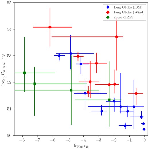
Scatter plot of ϵB and EK,true parameters for the GRB sample. The blue circles, red diamonds, and green squares represent ISM-like long GRBs, wind-like long GRBs and short GRBs, respectively. Error bars represent the 68 per cent credible interval.
Since the number of GRBs in either sample is small, we use a Jackknife resampling test to check the robustness of these correlations due to outliers. The results can be seen in Table 7, and show that the significant correlations are robust. However, they also reveal are rather strong difference between the two subclasses: the correlations are not significant in the wind-like GRBs and very strongly significant in the ISM-likes. The significance of the result for the total population is therefore entirely due to that of the ISM-like GRBs. This is puzzling, since it unclear how the correlation between these two blast wave parameters would come to depend on the shape of the ambient density distribution.
Correlation significance results for the Jackknife re-sampling. The upper panel shows p-value estimates for the whole long GRB sample, the middle panel takes into account only the long GRBs in ISM-like environments, and the bottom panel is for the long GRBs in wind-like environments.
| Anti-/correlation | p-value | |||
|---|---|---|---|---|
| Minimum | Maximum | Average | ||
| Long GRBs | ϵB-EK,true | 1.22 × 10⁻⁷ | 2.28 × 10⁻⁴ | 4.65 × 10⁻⁵ |
| θ0-ϵB | 6.85 × 10⁻⁴ | 0.010 | 4.18 × 10⁻³ | |
| ϵB-EK,iso | 0.011 | 0.48 | 0.12 | |
| ISM-like | ϵB-EK,true | 4.74 × 10⁻⁶ | 1.28 × 10⁻⁴ | 3.66 × 10⁻⁵ |
| θ0-ϵB | 1.71 × 10⁻⁴ | 6.12 × 10⁻³ | 1.60 × 10⁻³ | |
| ϵB-EK,iso | 0.10 | 0.99 | 0.82 | |
| Wind-like | ϵB-EK,true | 0.011 | 0.68 | 0.21 |
| θ0-ϵB | 0.55 | 0.99 | 0.87 | |
| ϵB-EK,iso | 9.03 × 10⁻³ | 0.37 | 0.12 | |
4.4 Caveats
First of all, it is not straightforward to infer population distributions from uncertain measurements. When creating histograms we only considered the point estimate (i.e. mode of the posterior distribution) of the inferred parameter values. This approach does not take into account the full information contained in the obtained parameter distributions. It would be valuable to combine the posterior distributions from individual modelling efforts to estimate how the parameters are distributed across the GRB population in a statistically correct manner (e.g. Mandel 2010; Hogg, Myers & Bovy 2010); however, this is out of the scope of this work.
Secondly, it is not possible to compile an unbiased sample of well-sampled afterglows, because a variety of instrumental biases and observer choices enter into the determination of which GRBs to follow up extensively and for which such follow-up is successful. Therefore, the inferred GRB population will likely not cover all of the physical parameter space. We have commented above on whether we estimate this has a significant influence on our conclusions. While we accounted for the small sample size of especially short GRBs when stating significances, it is still good to bear in mind that our short GRBs are especially unrepresentative of the total population of short GRBs (though, as we noted, there is no clear expectation that this this would bias the intrinsic properties of this subset of short GRBs, for which we draw the most marked conclusions).
5 CONCLUSION
We have studied a sample of 26 GRB afterglows (as well as the total prompt gamma-ray energy emitted), which was biased to enabling detailed afterglow physics studies, i.e. towards having well-sampled radio, optical, and X-ray light curves. While this largely excludes the most obscured GRBs (due to optical extinction) and GRBs in low-density regions (i.e. most short GRBs), we argue that there are quite a few conclusions about GRB physics that are not strongly affected by those biases:
All physical parameters have intrinsic distributions of significant width, i.e. none have a ‘standard’ value that is almost the same for all GRBs, or even within a subsample (short, long-ISM, or long-wind; Section 3).
Short GRBs prefer uniform ambient densities, in agreement with theoretical expectations and previous studies (Section 3.1).
Long GRBs have about equal likelihood of wind-like and uniform ambient media. A massive star progenitor is expected to impact the environment of the burst, suggesting a wind-like medium to be more likely. We note that even a massive star wind environment can be close to homogeneous at scales probed by the afterglow observations, but that this is not the most natural outcome for typical parameters (Section 4.1).
The wind strengths for the wind-like long GRBs favour canonical mass-loss parameters of massive Wolf–Rayet stars, the most likely progenitors, and specifically do not indicate a bias towards low mass-loss rates, as required by some GRB models (Section 4.1).
We do not find evidence for different jet opening angles between long and short GRBs (Section 3.2).
The observer viewing angles are consistent with top-hat jets, and with the opening angles of the prompt gamma-ray emission and early afterglow emission being the same.
We find a distribution of slopes of the energy distribution of accelerated electrons, p, that is consistent with previous studies; it contains only a few examples where p < 2 significantly, but many where it is close enough to 2 to warrant caution in fitting p and ϵe (Section 3.3).
The values of ϵe are all in the range of 0.1 – 1, with no significant differences between short/long or wind/uniform samples (Section 3.3).
The true total energies of long and short GRBs are similar, implying that the relative faintness of short GRBs in gamma-rays is due to their lower gamma-ray emission efficiency (Section 4.2).
Some required gamma-ray efficiencies of GRBs are close to 1, which is a challenging value for current prompt emission theories (Section 4.2).
There is a strong and significant correlation for ISM-like long GRBs between the magnetic field energy at the shock and the true total kinetic energy of the blast wave. It is surprising that this same correlation does not exist for the wind-like GRBs (Section 4.3).
SUPPORTING INFORMATION
Figure S1. Modelling results for GRB 970508 assuming homogeneous circumburst density profile. The plot on the left represents the posterior predictive light curves for 100 randomly sampled parameter sets from the posterior parameter distribution. The plot on the right represents the corner plot for the obtained posterior distribution from the Bayesian inference.
Figure S2. Modelling results for GRB 970508 assuming wind-like circumburst density profile. The plot on the left represents the posterior predictive light curves for 100 randomly sampled parameter sets from the posterior parameter distribution. The plot on the right represents the corner plot for the obtained posterior distribution from the Bayesian inference.
Figure S3. Modelling results for GRB 980703 assuming homogeneous circumburst density profile. The plot on the left represents the posterior predictive light curves for 100 randomly sampled parameter sets from the posterior parameter distribution. The plot on the right represents the corner plot for the obtained posterior distribution from the Bayesian inference.
Figure S4. Modelling results for GRB 980703 assuming wind-like circumburst density profile. The plot on the left represents the posterior predictive light curves for 100 randomly sampled parameter sets from the posterior parameter distribution. The plot on the right represents the corner plot for the obtained posterior distribution from the Bayesian inference.
Figure S5. Modelling results for GRB 990510 assuming homogeneous circumburst density profile. The plot on the left represents the posterior predictive light curves for 100 randomly sampled parameter sets from the posterior parameter distribution. The plot on the right represents the corner plot for the obtained posterior distribution from the Bayesian inference.
Figure S6. Modelling results for GRB 990510 assuming wind-like circumburst density profile. The plot on the left represents the posterior predictive light curves for 100 randomly sampled parameter sets from the posterior parameter distribution. The plot on the right represents the corner plot for the obtained posterior distribution from the Bayesian inference.
Figure S7. Modelling results for GRB 991208 assuming homogeneous circumburst density profile. The plot on the left represents the posterior predictive light curves for 100 randomly sampled parameter sets from the posterior parameter distribution. The plot on the right represents the corner plot for the obtained posterior distribution from the Bayesian inference.
Figure S8. Modelling results for GRB 991208 assuming wind-like circumburst density profile. The plot on the left represents the posterior predictive light curves for 100 randomly sampled parameter sets from the posterior parameter distribution. The plot on the right represents the corner plot for the obtained posterior distribution from the Bayesian inference.
Figure S9. Modelling results for GRB 991216 assuming homogeneous circumburst density profile. The plot on the left represents the posterior predictive light curves for 100 randomly sampled parameter sets from the posterior parameter distribution. The plot on the right represents the corner plot for the obtained posterior distribution from the Bayesian inference.
Figure S10. Modelling results for GRB 991216 assuming wind-like circumburst density profile. The plot on the left represents the posterior predictive light curves for 100 randomly sampled parameter sets from the posterior parameter distribution. The plot on the right represents the corner plot for the obtained posterior distribution from the Bayesian inference.
Figure S11. Modelling results for GRB 000301C assuming homogeneous circumburst density profile. The plot on the left represents the posterior predictive light curves for 100 randomly sampled parameter sets from the posterior parameter distribution. The plot on the right represents the corner plot for the obtained posterior distribution from the Bayesian inference.
Figure S12. Modelling results for GRB 000301C assuming wind-like circumburst density profile. The plot on the left represents the posterior predictive light curves for 100 randomly sampled parameter sets from the posterior parameter distribution. The plot on the right represents the corner plot for the obtained posterior distribution from the Bayesian inference.
Figure S13. Modelling results for GRB 000418 assuming homogeneous circumburst density profile. The plot on the left represents the posterior predictive light curves for 100 randomly sampled parameter sets from the posterior parameter distribution. The plot on the right represents the corner plot for the obtained posterior distribution from the Bayesian inference.
Figure S14. Modelling results for GRB 000418 assuming wind-like circumburst density profile. The plot on the left represents the posterior predictive light curves for 100 randomly sampled parameter sets from the posterior parameter distribution. The plot on the right represents the corner plot for the obtained posterior distribution from the Bayesian inference.
Figure S15. Modelling results for GRB 000926 assuming homogeneous circumburst density profile. The plot on the left represents the posterior predictive light curves for 100 randomly sampled parameter sets from the posterior parameter distribution. The plot on the right represents the corner plot for the obtained posterior distribution from the Bayesian inference.
Figure S16. Modelling results for GRB 000926 assuming wind-like circumburst density profile. The plot on the left represents the posterior predictive light curves for 100 randomly sampled parameter sets from the posterior parameter distribution. The plot on the right represents the corner plot for the obtained posterior distribution from the Bayesian inference.
Figure S17. Modelling results for GRB 010222 assuming homogeneous circumburst density profile. The plot on the left represents the posterior predictive light curves for 100 randomly sampled parameter sets from the posterior parameter distribution. The plot on the right represents the corner plot for the obtained posterior distribution from the Bayesian inference.
Figure S18. Modelling results for GRB 010222 assuming wind-like circumburst density profile. The plot on the left represents the posterior predictive light curves for 100 randomly sampled parameter sets from the posterior parameter distribution. The plot on the right represents the corner plot for the obtained posterior distribution from the Bayesian inference.
Figure S19. Modelling results for GRB 030329 assuming homogeneous circumburst density profile. The plot on the left represents the posterior predictive light curves for 100 randomly sampled parameter sets from the posterior parameter distribution. The plot on the right represents the corner plot for the obtained posterior distribution from the Bayesian inference.
Figure S20. Modelling results for GRB 030329 assuming wind-like circumburst density profile. The plot on the left represents the posterior predictive light curves for 100 randomly sampled parameter sets from the posterior parameter distribution. The plot on the right represents the corner plot for the obtained posterior distribution from the Bayesian inference.
Figure S21. Modelling results for GRB 050820A assuming homogeneous circumburst density profile. The plot on the left represents the posterior predictive light curves for 100 randomly sampled parameter sets from the posterior parameter distribution. The plot on the right represents the corner plot for the obtained posterior distribution from the Bayesian inference.
Figure S22. Modelling results for GRB 050820A assuming wind-like circumburst density profile. The plot on the left represents the posterior predictive light curves for 100 randomly sampled parameter sets from the posterior parameter distribution. The plot on the right represents the corner plot for the obtained posterior distribution from the Bayesian inference.
Figure S23. Modelling results for GRB 050904 assuming homogeneous circumburst density profile. The plot on the left represents the posterior predictive light curves for 100 randomly sampled parameter sets from the posterior parameter distribution. The plot on the right represents the corner plot for the obtained posterior distribution from the Bayesian inference.
Figure S24. Modelling results for GRB 050904 assuming wind-like circumburst density profile. The plot on the left represents the posterior predictive light curves for 100 randomly sampled parameter sets from the posterior parameter distribution. The plot on the right represents the corner plot for the obtained posterior distribution from the Bayesian inference.
Figure S25. Modelling results for GRB 051221A assuming homogeneous circumburst density profile. The plot on the left represents the posterior predictive light curves for 100 randomly sampled parameter sets from the posterior parameter distribution. The plot on the right represents the corner plot for the obtained posterior distribution from the Bayesian inference.
Figure S26. Modelling results for GRB 051221A assuming wind-like circumburst density profile. The plot on the left represents the posterior predictive light curves for 100 randomly sampled parameter sets from the posterior parameter distribution. The plot on the right represents the corner plot for the obtained posterior distribution from the Bayesian inference.
Figure S27. Modelling results for GRB 060418 assuming homogeneous circumburst density profile. The plot on the left represents the posterior predictive light curves for 100 randomly sampled parameter sets from the posterior parameter distribution. The plot on the right represents the corner plot for the obtained posterior distribution from the Bayesian inference.
Figure S28. Modelling results for GRB 060418 assuming wind-like circumburst density profile. The plot on the left represents the posterior predictive light curves for 100 randomly sampled parameter sets from the posterior parameter distribution. The plot on the right represents the corner plot for the obtained posterior distribution from the Bayesian inference.
Figure S29. Modelling results for GRB 090328 assuming homogeneous circumburst density profile. The plot on the left represents the posterior predictive light curves for 100 randomly sampled parameter sets from the posterior parameter distribution. The plot on the right represents the corner plot for the obtained posterior distribution from the Bayesian inference.
Figure S30. Modelling results for GRB 090328 assuming wind-like circumburst density profile. The plot on the left represents the posterior predictive light curves for 100 randomly sampled parameter sets from the posterior parameter distribution. The plot on the right represents the corner plot for the obtained posterior distribution from the Bayesian inference.
Figure S31. Modelling results for GRB 090423 assuming homogeneous circumburst density profile. The plot on the left represents the posterior predictive light curves for 100 randomly sampled parameter sets from the posterior parameter distribution. The plot on the right represents the corner plot for the obtained posterior distribution from the Bayesian inference.
Figure S32. Modelling results for GRB 090423 assuming wind-like circumburst density profile. The plot on the left represents the posterior predictive light curves for 100 randomly sampled parameter sets from the posterior parameter distribution. The plot on the right represents the corner plot for the obtained posterior distribution from the Bayesian inference.
Figure S33. Modelling results for GRB 090902B assuming homogeneous circumburst density profile. The plot on the left represents the posterior predictive light curves for 100 randomly sampled parameter sets from the posterior parameter distribution. The plot on the right represents the corner plot for the obtained posterior distribution from the Bayesian inference.
Figure S34. Modelling results for GRB 090902B assuming wind-like circumburst density profile. The plot on the left represents the posterior predictive light curves for 100 randomly sampled parameter sets from the posterior parameter distribution. The plot on the right represents the corner plot for the obtained posterior distribution from the Bayesian inference.
Figure S35. Modelling results for GRB 090926A assuming homogeneous circumburst density profile. The plot on the left represents the posterior predictive light curves for 100 randomly sampled parameter sets from the posterior parameter distribution. The plot on the right represents the corner plot for the obtained posterior distribution from the Bayesian inference.
Figure S36. Modelling results for GRB 090926A assuming wind-like circumburst density profile. The plot on the left represents the posterior predictive light curves for 100 randomly sampled parameter sets from the posterior parameter distribution. The plot on the right represents the corner plot for the obtained posterior distribution from the Bayesian inference.
Figure S37. Modelling results for GRB 120521C assuming homogeneous circumburst density profile. The plot on the left represents the posterior predictive light curves for 100 randomly sampled parameter sets from the posterior parameter distribution. The plot on the right represents the corner plot for the obtained posterior distribution from the Bayesian inference.
Figure S38. Modelling results for GRB 120521C assuming wind-like circumburst density profile. The plot on the left represents the posterior predictive light curves for 100 randomly sampled parameter sets from the posterior parameter distribution. The plot on the right represents the corner plot for the obtained posterior distribution from the Bayesian inference.
Figure S39. Modelling results for GRB 130427A assuming homogeneous circumburst density profile. The plot on the left represents the posterior predictive light curves for 100 randomly sampled parameter sets from the posterior parameter distribution. The plot on the right represents the corner plot for the obtained posterior distribution from the Bayesian inference.
Figure S40. Modelling results for GRB 130427A assuming wind-like circumburst density profile. The plot on the left represents the posterior predictive light curves for 100 randomly sampled parameter sets from the posterior parameter distribution. The plot on the right represents the corner plot for the obtained posterior distribution from the Bayesian inference.
Figure S41. Modelling results for GRB 130603B assuming homogeneous circumburst density profile. The plot on the left represents the posterior predictive light curves for 100 randomly sampled parameter sets from the posterior parameter distribution. The plot on the right represents the corner plot for the obtained posterior distribution from the Bayesian inference.
Figure S42. Modelling results for GRB 130603B assuming wind-like circumburst density profile. The plot on the left represents the posterior predictive light curves for 100 randomly sampled parameter sets from the posterior parameter distribution. The plot on the right represents the corner plot for the obtained posterior distribution from the Bayesian inference.
Figure S43. Modelling results for GRB 130702A assuming homogeneous circumburst density profile. The plot on the left represents the posterior predictive light curves for 100 randomly sampled parameter sets from the posterior parameter distribution. The plot on the right represents the corner plot for the obtained posterior distribution from the Bayesian inference.
Figure S44. Modelling results for GRB 130702A assuming wind-like circumburst density profile. The plot on the left represents the posterior predictive light curves for 100 randomly sampled parameter sets from the posterior parameter distribution. The plot on the right represents the corner plot for the obtained posterior distribution from the Bayesian inference.
Figure S45. Modelling results for GRB 130907A assuming homogeneous circumburst density profile. The plot on the left represents the posterior predictive light curves for 100 randomly sampled parameter sets from the posterior parameter distribution. The plot on the right represents the corner plot for the obtained posterior distribution from the Bayesian inference.
Figure S46. Modelling results for GRB 130907A assuming wind-like circumburst density profile. The plot on the left represents the posterior predictive light curves for 100 randomly sampled parameter sets from the posterior parameter distribution. The plot on the right represents the corner plot for the obtained posterior distribution from the Bayesian inference.
Figure S47. Modelling results for GRB 140304A assuming homogeneous circumburst density profile. The plot on the left represents the posterior predictive light curves for 100 randomly sampled parameter sets from the posterior parameter distribution. The plot on the right represents the corner plot for the obtained posterior distribution from the Bayesian inference.
Figure S48. Modelling results for GRB 140304A assuming wind-like circumburst density profile. The plot on the left represents the posterior predictive light curves for 100 randomly sampled parameter sets from the posterior parameter distribution. The plot on the right represents the corner plot for the obtained posterior distribution from the Bayesian inference.
Figure S49. Modelling results for GRB 140903A assuming homogeneous circumburst density profile. The plot on the left represents the posterior predictive light curves for 100 randomly sampled parameter sets from the posterior parameter distribution. The plot on the right represents the corner plot for the obtained posterior distribution from the Bayesian inference.
Figure S50. Modelling results for GRB 140903A assuming wind-like circumburst density profile. The plot on the left represents the posterior predictive light curves for 100 randomly sampled parameter sets from the posterior parameter distribution. The plot on the right represents the corner plot for the obtained posterior distribution from the Bayesian inference.
Figure S51. Modelling results for GRB 200522A assuming homogeneous circumburst density profile. The plot on the left represents the posterior predictive light curves for 100 randomly sampled parameter sets from the posterior parameter distribution. The plot on the right represents the corner plot for the obtained posterior distribution from the Bayesian inference.
Figure S52. Modelling results for GRB 200522A assuming wind-like circumburst density profile. The plot on the left represents the posterior predictive light curves for 100 randomly sampled parameter sets from the posterior parameter distribution. The plot on the right represents the corner plot for the obtained posterior distribution from the Bayesian inference.
Please note: Oxford University Press is not responsible for the content or functionality of any supporting materials supplied by the authors. Any queries (other than missing material) should be directed to the corresponding author for the article.
ACKNOWLEDGEMENTS
We thank the anonymous referee for their insightful comments. This work was carried out on the Dutch national e-infrastructure with the support of SURF Cooperative. HJvE acknowledges partial support by the European Union Horizon 2020 Programme under the AHEAD2020 project (grant agreement number 871158).
DATA AVAILABILITY
A reproduction package including the data underlying this article will be made available at Zenodo with DOI: 10.5281/zenodo.5035173.
REFERENCES
APPENDIX: POSTERIOR DISTRIBUTIONS FOR THE FREE PHYSICAL PARAMETERS

Violin plots representing the obtained posterior distributions of the free physical parameters for the long GRB sample associated with a constant density environment. The shaded areas represent the density of the posterior samples and circles represent the mean value. Error bars represent the 68 per cent credible interval.
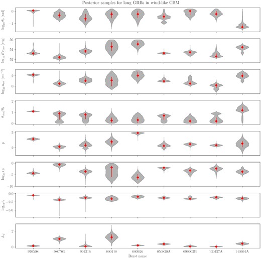
Violin plots representing the obtained posterior distributions of the free physical parameters for the long GRB sample associated with a wind-like environment. The shaded areas represent the density of the posterior samples and diamonds represent the mean value. Error bars represent the 68 per cent credible interval.
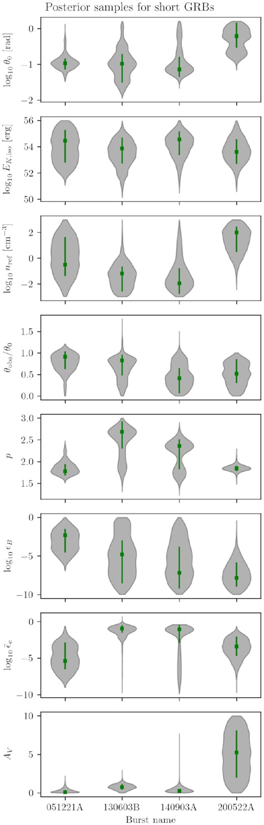
Violin plots representing the obtained posterior distributions of the free physical parameters for the short GRB sample. The shaded areas represent the density of the posterior samples and squares represent the mean value. Error bars represent the 68 per cent credible interval.
