Modelling nearest neighbour distributions of biased tracers using hybrid effective field theory

Banerjee, Arka; Kokron, Nickolas; Abel, Tom

doi:10.1093/mnras/stac193

ABSTRACT

We investigate the application of hybrid effective field theory (HEFT) – which combines a Lagrangian bias expansion with subsequent particle dynamics from N-body simulations – to the modelling of k-nearest neighbour cumulative distribution functions (kNN-CDFs) of biased tracers of the cosmological matter field. The kNN-CDFs are sensitive to all higher order connected N-point functions in the data, but are computationally cheap to compute. We develop the formalism to predict the kNN-CDFs of discrete tracers of a continuous field from the statistics of the continuous field itself. Using this formalism, we demonstrate how kNN-CDF statistics of a set of biased tracers, such as haloes or galaxies, of the cosmological matter field can be modelled given a set of low-redshift HEFT component fields and bias parameter values. These are the same ingredients needed to predict the two-point clustering. For a specific sample of haloes, we show that both the two-point clustering and the kNN-CDFs can be well-fit on quasi-linear scales (≳ 20h⁻¹Mpc) by the second-order HEFT formalism with the same values of the bias parameters, implying that joint modelling of the two is possible. Finally, using a Fisher matrix analysis, we show that including kNN-CDF measurements over the range of allowed scales in the HEFT framework can improve the constraints on σ₈ by roughly a factor of 3, compared to the case where only two-point measurements are considered. Combining the statistical power of kNN measurements with the modelling power of HEFT, therefore, represents an exciting prospect for extracting greater information from small-scale cosmological clustering.

cosmological parameters, large-scale structure of Universe

1 INTRODUCTION

Various cosmological surveys, both current such as EBOSS, DES, and KiDS (see Alam et al. 2021; DES Collaboration et al. 2021; Heymans et al. 2021) and upcoming ones, including LSST, Euclid, SPHEREx, WFIRST, DESI, and PFS (Laureijs et al. 2011; Doré et al. 2014; Takada et al. 2014; DESI Collaboration et al. 2016; Dore et al. 2019; Ivezić et al. 2019), are in the process of mapping out the clustering of tracers of structure in the Universe, such as galaxies, in progressively greater detail. This data can be used to answer various fundamental questions, such as the equation of state of dark energy, the nature of dark matter, and total mass of the standard model neutrinos. Much progress has been made on this front in the last few decades, using the clustering of structure on large scales, where linear perturbation theory (in the density contrast) provides an accurate framework. The next challenge is to model clustering on smaller scales – where linear perturbation theory breaks down – and thereby extract maximal information from the data provided by these surveys. It should also be noted that once the underlying cosmological matter field is no longer linear, the approximation that it is a Gaussian random field breaks down. This implies that the two-point correlation function, which is the complete statistical description of a Gaussian random field, does not characterize the field completely. Therefore, the challenge of extracting useful information on the cosmological parameters of interest from small-scale clustering is intimately connected to characterizing clustering beyond the two-point correlations (Gruen et al. 2015; Hahn et al. 2020; Uhlemann et al. 2020; Chen, Lee & Dvorkin 2021; Hahn & Villaescusa-Navarro 2021).

One approach to the goal of harnessing smaller scale information is through the use of N-body simulations (Hockney & Eastwood 1988), which accurately model the late-time clustering of the cold dark matter (CDM) component of the Universe down to small and extremely non-linear scales (see e.g. Heitmann et al. 2005, 2008). However, these simulations do not capture the evolution of the baryonic component of the Universe, and therefore, do not by themselves predict the clustering of visible tracers of structure, like galaxies, that are observed by cosmological surveys. To connect the outputs of the numerical simulations and observations, an additional layer of modelling, i.e. the tracer–matter connection is needed, and various such prescriptions exist in the literature (see Wechsler & Tinker 2018 for an extensive review). One of the most popular models, especially to model clustering of tracers on intermediate, quasi-linear scales, is the generic bias expansion (see Desjacques, Jeong & Schmidt 2018 for a review of these models). In particular, the Lagrangian bias formalism (Matsubara 2008b) connects the late-time clustering of biased tracers to properties of the initial distribution of the underlying matter field. Traditionally, the Lagrangian bias approach has been coupled with perturbation theory approaches to computing the displacement field connecting the early and late time matter fields. An analytic prescription for displacements results in the well-known Lagrangian Perturbation Theory (Matsubara 2008a, b). Extending the model to include counter-terms due to small-scale dynamics leads to Lagrangian Effective Field Theory (Porto, Senatore & Zaldarriaga 2014; Vlah, White & Aviles 2015). Other recent developments include formulations of LPT which partially re-sum contributions while preserving Galilean invariance, leading to Convolution Lagrangian Effective Field Theory (Carlson, Reid & White 2012; Vlah, Castorina & White 2016).

Perturbative approaches have been developed over the years to improve models both tracer–tracer and tracer–matter two-point clustering. In particular, Eulerian approaches to modelling two-point clustering have recently been successfully applied to the analysis of the Baryon Oscillation Spectroscopic Survey (BOSS)¹ data (d’Amico et al. 2020; Ivanov, Simonović & Zaldarriaga 2020). These studies represented the first analyses to use the full shape information for the two-point clustering of the BOSS data, down to scales of |$k_{\rm max} \simeq 0.25\, h {\rm Mpc}^{-1}$|⁠. Despite the tremendous advances in perturbative modelling, it is known that by themselves they cannot be used to extract all of the small-scale information contained in the galaxy density field. Perturbative models are best suited to the scales mentioned above (⁠|$k\sim 0.25 \, h{\rm Mpc}^{-1}$|⁠), which in the next-generation of spectroscopic surveys such as DESI will be probed with unparalleled volumes and statistical power. Nevertheless, the amount of potential cosmological information contained within correlations on even smaller scales will potentially be even higher. This motivates models that can accurately predict the statistics of tracers down to scales smaller than what can be achieved purely via perturbation theory.

As a way to combine the generality of Lagrangian bias models with smaller scale information, Modi, Chen & White (2020) demonstrated that using the displacement field from N-body simulations, which accounts for the full gravitational evolution down to non-linear scales, can increase the range of scales over which the two-point clustering of biased tracers is well described for the same order of Lagrangian bias expansion. This was found to be especially true for moderately biased tracers at low redshifts, where the model worked well up to |$k_{\rm max} \sim 0.6 \, h{\rm Mpc}^{-1}$|⁠, nearly doubling the range of scales from perturbation theory approaches. This approach, hybrid effective field theory (HEFT), has since been merged with an emulator framework (Kokron et al. 2021; Zennaro et al. 2021), and recently applied to data (Hadzhiyska et al. 2021). While the existing studies all focused on two-point clustering, the model applies the bias expansion at the field level, and then uses N-body evolution to compute the advected fields. The late-time non-linear component fields themselves are natural predictions of this model, rather than any particular statistics over these fields. Therefore, it is of great interest to assess their ability in capturing more complex summary statistics of tracers than just their two-point functions. Given a set of bias coefficients in HEFT, the fields should also model higher order statistics (such as the bispectrum and trispectrum) of the tracer population. This was explored, for a similar model to HEFT, in the context of halo samples in Schmittfull et al. (2019) and for redshift-space samples of galaxies in Schmittfull et al. (2021). Nevertheless, the computational complexity of N > two-point analyses is quite large (however, see Philcox & Slepian 2021 for recent progress in this direction), and so we seek an alternative summary statistic that encodes higher order information, to test the applicability of HEFT.

Banerjee & Abel (2021a, 2021b) have proposed a set of new summary statistics to capture the auto and joint clustering of various tracer samples in the context of cosmology. These statistics, the k-Nearest Neighbour Cumulative Distribution Functions (kNN-CDFs) are constructed by considering the distribution of distances to the k-th nearest data point from a volume-spanning set of query points. If the tracers represent a local Poisson sampling of an underlying field, the kNN-CDFs are sensitive to integrals of all connected N-point functions of the underlying field. For two sets of tracers, and their corresponding underlying fields, Banerjee & Abel (2021b) demonstrated that the joint kNN-CDFs are sensitive to all combinations of N-point functions that can be formed from the two fields. This makes these statistics a powerful probe of clustering, and was recently applied to the measurement of the clustering of very massive galaxy clusters (Wang, Banerjee & Abel 2021). At the same time, these statistics are particularly easy to compute on a given data set, taking orders of magnitude lower computational resources compared to other statistical measures of clustering beyond the two-point function. These attractive features make these statistics a promising candidate to apply to cosmological data sets from surveys, especially to galaxy clustering. However, while the kNN distributions are statistically powerful characterizations the clustering of a set of galaxies (tracers), the final goal is to extract the cosmological parameters of interest in an unbiased manner. This can only be done after marginalizing over an appropriate set parameters that model the a priori unknown connection between the underlying matter field, that is controlled by the cosmological parameters, and the galaxies that are observed. In other words, the tracer–matter connection needs to be understood in the language of these statistics in order to enable their application to data.

In this paper, we investigate the use of the HEFT framework as the model of the tracer–matter connection for kNN statistics. At the same time, this paper also represents the first application of the HEFT framework to any statistics beyond the two-point function. The paper is organized as follows: In Section 2, we develop the formalism for predicting the kNN-CDFs of a set of discrete tracers of a clustered, continuous field in terms of the statistical properties of the field itself. We also provide a concrete implementation of the formalism for the case where the tracers are a random subset of particles from a cosmological N-body simulation, and the underlying field is the matter field at that redshift. In Section 3, we give a brief introduction to the HEFT framework, and outline how to compute kNN distributions of biased tracers from the ‘weight’ fields generated by the HEFT formalism. In Section 4, we choose a halo sample, whose mass range is roughly representative of the luminous red galaxy (LRG) sample hosts at z = 0.5, from simulations and fit its kNN distributions using the formalism from Section 3. We identify a set of scales over which HEFT is an accurate description of the tracer–matter connection for various kNN distributions. We also demonstrate that there are a set of bias values which can jointly model both the two-point clustering and the kNN distributions of the halo sample. In Section 5, we use a Fisher matrix formalism to estimate the potential gains in cosmological parameter constraints within the HEFT framework when kNN measurements are considered in addition to the traditional two-point measurements. We summarize the main points of our findings, and discuss certain interesting features of the study in Section 6.

2 FORMALISM AND CALCULATION FRAMEWORK

In this section, we will lay out the formalism for making predictions for the kNN-CDF measurements of discrete tracers from the properties of a continuous underlying field, assuming the tracers represent a Poisson sampling of the underlying field (see Banerjee & Abel 2021a for details). Having laid out the formalism for a general field, we will demonstrate its application to the prediction of kNN-CDF of a set of simulation particles with mean number density |$\bar{n}$| given the continuous underlying matter field in Section 2.1.

The general setup is that of N tracer (data) points, whose clustering we want to characterize, distributed over a total volume V_tot. To compute the nearest neighbour distribution, the same volume is densely populated with a set of query points, and the distances to the k-nearest data point is measured from each query point. These distances, for a specific value of k, are then sorted to calculate the Empirical CDF of the distribution of distances to the k-th nearest neighbour data points. These measurements, while sensitive to higher order N-point functions, are computationally much cheaper than those typically used to measure information beyond two-point clustering. As shown in Banerjee & Abel (2021a), the value of the CDF of the k-th nearest neighbour distribution at radius r is equal to the probability of finding more than k − 1 tracers in a spherical volume V = 4/3|$\pi$|r³:

$$\begin{eqnarray} {\rm CDF}_{k}(r) = \mathcal {P}_{\gt k-1}(V) = 1 - \Big (\mathcal {P}_0(V) + \ldots + \mathcal {P}_{k}(V)\Big)\, , \end{eqnarray}$$

(1)

where |$\mathcal {P}_k(V)$| is the probability of finding k tracers in a volume V. Note that these probabilities are averaged over the entire volume of interest.

If the tracers represent a Poisson sampling of an underlying continuous field |$\rho ({\boldsymbol x})$|⁠, then the probability of finding k tracers in a sphere of radius r around a specific point |${\boldsymbol x}_i$| is given by

$$\begin{eqnarray} \mathcal {P}_k(V)|_{{\boldsymbol x}_i} = \frac{\Big (M\left({\boldsymbol x}_i,V\right)/m\Big)^k}{k!}\exp \Big [-M\left({\boldsymbol x}_i,V\right)/m\Big ]\, , \end{eqnarray}$$

(2)

where

$$\begin{eqnarray} M({\boldsymbol x}_i,V) = \int _{|{\boldsymbol x}- {\boldsymbol x}_i|\lt R}\rho ({\boldsymbol x}) {\rm d}^3{\boldsymbol x}\, , \end{eqnarray}$$

(3)

or the total ‘mass’ in the sphere of radius R around point |${\boldsymbol x}_i$|⁠. m represents the ‘mass’ of each tracer. Note that the ratio of M/m is dimensionless. The volume-averaged probability |$\mathcal {P}_k(V)$| can be expressed as

$$\begin{eqnarray} \mathcal {P}_k(V) = \Big \langle \mathcal {P}_k(V)|_{{\boldsymbol x}_i}\Big \rangle \, , \end{eqnarray}$$

(4)

where the average runs over all possible positions, |${\boldsymbol x}_i$| for the centre of the sphere. As shown in Banerjee & Abel (2021a), |$\mathcal {P}_k(V)$| can also be formally expressed in terms of all connected N-point functions, |$\xi ^{(N)}({\boldsymbol r}_1,\ldots,{\boldsymbol r}_N)$|⁠, of the underlying field,

$$\begin{eqnarray} \mathcal {P}_k(V) &=& \frac{1}{k!}\Bigg [\Bigg (\frac{\rm d}{\rm d z}\Bigg)^k\exp \Bigg [\sum _{N=0}^{\infty }\frac{\bar{n}^N(z-1)^N}{N!}\\ && \times \, \int _V\ldots\int _V {\rm d}^3{\boldsymbol r}_1\ldots{\rm d}^3{\boldsymbol r}_N\xi ^{(N)}({\boldsymbol r}_1\ldots {\boldsymbol r}_N)\Bigg ]\Bigg ]_{z=0}\, , \end{eqnarray}$$

(5)

where |$\bar{n}$| is the mean number density of the tracers.

Combining equations (1), (2), and (4), the expression for value of the first three kNN-CDF at some radius r (or corresponding volume V) can be written as

$$\begin{eqnarray} {\rm CDF}_{1{\rm NN}} & = 1 - \Big \langle \exp \left[-\lambda _i\right]\Big \rangle, \end{eqnarray}$$

(6)

$$\begin{eqnarray} {\rm CDF}_{2{\rm NN}} & = 1 - \Big \langle \exp \left[-\lambda _i\right]\Big \rangle - \Big \langle \lambda _i \exp \left[-\lambda _i\right]\Big \rangle, \end{eqnarray}$$

(7)

$$\begin{eqnarray} {\rm CDF}_{3{\rm NN}} &=& 1 - \Big \langle \exp \left[-\lambda _i\right]\Big \rangle - \Big \langle \lambda _i \exp \left[-\lambda _i\right]\Big \rangle \\ &&- \frac{1}{2} \Big \langle \lambda _i^2 \exp \left[-\lambda _i\right]\Big \rangle \, , \end{eqnarray}$$

(8)

where |$\lambda _i = M({\boldsymbol x}_i, V)/m$|⁠. From equation (5), it is clear that each kNN-CDF measurement is sensitive to a different combination of the integrals of various N-point functions of the underlying field.

Banerjee & Abel (2021b) demonstrated the extension of the kNN framework to the joint CDFs of two sets of tracers – N₁ tracers of type 1 and N₂ tracers of type 2 distributed over a total volume V_tot. The joint |${\rm CDF}_{k_1,k_2}$| is computed by measuring the distances to the k₁th nearest neighbour data point from set 1 and k₂th nearest neighbour from set 2 from a set of query points, and then considering the CDF of the larger of these two distances for every query point. The value of |${\rm CDF}_{k_1,k_2}$| at volume V corresponds to the probability of finding more than k₁ data points from set 1 and k₂ data points from set 2 in volume V. As shown in Banerjee & Abel (2021b), this joint |${\rm CDF}_{k_1,k_2}$| captures the autoclustering of the two data sets, along with the cross-correlations between them.

If the tracers represent Poisson samplings of two underlying fields defined by |$\rho _1({\boldsymbol x})$| and |$\rho _2({\boldsymbol x})$|⁠, then the probability of finding k₁ data points of set 1 and k₂ data points of k₂ in volume V around point |${\boldsymbol x}_i$| is given by

$$\begin{eqnarray} \mathcal {P}_{k_1, k_2}(V)|_{{\boldsymbol x}_i} &=& \frac{\Big (M_1\left({\boldsymbol x}_i,V\right)/m_1\Big)^{k_1}}{k_1!}\exp \Big [-M_1\left({\boldsymbol x}_i,V\right)/m_1\Big ] \\ && \times \, \frac{\Big (M_2\left({\boldsymbol x}_i,V\right)/m_2\Big)^{k_2}}{k_2!}\exp \Big [-M_2\left({\boldsymbol x}_i,V\right)/m_2\Big ]\, ,\\ \end{eqnarray}$$

(9)

where M₁ and M₂ are defined as in equation (3) for each field. The volume-averaged |$\mathcal {P}_{k_1, k_2}(V)$| is then defined as

$$\begin{eqnarray} \mathcal {P}_{k_1, k_2}(V) = \Big \langle \mathcal {P}_{k_1, k_2}(V)|_{{\boldsymbol x}_i} \big \rangle \, , \end{eqnarray}$$

(10)

where once again, the average runs over all points |${\boldsymbol x}_i$| for the centre of the sphere. In terms of the various connected N-point functions of the two fields, |$\mathcal {P}(k_1,k_2)$| can be expressed as

$$\begin{eqnarray} \mathcal {P}_{k_1,k_2}(V) = \frac{1}{k_1!}\frac{1}{k_2!}\Bigg [\Bigg (\frac{{\rm d}}{{\rm d}z_1}\Bigg)^{k_1}\Bigg (\frac{{\rm d}}{{\rm d}z_2}\Bigg)^{k_2} P(z_1,z_2|V) \Bigg ]_{z_1,z_2=0}, \end{eqnarray}$$

(11)

where

$$\begin{eqnarray} P(z_1,z_2|V) &=& \exp \Bigg [\sum _{N_1=0}^\infty \sum _{N_2=0}^\infty \frac{\bar{n}_1^{N_1}(z_1-1)^{N_1}}{N_1!}\frac{\bar{n}_2^{N_2}(z_2-1)^{N_2}}{N_2!} \\ && \times \int _V {\rm d}^3{\boldsymbol r}_1\ldots{\rm d}^3{\boldsymbol r}_{N_1}{\rm d}^3{\boldsymbol r}^\prime _1\ldots{\rm d}^3{\boldsymbol r}^\prime _{N_2} \xi ^{(N_1,N_2)}\Bigg ]\, , \end{eqnarray}$$

(12)

where |$\bar{n}_i$| represents the mean number density of each set of tracers. |$\xi ^{(N_1,N_2)}$| with N₁ ≠ 0, N₂ ≠ 0 represents all cross N-point functions formed from the two underlying fields.

Note that when the fluctuations in ρ₁ and ρ₂ are statistically independent, the above average breaks up into individual averages over the two fields. While the values of |$\mathcal {P}_{k_1, k_2}(V)$| can be related to the joint kNN-CDF for any general k₁ and k₂, in this paper, we will focus mainly on CDF_{1, 1} which can be written as

$$\begin{eqnarray} {\rm CDF}_{1,1}(V) = 1 - P_0^1(V) - P_0^2(V)+P_{0,0}(V) \, , \end{eqnarray}$$

(13)

where |$P_0^1(V)$| and |$P_0^2(V)$| represent the probability of finding 0 particles in volume V from set 1 and 2, respectively. P_{0, 0}(V) is given by setting k₁ = k₂ = 0 in equation (9). Therefore,

$$\begin{eqnarray} {\rm CDF}_{1,1}(V) &=& 1 - \Big \langle \exp \left[ - \lambda _{1,i}\right]\Big \rangle - \Big \langle \exp \left[ - \lambda _{2,i}\right]\Big \rangle \\ && + \,\Big \langle \exp \left[ - \lambda _{1,i} - \lambda _{2,i} \right]\Big \rangle \, , \end{eqnarray}$$

(14)

where |$\lambda _1 = M_1({\boldsymbol x}_i,V)/m_1$| and |$\lambda _2 = M_2({\boldsymbol x}_i, V)/m_2$|⁠. The index i runs over all possible sphere centers, with volume V, that can be defined in the total volume of interest.

2.1 kNN-CDFs of the matter density field

We will now provide a concrete application of the formalism presented above which will help demonstrate the calculation techniques we will subsequently use to predict the kNN-CDFs of biased tracers in Section 3. In this example, the continuous field that we consider is that of the matter field from a cosmological simulation at z = 0.5, and we will use this field to predict the kNN-CDFs measured from a random subset of simulation particles. Since the late time matter field in an N-body simulation is computed from the particle positions themselves, the connection between the continuous field and the tracers via a local Poisson process is guaranteed. This is, therefore, an ideal example to demonstrate various features of the formalism.

To generate predictions and make measurements, we use eight of the fiducial simulations from the Quijote suite ² (Villaescusa-Navarro et al. 2020). These are (1h⁻¹Gpc)³ volumes with 512³ CDM particles, and we consider the z = 0.5 snapshots, to be consistent with the choices in Section 3. For the ‘tracers’, we select a random sample of 10⁵ particles, i.e. |$\bar{n} = 10^{-4} (h^{-1}{\rm Mpc})^{-3}$|⁠, from the full set of simulation particles, and measure the kNN-CDFs using this subset. The query points for the kNN measurements are placed on a 512³ grid. The matter field at the desired redshift is generated by depositing all the particles on to a 1024³ grid spanning the box. The default particle weight deposition scheme was the Cloud-in-Cell technique, but the results are robust to the use of other deposition schemes like nearest grid point (NGP), or triangular shaped cloud (TSC).

The set of scales we consider hereafter is set by two factors: the smallest scales are set by the range of applicability of the bias models we will consider in Section 3, i.e. |$k_{\rm max} \sim 0.6\, h{\rm Mpc}^{-1}$| or |$r_{\rm min} \sim 10\, h^{-1}{\rm Mpc}$|⁠. We also want to ensure that the scale of the grid on which the matter density is defined (∼1h⁻¹Mpc) is much smaller than the scales used in the calculation so that discreteness effects are minimized. The largest scale, r_max ∼ 30h⁻¹Mpc is set by the number density of tracers – the empirical CDF computed from the tracers is no longer a faithful representation of the true CDF once |$\bar{n} V \gg 1$| (see Banerjee & Abel (2021a) for a discussion). Having fixed the scales, defined by r_min and r_max, we now discuss the calculation procedure for obtaining the kNN-CDFs for r_min < r < r_max. We start by converting the density field ρ on the 1024³ grid into an overdensity |$\delta = (\rho - \bar{\rho })/\bar{\rho }$|⁠, on the same grid. Next, the overdensity is smoothed on scale r. This is done in Fourier space using a top-hat filter. Each grid point is, therefore, assigned a smoothed overdensity δ_r. Due to the choice of the filter, the mass enclosed in a volume V = 4/3|$\pi$|r³ around each grid point is simply |$M_i = \bar{\rho }V (1+\delta _{r,i})$|⁠, where i now represents a grid index. Using this, we can rewrite equations (6)–(8) as

$$\begin{eqnarray} {\rm CDF}_{1{\rm NN}} (r) &= 1 - \Big \langle \exp \left[-\bar{\lambda }\left(1+\delta _{r,i}\right) \right] \Big \rangle, \end{eqnarray}$$

(15)

$$\begin{eqnarray} {\rm CDF}_{2{\rm NN}} (r)&=& 1 - \Big \langle \exp \left[-\bar{\lambda }\left(1+\delta _{r,i}\right) \right] \Big \rangle \\ &&-\, \Big \langle \bar{\lambda }\left(1+ \delta _{r,i}\right) \exp \left[-\bar{\lambda }\left(1+\delta _{r,i}\right) \right] \Big \rangle , \end{eqnarray}$$

(16)

$$\begin{eqnarray} {\rm CDF}_{3{\rm NN}}(r) &=& 1 - \Big \langle \exp \left[-\bar{\lambda }\left(1+\delta _{r,i}\right) \right] \Big \rangle \\ && - \,\Big \langle \bar{\lambda }\left(1+ \delta _{r,i}\right) \exp \left[-\bar{\lambda }\left(1+\delta _{r,i}\right) \right] \Big \rangle \\ &&- \,\frac{1}{2} \Big \langle \bar{\lambda }^2 \left(1+ \delta _{r,i}\right)^2 \exp \left[-\bar{\lambda }\left(1+\delta _{r,i}\right) \right] \Big \rangle \, , \end{eqnarray}$$

(17)

where |$\bar{\lambda }= 4/3 \pi r^3 \bar{n}$|⁠, and the average runs over all grid indices i. Since |$\bar{\lambda }$| is a constant at fixed r, the above expressions require only the following averages to be computed on the grid: |$\left\langle \exp \left[- \bar{\lambda }\delta _{r,i}\right]\right\rangle$|⁠, |$\left\langle \delta _{r,i} \exp \left[- \bar{\lambda }\delta _{r,i}\right]\right\rangle$|⁠, and |$\left\langle \delta _{r,i}^2 \exp \left[- \bar{\lambda }\delta _{r,i}\right]\right\rangle$|⁠. This is done by simply looping over the full grid.

The results of these calculations, averaged over the eight realizations, are presented in Fig. 1. The left-hand panel shows the peaked CDFs (PCDF) for the k = 1, k = 2, and k = 3, where

$$\begin{eqnarray} {\rm PCDF(r) = \left\lbrace \begin{array}{@{}l@{\quad }l@{}}{\rm CDF}(r) \qquad &{\rm CDF}(r) \le 0.5 \\ 1 - {\rm CDF}(r) \qquad &{\rm CDF}(r) \gt 0.5 \, . \end{array}\right.} \end{eqnarray}$$

(18)

We use the peaked CDF to plot the results since it clearly shows the trend on both tails, while the raw CDF always tends to 1 at the right end, making it hard to discern small differences. The lines represent the kNN measurements from the 10⁵ tracer particles. The solid data points represent the prediction for the kNN measurements using equations (15)–(17). We will use this somewhat counterintuitive convention throughout the paper, since the CDF measurements from data are made from 512³ measurements, one from each query point, producing a nearly continuous measurement of the empirical CDF. The predictions from the continuous field, on the other hand, are generated by smoothing the field over a finite set of scales. The darker shaded lines on each panel on the right represent the residual between the measurement and the prediction. The lighter shaded lines on each panel represent the variations in the measurements between the eight boxes. Note that the range of the y-axis is different in each panel. We find that over the scales of interest, the measurements and predictions are in good agreement, even though the raw values span almost two decades. The predictions and measurements for CDF_3NN below 15h⁻¹Mpc are slightly worse, but still well within the variation coming from different realizations. Note that higher kNN predictions are expected to be more susceptible to discreteness effects since they involve terms proportional to |$\delta _{r,i}^k$| – any discreteness effect on δ_{r, i} is amplified when raised to power k, k > 1.

Figure 1.

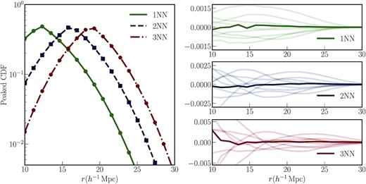
Left-hand panel: Peaked kNN-CDFs (defined in equation 18) for k ∈ {1, 2, 3}. The different lines represent the measurements of these kNN-CDFs from a random set of 10⁵ simulation particles from an N-body simulation at z = 0.5. The solid symbols represent the predictions of these kNN-CDFs computed from the smoothed matter field defined by depositing all simulation particles on a 1024³ grid, and following the procedure outlined in Section 2.1. The measurements and predictions are averaged over eight realizations at the same cosmology. The simulation volume is (1h⁻¹Gpc)³ and the total number of particles in each simulation is 512³. Right-hand panels: Darker shaded lines represent the residuals between the measurements and the predictions in the left-hand panel. The lighter shaded lines represent the variation in the measurements across realizations, i.e. sample variance. Each horizontal panel represents the residuals for a different k. Note that the y-axis stretch on each panels is different. Over the range of scales under consideration, the measurements and predictions are in very good agreement.

Open in new tab Download slide

Next, we turn to the calculations for predicting the joint CDFs. For the kNN-CDF measurements, we simply choose two disjoint subsets of 10⁵ simulation particles from the set of all simulation particles. We then compute CDF_{1, 1} using the process outlined in Banerjee & Abel (2021b). To make predictions for CDF_{1, 1} from the underlying matter field, we use the fact that this situation corresponds to setting λ_{1, i} = λ_{2, i} =λ_i in equation (14), i.e. the two underlying fields are completely correlated or identical. In terms of the smoothed matter overdensity field at scale r, equation (14) can be rewritten as

$$\begin{eqnarray} {\rm CDF}_{1,1}(r) &=& 1 - 2 \Big \langle \exp \left[- \bar{\lambda }\left(1+\delta _{r,i}\right)\right]\Big \rangle \\ &&+\, \Big \langle \exp \left[- 2\bar{\lambda }\left(1+\delta _{r,i}\right)\right]\Big \rangle \, . \end{eqnarray}$$

(19)

Therefore, in addition to the terms computed previously by averaging over the grid values, we also need to compute |$\left\langle \exp \left[-2\bar{\lambda }\delta _{r,i}\right]\right\rangle$|⁠.

The results, once again averaged over eight realizations, are plotted in Fig. 2. The upper panel plots the PCDF – the line represents the measurement of the joint CDF_{1, 1} from the particles, while the solid points represent the predictions from the continuous matter field. The bottom panel plots the residual between the prediction and the measurement using the darker shaded line. The lighter shaded lines represent the variation of the measurement itself over the eight boxes. Once again, we find that the measurements and predictions are in good agreement over the full range of scales, well within the variation from realization to realization.

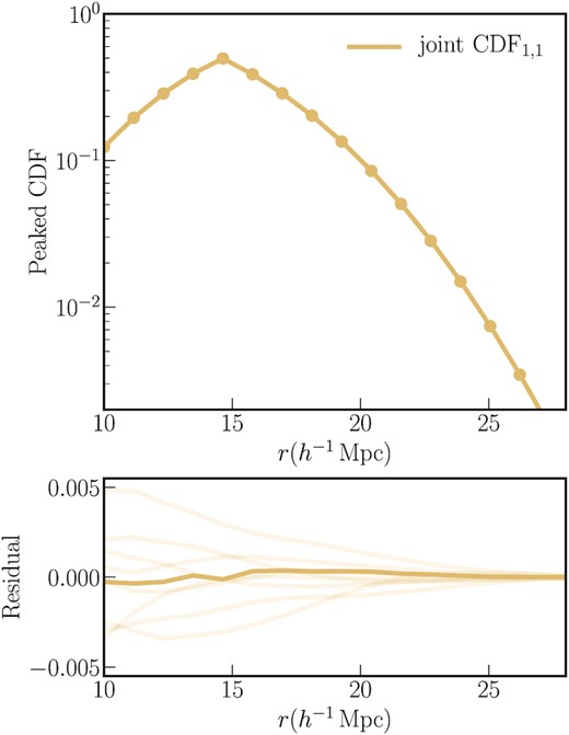
Top panel: peaked joint CDF1, 1 of two disjoint subsets of 105 particles from a 5123 particle simulation over a (1h−1Gpc)3 volume at z = 0.5. The line represents the measurement from the particles. The solid data points represent the prediction for the CDF using the statistics of the smoothed matter field on a 10243 grid, following the procedure in Section 2.1. Both the measurements and the predictions are averaged over eight realizations at the same cosmology. Bottom panel: the darker shaded line represents the residual between the measurement and the prediction in the top panel. The lighter shaded line represents the variation in the measurement of the joint CDF1, 1 from the eight different realizations compared to the mean. The joint CDF is sensitive to the cross-correlations between the two sets of tracers, and is well predicted from the statistics of the underlying matter field over the full range of scales under consideration.

Figure 2.

Top panel: peaked joint CDF_{1, 1} of two disjoint subsets of 10⁵ particles from a 512³ particle simulation over a (1h⁻¹Gpc)³ volume at z = 0.5. The line represents the measurement from the particles. The solid data points represent the prediction for the CDF using the statistics of the smoothed matter field on a 1024³ grid, following the procedure in Section 2.1. Both the measurements and the predictions are averaged over eight realizations at the same cosmology. Bottom panel: the darker shaded line represents the residual between the measurement and the prediction in the top panel. The lighter shaded line represents the variation in the measurement of the joint CDF_{1, 1} from the eight different realizations compared to the mean. The joint CDF is sensitive to the cross-correlations between the two sets of tracers, and is well predicted from the statistics of the underlying matter field over the full range of scales under consideration.

Open in new tab Download slide

Therefore, we have demonstrated that the kNN-CDFs for a set of Poisson tracers with number density |$\bar{n}$| can be accurately predicted if the underlying continuous field is known, using the process outlined in this section. Furthermore, the choice of grid size, deposition scheme and other parameter choices are good enough to produce accurate predictions over the entire range of scales of interest. This serves as a useful reference while trying to determine the range of scales over which formalism presented in Section 3 can be used to predict the kNN-CDFs of biased tracers.

3 HYBRID EFT FIELDS AND NEAREST NEIGHBOUR PREDICTIONS FOR BIASED TRACER FIELDS

In this section, we give a brief introduction to HEFT models of tracer clustering, and outline the calculational steps to predict the kNN-CDFs of a sample of tracers given the HEFT fields.

3.1 HEFT and biased tracer fields

The Lagrangian bias models that are central to HEFT assume that at the initial, Lagrangian, coordinates |${\boldsymbol q}$|⁠, the tracer density is related to the large-scale dark matter operators by a linear combination of all contributions allowed by Newtonian symmetries (Vlah et al. 2016)

$$\begin{eqnarray} \delta _X ({\boldsymbol q}) &=& F[\delta ({\boldsymbol q}), s_{ij} ({\boldsymbol q})] \\ && \approx 1 + b_1 \delta ({\boldsymbol q}) + b_2 \left(\delta ^2 ({\boldsymbol q}) - \langle \delta ^2 \rangle) \right) + \\ && b_{s^2} \left(s^2 ({\boldsymbol q}) - \langle s^2 \rangle) \right) + b_{\nabla ^2} \nabla ^2 \delta ({\boldsymbol q}) + \cdots \\ &&+\, \epsilon ({\boldsymbol q}). \end{eqnarray}$$

(20)

where we have expanded the functional F to second order. Additionally, we have defined the traceless tidal tensor field|$s_{ij} ({\boldsymbol q}) = \left(\frac{\partial _i \partial _j}{\partial ^2} - \frac{1}{3}\delta _{ij} \right) \delta ({\boldsymbol q})$|⁠. The field |$\epsilon ({\boldsymbol q})$| describes the stochastic contribution to the expansion. The stochastic term generally describes the fact the bias expansion describes a statistical relationship, and there can be deviations from this in any given realization. The stochastic fields are, by construction, uncorrelated with the bias operators |$\langle \epsilon ({\boldsymbol q}) \mathcal {O}_i \rangle = 0$|⁠. In the limit of |$\epsilon ({\boldsymbol q})$| being distributed as Gaussian white noise, its autocorrelation is constant even after advection to late-times.

The Lagrangian coordinates |${\boldsymbol q}$| are related to the current observed positions, |${\boldsymbol x}$|⁠, through a coordinate transformation

$$\begin{eqnarray} {\boldsymbol x}(a) = {\boldsymbol q}+ {\boldsymbol \Psi }({\boldsymbol q},a), \end{eqnarray}$$

(21)

where |${\boldsymbol \Psi }$| is the displacement vector that describes the motion of each Lagrangian fluid element from early times (a → 0) to a late time with scale factor a.³ In Lagrangian biasing theory (Matsubara 2008a), the late-time distribution of the tracer δ_X is then given by number conservation

$$\begin{eqnarray} 1 + \delta _X ({\boldsymbol x}) = \int {\rm d}^3 q F[\delta ({\boldsymbol q}), s_{ij}({\boldsymbol q})] \delta ^D \left({\boldsymbol x}- {\boldsymbol q}- {\boldsymbol \Psi }({\boldsymbol q}) \right) \, , \end{eqnarray}$$

(22)

where δ^D represents a Dirac delta function. Assuming a prescription for F[δ, s_ij], a model for the displacements |${\boldsymbol \Psi }$| leads to a complete model of the summary statistics of the tracer distribution δ_X. As mentioned, one can also use the |${\boldsymbol \Psi }$| from N-body simulations, as we will, leading to the classes of models called HEFT.

In practice, HEFT corresponds to assigning the simulation particles different weights based on their Lagrangian, or initial, positions in the simulation volume. As the particles evolve under their collective gravity, they carry around this ‘weight’. Note the distinction between the particle mass, which drives the gravitational evolution and the ‘weight’ which is simply carried around by the motion of the particles – changing the weights do not alter the N-body dynamics. By adjusting the values of the bias parameters, and therefore, the weights associated with the particles, the clustering of this tracer field can be adjusted to match the clustering of a target sample of haloes or galaxies. It is important to note that the bias parameters b_i considered in this paper are all scale-independent.

The tracer–tracer (P_XX(k)) and tracer–matter (P_Xm(k)) spectra, in HEFT, can then be written as sums of the cross-spectra of the advected fields in equation (20). Defining the component spectra as |$P_{ij} (k) \equiv \langle \mathcal {O}_i\mathcal {O}_j \rangle (k)$|⁠, for |$i,j \in \lbrace 1, \delta ({\boldsymbol q}), \cdots \rbrace$|⁠, we then have

$$\begin{eqnarray} P_{XX} (k) &= \sum _{i,j} b_{i}b_{j} P_{ij} (k), \end{eqnarray}$$

(23)

$$\begin{eqnarray} P_{Xm} (k) &=& P_{11}(k) + b_1 P_{1\delta }(k) + b_2 P_{1\delta ^2}(k) \\ && +\, b_{s^2} P_{1s^2}(k) + b_{\nabla ^2} P_{1\nabla ^2}(k), \end{eqnarray}$$

(24)

where in the second line above we have explicitly written out the sum. The label ‘1’ in any of the power spectra above represents the the matter density field – P₁₁(k) is the power spectrum of the matter density field. The dependence of the bias parameters in HEFT on N-point functions is analytic, however, this is not necessarily the case for other summary statistics such as kNN-CDFs.

Crucially, HEFT models allow for the construction of field-level realizations (at low redshifts) of the different operators that contribute to the bias expansion, by simply summing over the relevant weights at the low-redshift positions of the particles in the simulation. While most of the existing literature on HEFT has focused on the power spectrum as the summary statistic to quantify the clustering, the availability of the fields themselves mean that it is also possible to measure any other desired summary statistic, and assess the performance of the bias expansion beyond the traditional comparisons made at the level of the two-point correlation function. Given that kNN-CDFs measure various combinations of all connected N-point functions, their signals in HEFT are an ideal stress test of the Lagrangian bias formalism.

3.2 Computing kNN-CDFs from the HEFT fields

For a given set of bias parameters, b_i, the late-time continuous (overdensity) field |$\delta _X({\boldsymbol x})$| is defined as in equation (22). In practice, this field is defined on a grid – in this case, a 1024³ grid – by depositing the particle weights using a Cloud-in-Cell deposition scheme. To predict the values of the kNN-CDFs for tracers of this field at some radius r, we need the mean number density of the tracers |$\bar{n}$|⁠, and the δ_X field smoothed on scale r, δ_{X, r}. Given these ingredients, and the expressions in equations (15)–(17), the kNN-CDF values of the tracers can be evaluated by looping over the grid of overdensities. Any change in the values of the bias parameters b_i lead to a change in δ_X, which then propagates to a change in the kNN values when the relevant averages are preformed over the grid. To compute the predictions for the joint CDF_{1, 1} between a set of tracers of the biased HEFT field, and a set of tracers of the matter field, we use the smoothed overdensities, smoothed at scale r of both fields, δ_{X, r, i} for the HEFT field, and δ_{r, i} for the matter field:

$$\begin{eqnarray} {\rm CDF}_{1,1}(r) &=& 1 - \left\langle \exp \left[- \bar{\lambda }_X\left(1+\delta _{X,r,i}\right)\right]\right\rangle \\ &&-\, \left\langle \exp \left[- \bar{\lambda }_m\left(1+\delta _{r,i}\right)\right]\right\rangle \\ &&+ \,\left\langle \exp \left[- \bar{\lambda }_X\left(1+\delta _{X,r,i}\right) - \bar{\lambda }_m\left(1+\delta _{r,i}\right)\right]\right\rangle \, , \end{eqnarray}$$

(25)

where |$\bar{\lambda }_X = 4/3\pi r^3 \bar{n}_h$|⁠, |$\bar{\lambda }_m = 4/3\pi r^3 \bar{n}$|⁠, and |$\bar{n}_h$| and |$\bar{n}$| are the mean number density of tracers of the HEFT field and the matter field respectively. As before, the averages represent averaging these expressions over every point on the grid, labelled by the index i.

We note here that in our calculations, we assume |$\epsilon ({\boldsymbol q})$| is normally distributed with mean 0. We also assume that it is not spatially correlated, i.e. the value of |$\epsilon ({\boldsymbol q})$| at each location on the initial grid can be drawn independently from the values at other grid points. Note that, unlike the two-point correlation functions which are sensitive only to the variance of |$\epsilon ({\boldsymbol q})$|⁠, the various kNN-CDFs are formally sensitive to different moments of the distribution of |$\epsilon ({\boldsymbol q})$|⁠. However, as shown in Section 4.4, we find that for the halo samples considered in this paper, the effect of the |$\epsilon ({\boldsymbol q})$| term on the fit is negligible. Therefore, in this paper, we stick to the assumptions of Gaussianity and lack of spatial correlations stated above, and leave the investigation of the effects of loosening these assumptions to a later study. The statement that the effect of |$\epsilon ({\boldsymbol q})$| is negligible in this case is not to be conflated with the statement that we disregard shot-noise when treating the kNN-CDFs.

4 MATCHING NEAREST NEIGHBOUR CLUSTERING FOR A HALO SAMPLE

In this section, we present the results of fitting the kNN-CDFs of a set of simulation haloes using the HEFT formalism presented in Section 3. We compare the best-fitting values of b_i for the two-point functions, and the kNN-CDFs, and show that over a set of scales, both sets of summary statistics can be fit with the same values of b_i.

4.1 Defining the halo sample

For the analysis presented in this section, we once again use eight realizations from the fiducial cosmology of the Quijote simulation suite. We consider the snapshots at z = 0.5 for our calculations, since this is a typical redshift that will be probed by various current and upcoming optical surveys. The haloes are identified from the simulation particles using an FoF (Friends-of-Friends) halo finder. Since the number density |$\bar{n}$| needs to be kept constant between the measurements and predictions, we choose 10⁵ haloes from each simulation in the following way: we mass order the haloes in the halo catalogue, and throw out the most massive 10⁵ haloes and consider the mass range defined by the next 10⁵ entries. This is done to remove the very massive haloes whose clustering is not well captured by second-order HEFT down to the scales of interest. We include all haloes in the box that fall within this mass range. Since the FoF masses are discrete (in units of the particle mass), this produces a catalogue with slightly more than 10⁵ haloes. Depending on the way the halo catalogue is written out, especially when the halo list is ordered by coordinates, not performing this step could artificially distort the distribution of haloes and this distortion is propagated into the catalogue’s summary statistics. Finally, we select 10⁵ haloes at random from this catalogue to ensure a fixed number density across boxes. The haloes that make the final catalogue fall in the mass range (10^13.26−10^13.5M_⊙ h^–1) whose clustering is well described by HEFT for k ≲ 0.6h Mpc⁻¹ (see Modi et al. 2020). We will, therefore, concentrate on scales k ≲ 0.6hMpc⁻¹ or r ≳ 10h⁻¹Mpc in the rest of the paper.

We compute the kNN-CDFs for this halo sample by placing query points on a 512³ grid, similar to the measurement done in Section 2.1. To compute the joint kNN-CDF between the halo sample and the underlying matter field, which captures the cross-correlations of the two fields, we choose a random subset of 10⁵ particles from the full set of simulation particles, as representative tracers of the matter field. Our specific choice sets the number density of the haloes and the matter tracers to be the same, but this is not necessary. In order to compute the relevant tracer fields at z = 0.5, the linear fields (at z_ini = 127) relevant for the bias operators in Section 3.1 are first computed using a modified version of the 2LPT⁴ software. The bias operator fields are constructed and advected to z = 0.5 using the Anzu-fields⁵ package and the simulations’s particle positions and noiseless linear density field as input.

4.2 Using best-fitting bias values from two-point clustering

We start by fitting the autocorrelation power spectrum P_hh, and the halo-matter cross-correlation spectrum P_hm for the halo sampled defined above, using the procedure described in detail in Kokron et al. (2021). We use k_max = 0.6h Mpc⁻¹ while performing the fit, to obtain the bias parameters b_i. In Appendix A, we report the effect of how b_i obtained from changing k_max affect the kNN-CDFs. We also note that, given the treatment of the shot noise term in Kokron et al. (2021), the variance of |$\epsilon ({\boldsymbol q})$| is not determined separately from Poisson (or sampling) shot noise, and we set it to 0 in this subsection. This yields a set of bias values b_i, with which we construct the kNN-CDF predictions as outlined in Section 3.2. These predictions are compared to the actual measurements in Fig. 3. Each panel in the figure shows results for different kNN distributions – k ∈ 1, 2, 3 for the halo sample, and the joint CDF_{1, 1} between the halo sample and tracers of the matter density field. The darker solid line in each panel represents the kNN measurements. The solid circular points represent the predictions for each of the kNN-CDFs from the HEFT tracer field using the values b_i obtained from the best fitting of the auto power and cross-power spectra. To emphasize the point that the late time tracer fields are generated from the same set of particles as the matter density field, but with different weights, we also plot the kNN measurements on particles (i.e. the same ones presented in Figs 1 and 2) using the lighter dashed line in each panel, and the predictions from the matter using the square symbols.

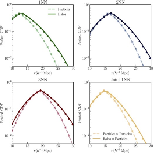
The solid lines in each panel represent the peaked CDF measurements at z = 0.5 of various kNN distributions of the sample of 105 haloes, within the mass range (1013.26−1013.5 M⊙ h–1), over a volume of (1h−1Gpc)3 defined in Section 4.1. The bottom right-hand panel shows the measurement of the joint CDF1, 1 between the halo sample and a random subset of 105 simulation particles. The circular data points represent the prediction for the different kNN-CDFs from the smoothed tracer field (Section 3.2) defined by the best-fitting values from the two-point functions of this halo sample. For contrast, the dashed lines represent the kNN measurements for 105 simulation particles instead of haloes, while the solid squares represent the predictions for these kNN-CDFs using the smoothed matter field, instead of the smoothed tracer field. All measurements and predictions are averaged over eight realizations at the same cosmology. The statistics of the smoothed tracer field are able to capture the main features of the kNN-CDFs of the haloes, even though the bias values were optimized to match the two-point clustering only.

Figure 3.

The solid lines in each panel represent the peaked CDF measurements at z = 0.5 of various kNN distributions of the sample of 10⁵ haloes, within the mass range (10^13.26−10^13.5M_⊙ h^–1), over a volume of (1h⁻¹Gpc)³ defined in Section 4.1. The bottom right-hand panel shows the measurement of the joint CDF_{1, 1} between the halo sample and a random subset of 10⁵ simulation particles. The circular data points represent the prediction for the different kNN-CDFs from the smoothed tracer field (Section 3.2) defined by the best-fitting values from the two-point functions of this halo sample. For contrast, the dashed lines represent the kNN measurements for 10⁵ simulation particles instead of haloes, while the solid squares represent the predictions for these kNN-CDFs using the smoothed matter field, instead of the smoothed tracer field. All measurements and predictions are averaged over eight realizations at the same cosmology. The statistics of the smoothed tracer field are able to capture the main features of the kNN-CDFs of the haloes, even though the bias values were optimized to match the two-point clustering only.

Open in new tab Download slide

As can be seen clearly, the kNN-CDF measurements of the particles and the haloes are clearly different, evidenced by the difference between the solid and dashed lines in each panel. However, very importantly, the change from the square data points – computed from the matter density field deposited by the particles – to the circular data points show that predictions for the kNN distributions of the haloes computed from the HEFT tracer fields capture most of this change over the range of scales of interest. This is true even though the values of bias parameters were determined using the power spectra, while the kNN-CDFs are sensitive to integrals of all connected N-point functions of the tracer fields. Further, the bottom right-hand panel shows that the same general agreement is also seen for the joint CDF_{1, 1} between the haloes and particles. This particular measurement is sensitive not only to all higher order N-point functions of the halo sample, but also to higher order N-point functions of the matter field, as well as all possible N-point functions that can be defined in terms of various combinations of the two fields (Banerjee & Abel 2021b). Therefore, the HEFT formalism can potentially fit not just the two-point clustering of the halo sample in terms of the two-point functions of various advected Lagrangian fields, but also various higher order statistics. We explore this in more detail below.

4.3 Response to changes in bias values

We now investigate the response of the kNN distributions under consideration to changes in the values of the bias parameters around those obtained by fitting the two-point functions in Section 4.2. To do this, we change the bias values, one at a time, by |$5\,{{\rm per\,cent}}$| (⁠|$b_{i}^+$| and |$b_{i}^-$|⁠) around the best-fitting values, |$b_i^{\rm fid}$|⁠. We recompute the predictions for the various kNN-CDFs with this new set of b_i, and express the change in terms of the logarithmic derivative of the quantities:

$$\begin{eqnarray} \frac{\partial \log \mathcal {O}}{\partial b_i} \simeq \frac{1}{\mathcal {O} \left(b_i^{\rm fid}\right)}\frac{\mathcal {O}\left(b_i^+\right) - \mathcal {O}\left(b_i^-\right)}{b_i^+ - b_i^-} \, , \end{eqnarray}$$

(26)

where |$\mathcal {O}$| represents the various kNN-CDFs under consideration. Since we assumed |$\langle \epsilon ({\boldsymbol q})^2\rangle = 0$| in the previous subsection, this parameter needs to be treated differently here. In this case, we use one-sided finite difference for positive values of |$\langle \epsilon ({\boldsymbol q})^2\rangle$| instead of a centred finite difference to approximate the derivative. To compute the one-sided finite difference, we evaluate the tracer fields and kNN predictions for |$\sqrt{\langle \epsilon ({\boldsymbol q})^2\rangle } \in {0,0.1,0.2}$|⁠.

The results are presented in Fig. 4. Each panel represents the change in the logarithmic derivative of a different kNN-CDF. The different lines on each panel represent the response of that particular kNN-CDF prediction to a change in each of the bias parameters. Note that the logarithmic derivatives with respect to different bias parameters have been multiplied by different factors to make the changes visible on the same plot. As with the two-point functions, the kNN-CDF predictions are most sensitive to the linear bias value b₁, but all the bias parameters produce measurable changes on the different kNN distributions. Further, the same bias parameter, e.g. b₁, affects the different kNN distributions at different levels. This suggests that combining different kNN measurements in an analysis can help break degeneracies. We will explore this further in Section 5.

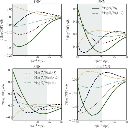
$Logarithmic derivatives (around the best-fitting values discussed in Section 4.2) of different kNN-CDFs with respect to the second-order Lagrangian bias parameters $b_1, b_2, b_{s^2}$, and $b_{\nabla ^2}$. Each panel shows the response of a given kNN distribution, while lines of the same colour represent the same bias parameter across the different panels. The grey shaded regions in each panel represent the scales where the HEFT predictions cannot accurately model the measurements, as discussed in Section 4.4. Similar to the two-point function, the predictions are most sensitive to changes in b1.$

Figure 4.

Logarithmic derivatives (around the best-fitting values discussed in Section 4.2) of different kNN-CDFs with respect to the second-order Lagrangian bias parameters |$b_1, b_2, b_{s^2}$|⁠, and |$b_{\nabla ^2}$|⁠. Each panel shows the response of a given kNN distribution, while lines of the same colour represent the same bias parameter across the different panels. The grey shaded regions in each panel represent the scales where the HEFT predictions cannot accurately model the measurements, as discussed in Section 4.4. Similar to the two-point function, the predictions are most sensitive to changes in b₁.

Open in new tab Download slide

4.4 Best-fitting to kNN-CDFs and range of scales of validity

Having established that changes in the bias parameters produce distinctive responses in the predictions for the kNN-CDFs for tracer of the HEFT fields, we now present the results of optimizing the bias parameters to fit the kNN-CDFs of the halo samples from the simulations. For the purposes of this first study, the bias parameters are changed by hand until the residuals discussed below are within the error bars. The results are presented in Fig. 5. We plot the residuals between the measurements of the halo kNN-CDFs and the predictions for the same from the smoothed tracers fields. The dashed lines represent the residuals for the case when the best-fitting values from fitting the power spectra were used. The solid lines represent the residuals for the best fit to the actual kNN-CDF measurements. Each of the lines is produced by averaging over eight realizations. The coloured bands around 0 represent the variance of the kNN-CDF measurements themselves from 100 realizations at the same cosmology. We find that the best-fitting bias parameters for the (auto and cross) power spectra of the halo sample are not optimal fits for the kNN-CDFs of the halo sample. A better fit can be produced by changing the values of the bias parameters, as seen by the solid lines in Fig. 5. Even in this case, however, depending on the kNN distribution under consideration, the prediction from the HEFT fields is a good fit, as defined by the spread of measurements across different realizations, to the halo measurements over a certain range of scales. The agreement persists down to the smallest scales for the 1NN distribution (top left-hand panel), ∼16 h⁻¹ Mpc. For the 2NN distribution of the haloes (top right-hand panel), and the joint distribution of haloes and tracers of the matter field (bottom right-hand panel), the best-fit is a good match to the measurements down to ∼20 h⁻¹Mpc. For the 3NN distribution (bottom left-hand panel), the HEFT predictions are only a good fit at ≳ 24 h⁻¹Mpc. These cutoff scales, below which the HEFT predictions do accurately model the kNN measurements are indicated by the shaded grey regions in each panel of Fig. 5. For context, the power spectra, P_hh and P_hm, are well-fit by the HEFT prescription down to |$k_{\rm max} \sim 0.6 \, h{\rm Mpc}^{-1}$| or r ∼ 10.5h⁻¹Mpc. Since the higher kNN distributions are more sensitive to the higher density regions (see equations 15–17 for reference), these finding suggests that the HEFT fields do not fully replicate the clustering of haloes in the highest density environments to this order in the Lagrangian bias expansion. On the other hand, for the 1NN-CDF is dominated by the distribution of the lowest density regions in the simulation, and the HEFT prescription does a good job of capturing the distribution down to scales closer to that for the power spectra. We note here that the kNN best-fits are consistent with |$\sqrt{\langle \epsilon ({\boldsymbol q})^2\rangle } =0$|⁠.

Figure 5.

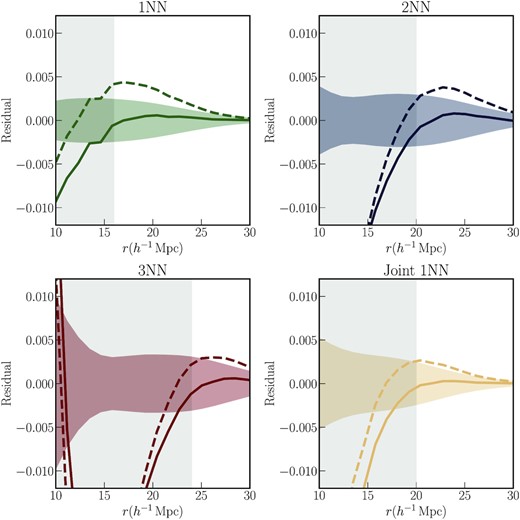
Residuals between the kNN-CDF measurements of the halo sample from Section 4.1 and the predictions for the same generated using the smoothed HEFT fields. Each panel represents a different kNN distribution. The dashed lines represent the residuals in the case when the tracer fields were generated using the best-fitting values from fitting the halo auto and cross power spectra. The solid lines represent the residuals when the bias values are optimized to fit the kNN distributions of the haloes. All measurements and predictions are averaged over eight realizations. The shaded regions around 0 represent the scatter in the halo kNN measurements from 100 realizations. The grey shaded regions in each panel represent the scales where the HEFT predictions cannot accurately model the measurements. The solid lines show that there exist combinations of the bias parameters that produce a good fit to the halo kNN-CDFs over certain range of scales. The agreement extends down to the smallest scales for the 1NN distribution ∼16 h⁻¹Mpc. See Fig. 6 for the residuals with respect the power spectra measurements for the same set of bias parameters.

Open in new tab Download slide

In order for the HEFT model to model both the power spectra measurement, and the kNN measurements of a given tracer sample, it is crucial that the same set of bias values produce good fits for both sets of measurements. Therefore, we compute the predictions for the auto and cross power spectra given the bias values obtained from the kNN distribution fitting, and compare it to the measurements. In Fig. 6, we plot the residuals from this process using the solid lines. The dotted lines represent the residuals from the best-fit to the two-point measurements themselves (as used in Section 4.2). The left-hand panel is for the auto power spectrum (P_hh) measurements, while the right-hand panel is for the halo-matter cross-spectrum (P_hm) measurements. The shaded region represents the spread in measurements from 100 realizations. As can be seen, the solid lines are still a good fit to the measurements, given the error bars. Therefore, in the presence of these scale cuts, the same number of bias parameters, and equally importantly, the same values of these bias parameters in the HEFT framework can be used to model both the auto and cross power spectra of a set of tracers, as well as the kNN distributions of the same set of tracers.

Figure 6.

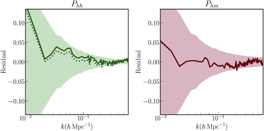
Residuals between the power spectra measurements of the halo sample from Section 4.1 and the predictions for the same generated using the HEFT fields. The left-hand panel represents measurements and predictions of the halo auto spectrum, P_hh(k). The right-hand panel represents measurements and predictions of the halo-matter cross power spectrum P_hm(k). The dotted lines represent the residuals in the case when the tracer fields were generated using the best-fitting values from the halo auto and cross power spectra. The solid lines represent the residuals when the bias values are optimized to fit the kNN distributions of the haloes, the same as the solid line in Fig. 5. All measurements and predictions are averaged over eight realizations. The shaded regions represent the scatter in the power spectra measurements from 100 realizations. The difference between the two sets of curves is more pronounced in the left-hand panel. Given the measurement uncertainties, the best-fitting bias values obtained by fitting the kNN distributions are also provide a good fit to the power spectra measurements of the same halo sample.

Open in new tab Download slide

It is interesting to note that the change between the two-point best fit and the kNN best fit – i.e. the change from the dashed lines to the solid lines in Fig. 5 – is produced primarily by a change in the value of |$b_{s^2}$|⁠. The value of |$b_{s^2}$| changes by 13 per cent between the two. Kokron et al. (2021) found that the tracer–tracer and tracer–matter spectra are least sensitive to varying |$b_{s^2}$|⁠. It is therefore the hardest to constrain with only these statistics, as evidenced by the simulated likelihood analyses carried out therein. This can be understood, partially, by noting that the halo–matter spectrum is only sensitive to the parameter |$b_{s^2}$| through the basis spectrum |$P_{1s^2}(k)$| (equation 24). This spectrum is orders of magnitude smaller than other basis spectra at all scales (see fig. 1 of Kokron et al. 2021).

Given the results presented above the kNN distributions appear to be much more sensitive to |$b_{s^2}$|⁠, and therefore should be able to constrain it much more strongly than P(k) measurements can. This suggests using kNN measurements can be highly complementary to the traditional P(k) or two-point measurements, and combining them can help realize the full power of the HEFT framework in extracting cosmological parameter constraints from tracers of cosmological structure. We explore this aspect further in Section 5.

5 FISHER ESTIMATES FOR PARAMETER CONSTRAINTS

In this section, we demonstrate that using kNN-CDF measurements in addition to the traditional two-point function (or P(k)) measurements can improve constraints on both the HEFT model parameters, as well as the underlying cosmological parameters. To do this, we use the Fisher matrix formalism. The entries of the Fisher matrix (⁠|$\boldsymbol{F}$|⁠) are defined as

$$\begin{eqnarray} \boldsymbol{F}_{\alpha \beta } = \sum _{i,j}\frac{\partial D_i}{\partial p_\alpha } \bigg [\boldsymbol{C}^{-1}\bigg ]_{ij} \frac{\partial D_j}{\partial p_\beta }\, , \end{eqnarray}$$

(27)

where D_i represent the entries of the data vector under consideration (e.g. P(k) values), p_α represent the parameters we are looking to constrain using the data vector. |$\boldsymbol{C}$| represents the covariance matrix of the data vector at the fiducial set of parameters. We will consider two data vectors: the first is a data vector with the auto and cross power spectra of the HEFT fields with |$k_{\rm max} = 0.6 \, h{\rm Mpc}^{-1}$|⁠. The second data vector is constructed by adding the kNN-CDFs of the HEFT fields to the first data vector. We note that we use the kNN-CDFs only on the scales where the HEFT fields provided a good fit to the halo sample in Section 4.4 – 16h⁻¹Mpc for the 1NN-CDF, and 20h⁻¹Mpc for the 2NN-CDF and joint CDF_{1, 1} between the HEFT field and the matter field. We discard the measurements on smaller scales, indicated by the grey shaded regions in Fig. 5. Since the range over which it is well modelled by HEFT is small, we do not use the 3NN-CDF in this analysis. We have shown in Section 4.4 that a single set of bias values can fit both the two-point clustering and the kNN distributions of a tracer sample. Therefore, in this illustrative example, the HEFT fields and the clustering predictions are generated using the best-fitting values used in Section 4.2 for the halo sample identified in Section 4.1. In Appendix C, we repeat the analysis for fiducial bias values that are representative of a different sample of tracers. The full set of parameters we use in this analysis are two cosmological parameters – σ₈ and Ω_m, and the set of HEFT bias parameters – b₁, b₂, |$b_{s^2}$|⁠, and |$b_{\nabla ^2}$|⁠. Note that in addition to these parameters, the P(k) fit also uses a term controlling the shot-noise amplitude.

To generate measurements over different realizations, we use the Quijote simulation suite – we estimate the covariance matrices for each data vector using 1000 realizations of the fiducial cosmology in the Quijote suite. Specifically, to ensure that our covariance matrix properly captures the cross-correlations between the power spectra and the kNN-CDFs, for each box in the covariance suite we generate the HEFT field |$\delta _{h}({\boldsymbol x})$| from the fiducial bias values adopted in the forecast. The whole data vector is measured over this HEFT field. To compute the derivatives of the {P_hh, P_hm}, however, we use equations (23) and (24) and the measured basis spectra P_XY for each box. Since a finite number of realizations are used to estimate the covariance matrix, we use the appropriate Hartlap factor (Hartlap, Simon & Schneider 2007) to correct for this. The cosmological derivatives, i.e. with respect to σ₈ and Ω_m are computed using 100 realizations of the |$\sigma _8 ^\pm$| and |$\Omega _{\rm m} ^\pm$| cosmologies from the same suite (Villaescusa-Navarro et al. 2020). The derivatives with respect to the bias parameters are computed using 100 realizations of the fiducial cosmology, but by changing the bias values by 5 per cent around the fiducial values. The 1σ constraints on the parameters, labelled by α, are obtained from the Fisher matrix as

$$\begin{eqnarray} \sigma _\alpha = \sqrt{\big ({\boldsymbol F}^{-1}\big)_{\alpha \alpha }}\, . \end{eqnarray}$$

(28)

It should be noted that the standard Fisher error on parameter α represents the uncertainty after having marginalized over the other model parameters.

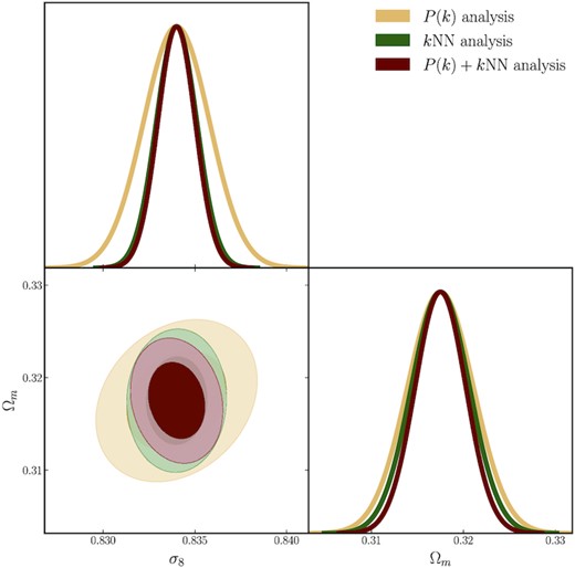
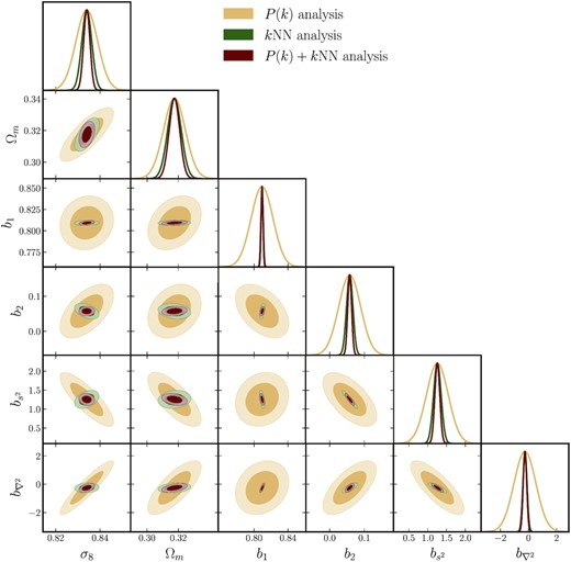
The results of the analysis are presented in Fig. 7. The 1σ constraints on individual parameters are summarized in Table 1.The yellow contours and yellow standard Fisher errors in Fig. 7 represent the results from the P(k) Fisher analysis. The maroon contours and standard Fisher errors in Fig. 7 represent the results from the combined P(k) and kNN-CDF analysis. We also plot the results from the kNN-only analysis using the green contours and standard Fisher errors. We find that, for this halo sample, the constraints on σ₈ improve by roughly a factor of 3 when the kNN-CDF measurements are added to the P(k) measurements (maroon curves), while for Ω_m, the improvement is somewhat smaller, |$\sim 60{{\rm per\,cent}}$|⁠. This improvement in the cosmological parameter constraints can be summarized in terms of the Figure of Merit (FoM) in the Ω_m−σ₈ plane, that is, the inverse of the area of the ellipse in Fig. 7. The FoM increases by a factor of 3.1 when kNN measurements are added to the P(k) measurements. By comparing the maroon and the green contours, it is clear that much of the gains are driven by the kNN distributions alone. For the bias parameters also, the standard Fisher errors are drastically reduced, for b₁ and |$b_{s^2}$| in particular, when the kNN information is folded in. This is consistent with our finding in Section 4.4 where a change in |$b_{s^2}$| was the primary difference between the P(k) best-fit and the kNN best fit. It is also worth noting that once again, the kNN measurements (green curves) drive most of the gain, even more so than for the cosmological parameters. Since the bias parameters are chosen to be scale-independent, the kNN measurements on relatively small scales are able to constrain the parameters precisely, and the P(k) measurements do not add to the constraints. The cosmological parameters, on the other hand, produce unique changes on large scales that are not included in the kNN measurements, but are used in the P(k) measurements. Therefore, combining the P(k) and kNN measurements results in tighter constraints for the cosmological parameters than either set of measurements alone. The reduction in the uncertainties in the bias parameters, when kNN measurements are included, is exactly what drives the improvement in the cosmological constraints compared to the P(k)-only analysis. We explore this point further in Appendix B, where we hold the bias parameters fixed, and compare the improvements on the cosmological parameters only. The cosmological and bias parameters can have somewhat degenerate effects on the two-point clustering, but by combining with the kNN measurements, these degeneracies can be broken. We therefore conclude that there are potentially large gains to be made in terms of parameter constraints using the HEFT formalism when the kNN statistics are included to capture the clustering of tracers in addition to the two-point clustering.

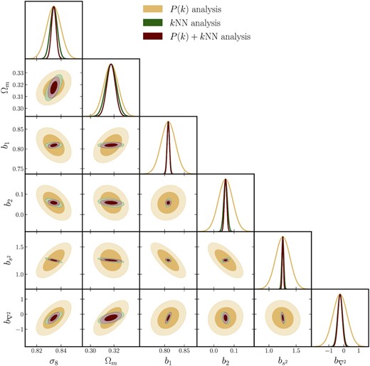
$Results of the Fisher analysis presented in Section 5. The yellow contours and standard Fisher errors represent the results when only the auto and cross power spectra of the HEFT fields are considered (up to $k_{\rm max} = 0.6 \, h{\rm Mpc}^{-1}$). The green contours represent the standard Fisher errors from the analysis of the kNN measurements, over the range of scales discussed in the text. The marooon contours and standard Fisher errors represent the results of combining the P(k) and kNN measurements. All forecasts assume the fiducial Quijote volume of V = 1(h−1Gpc)3. For this sample, adding in the kNN measurements improves the constraints on σ8 by a factor of 3, and that on Ωm by $\sim 60\,{{\rm per\,cent}}$ over the P(k)-only analysis. The HEFT bias parameters are also better constrained when kNN measurements are included.$

Figure 7.

Results of the Fisher analysis presented in Section 5. The yellow contours and standard Fisher errors represent the results when only the auto and cross power spectra of the HEFT fields are considered (up to |$k_{\rm max} = 0.6 \, h{\rm Mpc}^{-1}$|⁠). The green contours represent the standard Fisher errors from the analysis of the kNN measurements, over the range of scales discussed in the text. The marooon contours and standard Fisher errors represent the results of combining the P(k) and kNN measurements. All forecasts assume the fiducial Quijote volume of V = 1(h⁻¹Gpc)³. For this sample, adding in the kNN measurements improves the constraints on σ₈ by a factor of 3, and that on Ω_m by |$\sim 60\,{{\rm per\,cent}}$| over the P(k)-only analysis. The HEFT bias parameters are also better constrained when kNN measurements are included.

Open in new tab Download slide

Table 1.

Open in new tab

1σ constraints on cosmological and HEFT parameters, from the P(k)-only, kNN-only, and P(k) + kNN Fisher analysis discussed in Section 5.

Parameter	σ_P(k)	σ_kNN	σ_{P(k) + kNN}
σ₈	0.0058	0.0030	0.0019
Ω_m	0.0061	0.0046	0.0036
b₁	0.0182	0.0032	0.0029
b₂	0.0353	0.0091	0.0060
\|$b_{s^2}$\|	0.1314	0.0188	0.0116
\|$b_{\nabla ^2}$\|	0.4787	0.1677	0.1460

Parameter	σ_P(k)	σ_kNN	σ_{P(k) + kNN}
σ₈	0.0058	0.0030	0.0019
Ω_m	0.0061	0.0046	0.0036
b₁	0.0182	0.0032	0.0029
b₂	0.0353	0.0091	0.0060
\|$b_{s^2}$\|	0.1314	0.0188	0.0116
\|$b_{\nabla ^2}$\|	0.4787	0.1677	0.1460

Table 1.

Open in new tab

1σ constraints on cosmological and HEFT parameters, from the P(k)-only, kNN-only, and P(k) + kNN Fisher analysis discussed in Section 5.

Parameter	σ_P(k)	σ_kNN	σ_{P(k) + kNN}
σ₈	0.0058	0.0030	0.0019
Ω_m	0.0061	0.0046	0.0036
b₁	0.0182	0.0032	0.0029
b₂	0.0353	0.0091	0.0060
\|$b_{s^2}$\|	0.1314	0.0188	0.0116
\|$b_{\nabla ^2}$\|	0.4787	0.1677	0.1460

Parameter	σ_P(k)	σ_kNN	σ_{P(k) + kNN}
σ₈	0.0058	0.0030	0.0019
Ω_m	0.0061	0.0046	0.0036
b₁	0.0182	0.0032	0.0029
b₂	0.0353	0.0091	0.0060
\|$b_{s^2}$\|	0.1314	0.0188	0.0116
\|$b_{\nabla ^2}$\|	0.4787	0.1677	0.1460

While we have demonstrated this using a specific halo sample here, we show in Appendix C that similar statistical gains from kNN measurements are expected to hold for another tracer sample relevant to various cosmological surveys – the redMaGiC galaxy sample (Elvin-Poole et al. 2018), provided that the modelling assumptions in this study extend to such a sample. Note that just the fact the constraints on all parameters improve when kNN measurements are considered in addition to the P(k) measurements is not surprising in itself, since the addition of any statistics sensitive to the model parameters will improve the final constraints. However, it is worth pointing out again that the large improvements demonstrated above are possible because the kNN modelling does not require any additional model parameters compared to those needed to model the P(k) measurements of the tracers. Indeed, this is one of the most important and useful conclusions from this study.

6 SUMMARY AND DISCUSSION

In this paper, we have demonstrated how the HEFT formalism (Modi et al. 2020; Kokron et al. 2021; Zennaro et al. 2021) can be used to model the k-nearest neighbour distributions (Banerjee & Abel 2021a) of a set of biased tracers of the cosmological matter field over a range of scales in real space. To do so, we have developed the formalism to predict the kNN-CDFs of a set of Poisson tracers of a continuous field in terms of various averages of the underlying field smoothed on various scales. We have demonstrated the power of this formalism by computing the predictions for the kNN-CDF of a random subset of simulation particles at z = 0.5 in terms of matter density field at that redshift. We then use the same setup to match the kNN-CDF measurements of a sample of haloes from the Quijote simulations using the HEFT component fields and a set of values for the bias parameters. We show that even when the bias parameters are determined by fitting the auto and cross (with matter) power spectra of the haloes, i.e. two-point functions, the kNN-CDF predictions from the resultant weighted HEFT fields provide a good approximation of the actual kNN-CDF measurements from the halo sample. It is worth reiterating that the kNN-CDF predictions depend on integrals of all connected N-point functions of the HEFT fields. We have explored how the kNN-CDF predictions from the HEFT fields change in response to changes in the values of the bias parameters, and found that each bias parameter produces a unique response, especially when multiple nearest neighbour distributions are considered together. Crucially, we have then demonstrated that there exist a set of bias values, and by extension, a set of weighted HEFT fields, which can match both the two-point clustering and the kNN clustering of the halo sample, over a range of scales, with the 1NN distribution most accurately predicted down to smaller scales. Finally, using a Fisher analysis, we show that including the kNN measurements, in addition to the two-point measurements, can lead to much improved constraints on cosmological parameters within the HEFT framework. For σ₈ in particular, this improvement is roughly a factor of 3. This paper, therefore, outlines a way of combining the HEFT modelling of biased tracers with the statistical power of the kNN formalism that can potentially extract much more information about the cosmological parameters of interest from quasi-linear scales probed by various surveys. We discuss some features of this study in further detail below.

While the kNN measurements are very sensitive to clustering information on scales below ∼30 h⁻¹ Mpc for the number density of tracers considered in this paper, these measurements do not fully capture the information on larger scales where the CDFs all tend to 1. Considering the kNN measurements by themselves would, for example, miss out on the information from the baryon acoustic oscillation (BAO) scales (∼100 h⁻¹Mpc). Therefore, combining the large-scale clustering information from the two-point function measurements with kNN measurements, which characterize the small-scale clustering accurately, represents an optimal data vector to measure clustering on all scales. Further, since the bias parameters affect the two-point function and the kNN prediction in HEFT in different ways, the combination of these quantities also helps break various degeneracies.

The original formulation of the HEFT framework in Modi et al. (2020) increased the range of scales over which the same set of Lagrangian bias parameters can be used to model the clustering of tracers compared to perturbation theory approaches, focusing on power spectra measurements to determine the range of scales. The model is able to match not only the auto power spectra of tracers, but also the tracer–matter cross-spectrum. However, since the model explicitly uses the gravitational evolution of a N-body simulation particles, a characteristic feature of this model is that its primary output is a late-time non-linear field rather than any particular late-time summary statistic. Therefore, it is also possible to compute and compare any higher order statistics between the HEFT predictions and a set of tracers. This is the first study which does so, by considering the kNN statistics of the tracer samples and the HEFT fields, which depends on integrals of all connected N-point functions of the fields. The fact that the kNN statistics of the tracer sample can be modelled by the HEFT framework – without expanding the number of free parameters needed – over a range of scales, indicates that the HEFT formalism indeed works at the field level. This is further supported by the fact that the HEFT predictions also match the joint CDF between the tracers and matter. This particular CDF is sensitive to integrals of all possible N-point correlation functions between the tracer field and the underlying matter field, and can only be modelled correctly when both fields are evolved correctly. This suggests that while predicting kNN distributions, as was done in this paper, is particularly simple, the HEFT framework can also be applied to other higher order summary statistics that have been explored in the literature.

As shown in Section 4.4, the range of scales over which the HEFT framework is able to fit the kNN distributions of tracers is not the same as the set of scales over which it provides a good fit to the power spectra, which are well-fitting down to smaller scales. For the 1NN, the smallest scale that is accurately modelled, r ≥ 16h⁻¹Mpc, is roughly comparable to that for the power spectrum. For higher kNN distributions, and for the joint distributions between the tracers and the matter field, the HEFT framework is only accurate at larger scales of r ≥ 20h⁻¹Mpc. Given the statistical power of the kNN statistics, it will be interesting to explore if the modelling, especially for the higher and joint NN distributions, can be extended to smaller scales. One possibility is to include higher order bias terms – currently terms up second order are included. Since the N-body dynamics themselves do not change with the inclusion of these terms, they simply represent more degrees of freedom in how the particle weights that make up the final HEFT fields can be distributed. However, it should be pointed that the number of terms allowed by symmetries keep increasing at higher orders, and thereby introducing many additional free parameters which need to be constrained by the data, in addition to the cosmological parameters of interest (Abidi & Baldauf 2018; Lazeyras & Schmidt 2018). Therefore, it needs to be investigated whether the gain in statistical power by modelling the kNN distribution from HEFT down to smaller scales is sufficient to offset the increase in the number of model parameters. For theoretical studies of higher order biasing in HEFT, though, the statistical power of the nearest neighbour framework, along with the ease of calculation, should provide the right framework to isolate and understand the effects of these higher order terms on late-time clustering of biased tracers.

The first step towards performing full cosmological analyses that harness the power of adding kNN measurements within the HEFT framework will be to predict these statistics as a joint function of the cosmological parameters and the bias parameters. Given that full N-body simulations are an essential component of the HEFT prediction, the emulator approach, which is increasingly being applied in the cosmological context, is best suited to this. Kokron et al. (2021), Zennaro et al. (2021), and Hadzhiyska et al. (2021) have already the applied emulator approach to predicting the auto and cross-power spectra of tracers as a function of cosmology and HEFT bias parameters. One of the natural extensions of this paper is to build a similar framework for kNN predictions, and will be explored in a future study.

Another notable extension of this work is to further investigate the impact of the stochasticity, |$\epsilon ({\boldsymbol q})$|⁠, on our predictions. While we have found it sufficient to treat the field as Gaussian distributed with mean zero, some other recent studies (see e.g. Friedrich et al. 2021) report the need for a non-Poisson stochastic term in the modelling of a related statistic – the PDF of projected galaxy counts. However, a direct comparison between results is difficult to make for multiple reasons. Friedrich et al. (2021) concerns itself with a population of galaxies in projected space whereas we limit ourselves to a different halo sample in real space. Secondly, Friedrich et al. (2021) uses a cylindrical collapse approach to the evolution of the underlying field, whereas this study makes use of N-body simulations for the same. Finally, the bias models themselves are somewhat different, since Friedrich et al. (2021) restrict themselves to terms proportional to b₁ and b₂. Indeed, it is known that at the two-point function level (Baldauf et al. 2013; Ginzburg, Desjacques & Chan 2017) super-Poissonian stochasticity can arise from neglected bias operators. As we have pointed out in Fig. 5 the impact of slightly altering the tidal bias (⁠|$b_{s^2}$|⁠) in the residuals is significant, but this operator is neglected in Friedrich et al. (2021). Nevertheless, a more complete understanding and a thorough comparison of one-point PDF statistics, higher order Lagrangian bias models and stochasticity is of great interest, and we defer it for future work. In principle, if the resulting non-Poissonianity can be captured as a white noise field with a different variance than expected, our treatment of stochasticity should still be sufficient. It is also possible to augment our current model by connecting the continuous field and the tracer (halo) sample through the two-parameter functional form used in Friedrich et al. (2018, 2021), rather than the single parameter Poisson sampling.

ACKNOWLEDGEMENTS

The authors thank Andrey Kravtsov, Jessie Muir, and Risa Wechsler for helpful comments on an earlier version of this manuscript. We thank the referee for insightful comments which helped improve the paper. This work was supported by the Fermi Research Alliance, LLC under Contract No. DE-AC02-07CH11359 with the U.S. Department of Energy, the U.S. Department of Energy (DOE) Office of Science Distinguished Scientist Fellow Program, and the U.S. Department of Energy SLAC Contract No.DE-AC02-76SF00515. Some of the computing for this project was performed on the Sherlock cluster. The authors would like to thank Stanford University and the Stanford Research Computing Center for providing computational resources and support that contributed to these research results. The Pylians3⁶ and nbodykit (Hand et al. 2018) analysis libraries were used extensively in this paper. We also acknowledge the use of the GetDist⁷ (Lewis 2019) software for plotting.

DATA AVAILABILITY

The simulation data used in this paper is publicly available at https://github.com/franciscovillaescusa/Quijote-simulations. Additional data are available on reasonable request.

Footnotes

1

http://www.sdss3.org/surveys/boss.php

2

https://github.com/franciscovillaescusa/Quijote-simulations

3

We will suppress the scale factor a in subsequent equations so as to not over-load notation.

4

https://cosmo.nyu.edu/roman/2LPT/

5

https://github.com/kokron/anzu

6

https://github.com/franciscovillaescusa/Pylians3

7

https://getdist.readthedocs.io/en/latest/

8

http://www.unitsims.org/

REFERENCES

Abidi

M. M.

,

Baldauf

T.

,

2018

,

J. Cosmol. Astropart. Phys.

,

2018

,

029

10.1088/1475-7516/2018/07/029

Crossref

Search ADS

Alam

S.

et al. ,

2021

,

Phys. Rev. D

,

103

,

083533

10.1103/PhysRevD.103.083533

Crossref

Search ADS

Baldauf

T.

,

Seljak

U.

,

Smith

R. E.

,

Hamaus

N.

,

Desjacques

V.

,

2013

,

Phys. Rev. D

,

88

,

083507

10.1103/physrevd.88.083507

Crossref

Search ADS

Banerjee

A.

,

Abel

T.

,

2021a

,

MNRAS

,

500

,

5479

10.1093/mnras/staa3604

Crossref

Search ADS

Banerjee

A.

,

Abel

T.

,

2021b

,

MNRAS

,

504

,

2911

10.1093/mnras/stab961

Crossref

Search ADS

Carlson

J.

,

Reid

B.

,

White

M.

,

2012

,

MNRAS

,

429

,

1674

10.1093/mnras/sts457

Crossref

Search ADS

Chen

S.-F.

,

Lee

H.

,

Dvorkin

C.

,

2021

,

J. Cosmol. Astropart. Phys.

,

2021

,

030

10.1088/1475-7516/2021/05/030

Crossref

Search ADS

Chuang

C.-H.

et al. ,

2019

,

MNRAS

,

487

,

48

10.1093/mnras/stz1233

Crossref

Search ADS

Clampitt

J.

et al. ,

2017

,

MNRAS

,

465

,

4204

10.1093/mnras/stw2988

Crossref

Search ADS

d’Amico

G.

,

Gleyzes

J.

,

Kokron

N.

,

Markovic

K.

,

Senatore

L.

,

Zhang

P.

,

Beutler

F.

,

Gil-Marín

H.

,

2020

,

J. Cosmol. Astropart. Phys.

,

2020

,

005

10.1088/1475-7516/2020/05/005

Crossref

Search ADS

DeRose

J.

et al. ,

2019

,

The Buzzard Flock: Dark Energy Survey Synthetic Sky Catalogues

,

preprint (arXiv:1901.02401)

DES Collaboration

et al. .,

2021

,

Phys. Rev. D

,

105

,

023520

DESI Collaboration

et al. .,

2016

,

preprint (arXiv:1611.00036)

Desjacques

V.

,

Jeong

D.

,

Schmidt

F.

,

2018

,

Phys. Rep.

,

733

,

1

10.1016/j.physrep.2017.12.002

Crossref

Search ADS

Doré

O.

et al. ,

2014

,

preprint (arXiv:1412.4872)

Dore

O.

et al. ,

2019

,

BAAS

,

51

,

341

Elvin-Poole

J.

et al. ,

2018

,

Phys. Rev. D

,

98

,

042006

10.1103/PhysRevD.98.042006

Crossref

Search ADS

Friedrich

O.

et al. ,

2018

,

Phys. Rev. D

,

98

,

023508

10.1103/PhysRevD.98.023508

Crossref

Search ADS

Friedrich

O.

,

Halder

A.

,

Boyle

A.

,

Uhlemann

C.

,

Britt

D.

,

Codis

S.

,

Gruen

D.

,

Hahn

C.

,

2021

,

MNRAS

,

510

,

5069

Crossref

Search ADS

Ginzburg

D.

,

Desjacques

V.

,

Chan

K. C.

,

2017

,

Phys. Rev. D

,

96

,

083528

10.1103/physrevd.96.083528

Crossref

Search ADS

Gruen

D.

et al. ,

2015

,

MNRAS

,

455

,

3367

10.1093/mnras/stv2506

Crossref

Search ADS

Hadzhiyska

B.

,

García-García

C.

,

Alonso

D.

,

Nicola

A.

,

Slosar

A.

,

2021

,

J. Cosmol. Astropart. Phys.

,

2021

,

020

Hahn

C.

,

Villaescusa-Navarro

F.

,

2021

,

J. Cosmol. Astropart. Phys.

,

2021

,

029

10.1088/1475-7516/2021/04/029

Crossref

Search ADS

Hahn

C.

,

Villaescusa-Navarro

F.

,

Castorina

E.

,

Scoccimarro

R.

,

2020

,

J. Cosmol. Astropart. Phys.

,

2020

,

040

10.1088/1475-7516/2020/03/040

Crossref

Search ADS

Hand

N.

,

Feng

Y.

,

Beutler

F.

,

Li

Y.

,

Modi

C.

,

Seljak

U.

,

Slepian

Z.

,

2018

,

ApJ

,

156

,

160

10.3847/1538-3881/aadae0

Crossref

Search ADS

Hartlap

J.

,

Simon

P.

,

Schneider

P.

,

2007

,

A&A

,

464

,

399

10.1051/0004-6361:20066170

Crossref

Search ADS

Heitmann

K.

et al. ,

2008

,

Comput. Sci. Discovery

,

1

,

015003

10.1088/1749-4699/1/1/015003

Crossref

Search ADS

Heitmann

K.

,

Ricker

P. M.

,

Warren

M. S.

,

Habib

S.

,

2005

,

ApJS

,

160

,

28

10.1086/432646

Crossref

Search ADS

Heymans

C.

et al. ,

2021

,

A&A

,

646

,

A140

10.1051/0004-6361/202039063

Crossref

Search ADS

Hockney

R. W.

,

Eastwood

J. W.

,

1988

,

Computer Simulation Using Particles

.

Taylor and Francis, Inc

,

Boca Raton

Ivanov

M. M.

,

Simonović

M.

,

Zaldarriaga

M.

,

2020

,

J. Cosmol. Astropart. Phys.

,

2020

,

042

10.1088/1475-7516/2020/05/042

Crossref

Search ADS

Ivezić

Ž.

et al. ,

2019

,

ApJ

,

873

,

111

10.3847/1538-4357/ab042c

Crossref

Search ADS

Kokron

N.

,

DeRose

J.

,

Chen

S.-F.

,

White

M.

,

Wechsler

R. H.

,

2021

,

MNRAS

,

505

,

1422

10.1093/mnras/stab1358

Crossref

Search ADS

Laureijs

R.

et al. ,

2011

,

preprint (arXiv:1110.3193)

Lazeyras

T.

,

Schmidt

F.

,

2018

,

J. Cosmol. Astropart. Phys.

,

2018

,

008

10.1088/1475-7516/2018/09/008

Crossref

Search ADS

Lewis

A.

,

2019

,

preprint (arXiv:1910.13970)

Matsubara

T.

,

2008a

,

Phys. Rev. D

,

77

,

063530

10.1103/physrevd.77.063530

Crossref

Search ADS

Matsubara

T.

,

2008b

,

Phys. Rev. D

,

78

,

083519

10.1103/PhysRevD.78.083519

Crossref

Search ADS

Modi

C.

,

Chen

S.-F.

,

White

M.

,

2020

,

MNRAS

,

492

,

5754

10.1093/mnras/staa251

Crossref

Search ADS

Philcox

O. H. E.

,

Slepian

Z.

,

2021

,

preprint (arXiv:2106.10278)

Porto

R. A.

,

Senatore

L.

,

Zaldarriaga

M.

,

2014

,

J. Cosmol. Astropart. Phys.

,

2014

,

022

10.1088/1475-7516/2014/05/022

Crossref

Search ADS

Rozo

E.

et al. ,

2016

,

MNRAS

,

461

,

1431

10.1093/mnras/stw1281

Crossref

Search ADS

Schmittfull

M.

,

Simonovic

M.

,

Assassi

V.

,

Zaldarriaga

M.

,

2019

,

Phys. Rev. D

,

100

,

043514

10.1103/physrevd.100.043514

Crossref

Search ADS

Schmittfull

M.

,

Simonovic

M.

,

Ivanov

M. M.

,

Philcox

O. H. E.

,

Zaldarriaga

M.

,

2021

,

J. Cosmol. Astropart. Phys.

,

05

,

059

Takada

M.

et al. ,

2014

,

Publ. Astron. Soc. Japan

,

66

,

R1

10.1093/pasj/pst019

Crossref

Search ADS

Uhlemann

C.

,

Friedrich

O.

,

Villaescusa-Navarro

F.

,

Banerjee

A.

,

Codis

S.

,

2020

,

MNRAS

,

495

,

4006

10.1093/mnras/staa1155

Crossref

Search ADS

Villaescusa-Navarro

F.

et al. ,

2020

,

ApJS

,

250

,

2

10.3847/1538-4365/ab9d82

Crossref

Search ADS

Vlah

Z.

,

White

M.

,

Aviles

A.

,

2015

,

J. Cosmol. Astropart. Phys.

,

2015

,

014

10.1088/1475-7516/2015/09/014

Crossref

Search ADS

Vlah

Z.

,

Castorina

E.

,

White

M.

,

2016

,

J. Cosmol. Astropart. Phys.

,

2016

,

007

10.1088/1475-7516/2016/12/007

Crossref

Search ADS

Wang

Y.

,

Banerjee

A.

,

Abel

T.

,

2021

,

preprint (arXiv:2112.04502)

Wechsler

R. H.

,

Tinker

J. L.

,

2018

,

ARA&A

,

56

,

435

10.1146/annurev-astro-081817-051756

Crossref

Search ADS

Zacharegkas

G.

et al. ,

2021

,

MNRAS

,

509

,

3119

Zennaro

M.

,

Angulo

R. E.

,

Pellejero-Ibáñez

M.

,

Stücker

J.

,

Contreras

S.

,

Aricò

G.

,

2021

,

preprint (arXiv:2101.12187)

Zheng

Z.

et al. ,

2005

,

ApJ

,

633

,

791

10.1086/466510

Crossref

Search ADS

APPENDIX A: CHANGING SCALES USED IN THE POWER SPECTRA FIT

For the results presented in Section 4.2, the fitting to the auto power spectrum of the haloes P_hh, and the halo-matter cross-spectrum P_hm, was done up to |$k_{\rm max} = 0.6\, h {\rm Mpc}^{-1}$|⁠. In this appendix, we illustrate the effect of different choices of k_max in the power spectra fitting on the predicted kNN-CDF statistics via the best-fitting bias values that each fitting procedure yields. We scan over the values of |$k_{\rm max} \in \lbrace 0.2,0.3,0.4,0.5\rbrace \, h {\rm Mpc}^{-1}$|⁠. We find the best-fitting set of bias values for each k_max, use this set to generate the HEFT fields, and use those fields as input to the calculation of the tracer kNN-CDFs. Note that irrespective of the k_max used in the fitting, we make predictions for the kNNs over the same set of scales, 10–30h⁻¹Mpc. The results are presented in Fig. A1. Each panel in the figure represents the residuals for a different kNN-CDF between the measurements and the predictions. The solid lines in each panel correspond to the fiducial scenario of |$k_{\rm max} = 0.6 \, h {\rm Mpc}^{-1}$|⁠. The other line styles correspond to other choices of k_max. We find that for |$k_{\rm max} \ge 0.5 \, h {\rm Mpc}^{-1}$|⁠, the predictions converge to those from the fiducial case, and are quite close to the actual measurements over the range of scales identified in Section 4.4. For lower k_max, the kNN predictions are not converged. They are also quite different (see e.g. the |$k_{\rm max} = 0.4 \, h{\rm Mpc}^{-1}$| curves) from the measurements, and this is true out to the largest scales on the plot. The lack of convergence is a direct result of the fact that the best-fitting bias values from the two-point functions themselves jump around as k_max is changed. In other words, for low k_max, the total signal-to-noise ratio is too low to effectively constrain all the HEFT model parameters. It is only once higher k_max, and therefore higher signal-to-noise ratio, values are used in the fit that the two-point measurements by themselves constrain the model parameters to a high degree of precision. The fact that the result converges in terms of the kNN measurements also suggests that when higher k-values, i.e. above |$k=0.5 \, h {\rm Mpc}^{-1}$|⁠, are used in the fit, even though the fit is to two-point functions only, the HEFT model and the bias values correctly capture a large fraction of the evolution of the underlying field itself, since the kNN predictions depend on various combinations of integrals of all N-point correlation function of the HEFT fields.

$Plot of residuals between the measurements of various kNN-CDFs of the halo samples defined in Section 4.1 and the predictions for these quantities generated using the best-fitting bias values from fitting the auto and cross-power spectra, up to different kmax. The solid line in each panel ($k_{\rm max} = 0.6\, h {\rm Mpc}^{-1}$) corresponds to the fiducial choice used in the rest of the paper. The other line styles correspond to lower choices for kmax. For $k_{\rm max} \ge 0.5 \, h {\rm Mpc}^{-1}$, the predicted kNN-CDFs start to converge to the measurements over the range of scales discussed in Section 4.4.$

Figure A1.

Plot of residuals between the measurements of various kNN-CDFs of the halo samples defined in Section 4.1 and the predictions for these quantities generated using the best-fitting bias values from fitting the auto and cross-power spectra, up to different k_max. The solid line in each panel (⁠|$k_{\rm max} = 0.6\, h {\rm Mpc}^{-1}$|⁠) corresponds to the fiducial choice used in the rest of the paper. The other line styles correspond to lower choices for k_max. For |$k_{\rm max} \ge 0.5 \, h {\rm Mpc}^{-1}$|⁠, the predicted kNN-CDFs start to converge to the measurements over the range of scales discussed in Section 4.4.

Open in new tab Download slide

APPENDIX B: FISHER CONSTRAINTS AT FIXED BIAS VALUES

In this appendix, we study the improvement in cosmological parameter constraints when we fix the values of the bias parameters in our model. This helps isolate the part of the improvement in cosmological parameter constraints driven by the greater sensitivity of the kNN measurements to the bias parameters. We repeat the calculations presented in Section 5, varying the cosmological parameters around the fiducial values, but not the b_i. The results are presented in Fig. B1. We find that for σ₈, the constraints improve by |$\sim 80\,{{\rm per\,cent}}$| in the joint analysis (maroon curves) compared to the P(k)-only analysis (yellow curves). On the other hand the constraints on Ω_m improve by only |$\sim 20\,{{\rm per\,cent}}$|⁠. Note that these improvements, from the addition of the kNN measurements to the analysis, are smaller than those obtained in Section 5, where the σ₈ constraint improved by a factor of ∼3, and the Ω_m constraint improved by |$\sim 60\,{{\rm per\,cent}}$|⁠. This suggests that the kNN measurements are crucial in breaking the degeneracies between the bias parameters and the cosmological parameters in the full analysis. It should be noted that we compare the relative improvements, and not the absolute values of the constraints, since the absolute constraints (for any of the data vectors) are tighter in the analysis with bias parameters held fixed, as opposed to when they are marginalized over, as is done in Section 5.

$Fisher analysis results when the bias parameters are held fixed. The yellow curves represent the results from a P(k)-only analysis, the green curves represent the results of a kNN-only analysis, while the maroon curves represent the results from a combined analysis. The constraint on σ8 improves by $\sim 80\,{{\rm per\,cent}}$, while those on Ωm improve by $\sim 20\,{{\rm per\,cent}}$ in the joint analysis compared to the P(k)-only analysis.$

Figure B1.

Fisher analysis results when the bias parameters are held fixed. The yellow curves represent the results from a P(k)-only analysis, the green curves represent the results of a kNN-only analysis, while the maroon curves represent the results from a combined analysis. The constraint on σ₈ improves by |$\sim 80\,{{\rm per\,cent}}$|⁠, while those on Ω_m improve by |$\sim 20\,{{\rm per\,cent}}$| in the joint analysis compared to the P(k)-only analysis.

Open in new tab Download slide

APPENDIX C: FISHER CONSTRAINTS FOR A DIFFERENT TRACER SAMPLE

In Section 5, we presented the improvement in constraints on cosmological and bias parameters for a set of haloes (defined in Section 4.1) which could be directly identified in the simulations that were used (the fiducial resolution of the Quijote suite). However, since the mass cuts and number density of the sample were arbitrary choices, we expect the HEFT model to also predict the two-point and kNN clustering for other tracer samples on roughly the same set of scales. In this Appendix, we explore the possible improvements in parameter constraints, when the kNN measurements are considered in addition to the two-point measurements, for a set of tracers that are relevant for many cosmological surveys. The tracers we now consider are the redMaGiC sample of luminous red galaxies use in both clustering and lensing studies (Elvin-Poole et al. 2018). The halo occupation distribution (HOD, see Zheng et al. 2005) of this sample has been characterized in Rozo et al. (2016) and Clampitt et al. (2017). Kokron et al. (2021) demonstrated that the HEFT formalism is able to fit the two-point clustering of such a sample, using the high-resolution Unit simulations⁸ (Chuang et al. 2019) to populate haloes with the HOD parameters from Clampitt et al. (2017). These parameters are also consistent with more recent studies of the redMaGiC HOD (Zacharegkas et al. 2021). Since the central occupation is significant for haloes below the mass resolution of the Quijote suite, these simulations cannot be directly populated with the redMaGiC HOD, and therefore a rigorous study for such a sample is outside the scope of this paper, and will be done in future work. However, we can take the best-fitting bias values of the HEFT model from Kokron et al. (2021) and repeat the Fisher matrix calculation presented in Section 5. We note that while the redMaGiC sample is selected due to its reliable photometric redshift properties, the tests carried out below are performed purely in real space and without taking photometric redshift errors into account. That is, we are interested in the more fundamental question of potential improvements in constraints to be made, under the assumption that HEFT is a suitable model to describe the statistics of such galaxies. This is partially due to the redMaGiC galaxies existing at separate fiducial points in the space of bias parameters. A full joint P(k) + kNN-CDF test of redMaGiC galaxies placed in a realistic simulation such as the Buzzard (DeRose et al. 2019) suite is an interesting study but beyond the scope of this paper.

We retain the assumptions made in our kNN modelling from Section 3, such as Poisson sampling, even though the form of the HOD can, in principle, break this assumption on small scales. We use the same range of scales as in Section 4.4, and for the sake of simplicity, use the same number density, 10⁻⁴(h⁻¹Mpc)⁻³, as in the rest of the paper. The native number density of the redMaGiC galaxies is higher than this, so the sample considered here can be thought of as a random downsampling of a redMaGiC -like sample. The scales that are included for each of the summary statistics are the same as those discussed in Section 5.

The results are presented in Fig. C1 and the 1σ errors on the parameters are summarized in Table C1. The yellow contours and curves correspond to the data vector where only the auto (galaxy–galaxy) and cross (galaxy–matter) power spectra of the HEFT fields are considered. The maroon contours and curves correspond to the data vector where the kNN measurements are added. We also plot the results of the kNN analysis using the green contours and standard Fisher errors. In this case, the improvements on both cosmological parameters, σ₈ and Ω_m are pronounced – they both improve by more than a factor of 2 when the kNN measurements are included. In terms of the FoM in the Ω_m−σ₈ plane, the improvement is by a factor of 3.46. The standard Fisher errors on the bias parameters also improve with the inclusion of kNN measurements, as was the case in the halo sample in Section 3. Therefore, if the HEFT modelling of kNN distributions extend to such a sample, used by most cosmological surveys, much tighter constraints on cosmological parameters can be obtained than those derived from purely two-point measurements.

Figure C1.

Results of the Fisher analysis of a redMaGiC -like sample, as discussed in Appendix C. The yellow contours and standard Fisher errors represent the results for the P(k)-only analysis. The green contours and standard Fisher errors represent the results from the analysis of the kNN distributions only, while the maroon contours and Fisher errors represent the results when the two data vectors are combined. For this sample, the constraints on the cosmological parameters, σ₈ and Ω_m improve by more than a factor of 2 when kNN measurements are added to the P(k) measurements. The bias parameters are also more tightly constrained in this case.

Open in new tab Download slide

Table C1.

Open in new tab

1σ constraints on cosmological and HEFT parameters, from the P(k)-only, kNN-only, and P(k) + kNN Fisher analysis discussed for the redMaGiC sample discussed in Appendix C.

Parameter	σ_P(k)	σ_kNN	σ_{P(k) + kNN}
σ₈	0.0049	0.0022	0.0014
Ω_m	0.0070	0.0044	0.0034
b₁	0.0129	0.0014	0.0013
b₂	0.0315	0.0093	0.0057
\|$b_{s^2}$\|	0.2907	0.102	0.0669
\|$b_{\nabla ^2}$\|	0.7799	0.148	0.1262

Parameter	σ_P(k)	σ_kNN	σ_{P(k) + kNN}
σ₈	0.0049	0.0022	0.0014
Ω_m	0.0070	0.0044	0.0034
b₁	0.0129	0.0014	0.0013
b₂	0.0315	0.0093	0.0057
\|$b_{s^2}$\|	0.2907	0.102	0.0669
\|$b_{\nabla ^2}$\|	0.7799	0.148	0.1262

Table C1.

Open in new tab

1σ constraints on cosmological and HEFT parameters, from the P(k)-only, kNN-only, and P(k) + kNN Fisher analysis discussed for the redMaGiC sample discussed in Appendix C.

Parameter	σ_P(k)	σ_kNN	σ_{P(k) + kNN}
σ₈	0.0049	0.0022	0.0014
Ω_m	0.0070	0.0044	0.0034
b₁	0.0129	0.0014	0.0013
b₂	0.0315	0.0093	0.0057
\|$b_{s^2}$\|	0.2907	0.102	0.0669
\|$b_{\nabla ^2}$\|	0.7799	0.148	0.1262

Parameter	σ_P(k)	σ_kNN	σ_{P(k) + kNN}
σ₈	0.0049	0.0022	0.0014
Ω_m	0.0070	0.0044	0.0034
b₁	0.0129	0.0014	0.0013
b₂	0.0315	0.0093	0.0057
\|$b_{s^2}$\|	0.2907	0.102	0.0669
\|$b_{\nabla ^2}$\|	0.7799	0.148	0.1262

This article is published and distributed under the terms of the Oxford University Press, Standard Journals Publication Model (https://dbpia.nl.go.kr/journals/pages/open_access/funder_policies/chorus/standard_publication_model)

Download all slides

Month:	Total Views:
January 2022	6
February 2022	22
March 2022	16
April 2022	6
May 2022	17
June 2022	6
July 2022	9
August 2022	7
September 2022	4
October 2022	10
November 2022	3
December 2022	8
January 2023	12
February 2023	19
March 2023	14
April 2023	15
May 2023	7
June 2023	9
July 2023	8
August 2023	8
September 2023	8
October 2023	13
November 2023	19
December 2023	19
January 2024	10
February 2024	10
March 2024	15
April 2024	13
May 2024	21
June 2024	16
July 2024	20
August 2024	10
September 2024	9
October 2024	25
November 2024	5
December 2024	14
January 2025	8
February 2025	22
March 2025	13
April 2025	17
May 2025	11

Article Contents

Modelling nearest neighbour distributions of biased tracers using hybrid effective field theory

ABSTRACT

1 INTRODUCTION

2 FORMALISM AND CALCULATION FRAMEWORK

2.1 kNN-CDFs of the matter density field

3 HYBRID EFT FIELDS AND NEAREST NEIGHBOUR PREDICTIONS FOR BIASED TRACER FIELDS

3.1 HEFT and biased tracer fields

3.2 Computing kNN-CDFs from the HEFT fields

4 MATCHING NEAREST NEIGHBOUR CLUSTERING FOR A HALO SAMPLE

4.1 Defining the halo sample

4.2 Using best-fitting bias values from two-point clustering

4.3 Response to changes in bias values

4.4 Best-fitting to kNN-CDFs and range of scales of validity

5 FISHER ESTIMATES FOR PARAMETER CONSTRAINTS

6 SUMMARY AND DISCUSSION

ACKNOWLEDGEMENTS

DATA AVAILABILITY

Footnotes

REFERENCES

APPENDIX A: CHANGING SCALES USED IN THE POWER SPECTRA FIT

APPENDIX B: FISHER CONSTRAINTS AT FIXED BIAS VALUES

APPENDIX C: FISHER CONSTRAINTS FOR A DIFFERENT TRACER SAMPLE

Citations

Views

Altmetric

Email alerts

Astrophysics Data System

Citing articles via

Latest

Most Read

Most Cited

Article Contents

Modelling nearest neighbour distributions of biased tracers using hybrid effective field theory Free

ABSTRACT

1 INTRODUCTION

2 FORMALISM AND CALCULATION FRAMEWORK

2.1 kNN-CDFs of the matter density field

3 HYBRID EFT FIELDS AND NEAREST NEIGHBOUR PREDICTIONS FOR BIASED TRACER FIELDS

3.1 HEFT and biased tracer fields

3.2 Computing kNN-CDFs from the HEFT fields

4 MATCHING NEAREST NEIGHBOUR CLUSTERING FOR A HALO SAMPLE

4.1 Defining the halo sample

4.2 Using best-fitting bias values from two-point clustering

4.3 Response to changes in bias values

4.4 Best-fitting to kNN-CDFs and range of scales of validity

5 FISHER ESTIMATES FOR PARAMETER CONSTRAINTS

6 SUMMARY AND DISCUSSION

ACKNOWLEDGEMENTS

DATA AVAILABILITY

Footnotes

REFERENCES

APPENDIX A: CHANGING SCALES USED IN THE POWER SPECTRA FIT

APPENDIX B: FISHER CONSTRAINTS AT FIXED BIAS VALUES

APPENDIX C: FISHER CONSTRAINTS FOR A DIFFERENT TRACER SAMPLE

Citations

Views

Altmetric

Email alerts

Astrophysics Data System

Citing articles via

Latest

Most Read

Most Cited

This Feature Is Available To Subscribers Only

Modelling nearest neighbour distributions of biased tracers using hybrid effective field theory