


ABSTRACT
Simulations are very useful for testing our theoretical understanding of star formation by varying the initial conditions or treatment of various physical mechanisms. However, large well-resolved simulations including complex physics are computationally costly and therefore are normally only performed once. This leads to a crisis in modelling, because star formation is a chaotic system, where a small variation in initial conditions can be magnified to a large change in results. We create a suite of cluster-scale simulations with 30 different random realizations of the turbulent velocity field applied to the same initial conditions of an isolated spherical molecular cloud. We test commonly used metrics of star formation activity and cloud structure and measure the variance cause by this random variation in initial conditions to quantify the error that should be applied to single-realization simulations. We find that after 5 Myr the number of stars varies by 58 per cent of the mean, the star formation efficiency by 60 per cent of the mean, and the shape of the column density PDF by 7 per cent of the mean. We provide a standard deviation at different times that should be applied as an error margin on all single realization simulations to enable robust statistical comparison.
1 INTRODUCTION
Astronomical simulations are a powerful tool to test and validate theories, explore parameter space, and provide insight into processes we cannot replicate in a lab. Since the first physical simulations of astronomical objects (Holmberg 1941), the invention and increasing power of supercomputers has greatly expanded their use. Many simulations aim to push the boundaries of available computational power in order to include the treatment of more and more complex physical processes or resolve finer and finer details. This makes them very expensive and time-consuming, and many important studies have therefore performed only a single realization.
Star formation is inherently a chaotic process (in the mathematical sense of involving coupled non-linear equations), so a small change in the initial conditions of a simulation can potentially cause a large divergence in results (Miller 1964; Goodman, Heggie & Hut 1993; Boekholt, Portegies Zwart & Valtonen 2020). The detailed analysis of a single simulation may therefore lead to conclusions that do not apply to a general set of similar systems (of the same mass, shape, etc.), but only to that exact realization. It is therefore important to understand how different initial conditions will diverge, and what the range of final results will be. In this paper we seek to clarify the divergence in results caused by random realizations of the turbulent velocity field in a suite of otherwise identical molecular clouds.
Most simulations of star-forming clouds include an initial turbulent velocity field that is either allowed to decay or continuously driven. The nature of the turbulent field is constrained by several parameters which have been shown to affect the formation of stars and star clusters, such as the Mach number (Federrath & Klessen 2012; Bertelli Motta et al. 2016), the distribution of energy at different scales (power spectrum slope; Delgado-Donate, Clarke & Bate 2004; Goodwin, Whitworth & Ward-Thompson 2006), the ratio of solenoidal and compressive modes (Girichidis et al. 2011; Federrath & Klessen 2012; Lomax, Whitworth & Hubber 2015; Liptai et al. 2017), and more. These studies have shown that the nature of turbulence can affect the onset of star formation in a cloud, the mass of stars formed, and the mode of fragmentation in individual cores.
The turbulent field is generated in Fourier space with a set energy, phase, and power spectrum slope, and then transformed into physical space to set the velocity of the gas. This involves drawing random numbers and the exact details of each particle’s velocity depend on the random numbers generated. This can be constrained by setting the seed of the random number generator at the start of the program so that the same numbers will be drawn each time the program is run and the simulation can be repeated. However, some simulations take months or years to run so could not feasibly be recalculated, and even smaller simulations do not report the random seed used in their published description of the numerical setup, so other researchers could not replicate the original work from information published in the article. The transient nature of academic jobs means the original authors, if they are still working in the field, may lose access to the data.
Some authors have performed a small number of repeated simulations. At core scales (up to ∽1 pc, masses of 1–100 M⊙) forming one star or binary/multiple system this has been more common (Delgado-Donate et al. 2004; Goodwin et al. 2006; Girichidis et al. 2011; Lomax et al. 2015; Liptai et al. 2017). Repeated cloud scale simulations are less common as they are more computationally intensive. Geen et al. (2018) performed 13 simulations with the same setup, each using a different random number seed to generate the turbulent field. They found that the star formation efficiency (SFE) varied from 6 per cent to 25 per cent with different random seeds. Federrath & Klessen (2012) perform three repeated realizations and found a difference in the SFE per free-fall time of a factor of 1.5 (see their fig. 7). Liow & Dobbs (2020) performed six repeated calculations of a colliding flow simulation designed to replicate the formation of Young Massive Clusters, and found the SFE of single realizations deviated by about 16 per cent from the mean, with a maximum fractional error of 25 per cent.
In this paper we aim to explore how large this variation from a single set of initial conditions can be when only the random seed is changed, and quantify the error margin that should be applied to common measures of star-forming activity when only a single realization is performed.
2 METHODS
We perform a suite of smooth particle hydrodynamics (SPH) simulations of the same cloud with different initial turbulent velocities, using the SPH code Gandalf (Hubber, Rosotti & Booth 2018). We will keep our setup fairly simple in order to isolate the effect of just one process: the random initialization of a turbulent velocity field. We therefore neglect processes such as stellar evolution, magnetic fields, and stellar feedback (see Krumholz, McKee & Bland-Hawthorn 2019; Krause et al. 2020 for recent reviews of the physics of star formation in clusters and the effect these processes may have). While this limits our ability to compare these results to observations, it drastically reduces the computational time, enabling us to run many realizations and therefore fully explore the chaotic variation. We will focus on the spread of the results rather than interpreting the exact values as physically realistic, as for example the star formation efficiency is known to be strongly affected by stellar feedback.
2.1 Simulation setup
We create a 10 000 M⊙ spherical isolated cloud with radius 10 pc. This has an initially uniform density of 2.4 M⊙ pc−3, or 1.6 × 10⁻²² g cm−3. With a temperature of 10 K and a mean molecular weight of 2.35 mH, this gives a free-fall time of tff = 5.2 Myr, so we run each simulation for 20 Myr to examine the evolution over several free-fall times. We use 1 × 10⁶ SPH particles, each having a mass of 0.01 M⊙. When the gas becomes too dense to be computationally efficient, we insert sink particles to represent a forming star or stellar system. We insert sinks at a density of ρsink = 1 × 10⁻¹⁸ g cm−3. Any gas reaching the sink density undergoes a series of further checks such as proximity to other sinks before creating a new sink (see Hubber et al. 2018, for details). The Jeans mass at this density is 1.0 M⊙, so we are resolving the Jeans mass with more than 100 particles, meeting the resolution criteria derived in Bate & Burkert (1997) although Bate, Bonnell & Bromm (2003) suggest that 75 particles are enough.
Sink particles continue to interact gravitationally with the gas particles and accrete mass by removing SPH particles, so the sink mass function of the cluster evolves over time. As we do not include feedback, our sinks will continue to accrete in the absence of gas expulsion from feedback processes, so by the end they may be more massive than they would if feedback was included. Sinks do not merge in these simulations. We use an isothermal equation of state and decaying turbulence (see Hubber et al. 2018, for full details).
We randomly generate the turbulent velocity field for each simulation with a power spectrum of P(k) ∝ k−4 using the built-in function in Gandalf. The velocities are scaled so that the kinetic energy of the cloud is equal to the potential energy, so the morphology of collapse is dominated by the turbulent field. This gives an initial 3D velocity dispersion of 0.8 km s−1 and a Mach number of 3.4.
Every parameter of the simulation other than the turbulent seed (and therefore the initial velocities of the particles) is the same for each realization.
3 RESULTS
Of the 30 simulations we initialized, 5 ended before they reached the 20 Myr we desired. This is mostly due to the formation of a very tight binary system reducing the time-step to very low values, triggering a stop condition in the simulation. We decided not to intervene to manually adjust parameters that would allow these simulations to continue, such as increasing the gravitational smoothing length between sink particles, as this would violate the aim to have each simulation be identical apart from the turbulent field.1 We therefore do not include these results in our main analysis. Any statistics quoted henceforth are for only the 25 simulations that ran to 20 Myr, unless stated otherwise.
We note that the simulations that crashed may have done so because they formed a very dense cluster that became computationally infeasible to integrate, so they would have possibly gone on to create many more stars if they had been able to run to completion. This may bias our results because if the crashed simulations are preferentially the most actively star forming ones, we will be giving a lower limit on the SFE and number of starts by excluding them.
Images of the final distribution of gas and sinks are shown in Fig. 1. They show a variety of morphologies, some having just one central cluster in a dense gas cloud and some having a number of smaller clusters in a more extended filamentary gas distribution. Some realizations have isolated stars or multiple systems separated from the main cluster with their own discs of gas, while in others all the gas remains in the central cluster. By the end of the simulations much of the gas has been accreted and some has been thrown out of the cluster, and some sinks are also ejected from the central area. Our simulation has open boundary conditions so we track all gas and stars even if it is thrown far from the central area and may not be detected as part of the same structure if it was observed.
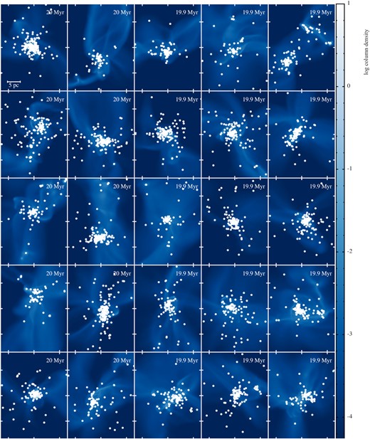
The final state of all simulations that ran to 20 Myr, with sink particles shown in white. The background image is in units of g cm−2. The size of each panel is the same, approximately the size of the initial cloud, and a scale bar of 5 pc is shown in the first panel.
3.1 Number of sinks
Fig. 2 shows the number of sinks formed in each simulation. The mean number of sinks produced in only those that ran to completion is 180 with a standard deviation of 50.
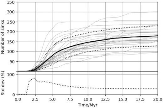
Upper: the number of sinks in each simulation over time are shown in grey. The mean and ±1 standard deviation are shown as the solid and dotted thick lines, respectively. Lower: the standard deviation as a percentage of the mean.
The number of sinks formed in each simulation has a greater variation at early times (58 per cent of the mean at 5 Myr) and then settles to around 30 per cent from 10 Myr onwards. However, as we do not include feedback, these results are less realistic after about 5 Myr as feedback from the young stars would impact later star formation. This is a large variation caused by only changing the random seed, but the exact number of stars is not commonly used as a comparison metric in simulations as it can depend on details such as the sink formation criteria and equation of state.
3.2 Star formation efficiency
Fig. 3 shows how the SFE for each simulation evolves over time, and it is clear that there is a large variation between realizations of the same setup. After only 5 Myr (one free-fall time) the SFE has a standard deviation of 60 per cent of the mean. The maximum variation is at around 7.5 Myr after which it decreases slightly. This standard deviation is very high at earlier times, decreasing rapidly to 10 Myr and then more slowly. We can conclude that the SFE of a single simulation run for less than 10 Myr can depend greatly on the exact details of the initial turbulent field, so any differences caused by changing the initial setup or physical recipes may be hard to detect as a statistically robust result. This may be important for simulations with feedback, which would come into effect after a few Myr when the variance is very high, and may enhance these differences.
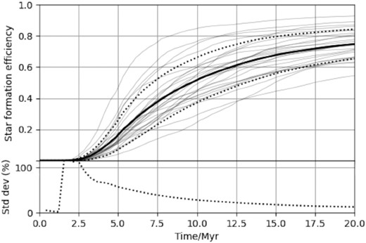
Upper: the variation in the SFE of each simulation (pale grey lines) over time, with the mean of all simulations at each time shown as the solid black line and the standard deviation shown as a black dotted line. Lower: the standard deviation as a percentage of the mean.
We also note that the SFE is sometimes used to define an end point of simulations rather than a set time (e.g. running until 10 per cent of the mass has turned into stars) as a proxy for the quenching of star formation by feedback when feedback processes are not simulated (e.g. Balfour et al. 2015). Due to the spread in SFE this can be at very different times – in this suite of simulations, the time at which 10 per cent SFE is reached can vary by almost 5 Myr. This means that using this cut-off to justify ignoring processes that only have an effect after a certain length of time such as supernovae after the lifetime of a massive star may not be valid. Analytic models often assume that star formation happens on the order of a free-fall time, but we can see that after one free-fall time of this system (5 Myr) the SFE could be anywhere from 10–50 per cent.
3.3 Column density PDF
Theoretical work has predicted that the column densities in a turbulent molecular cloud would have a lognormal probability density function (PDF) with a power-law tail at high column densities where gravity dominates and star formation is ongoing (Vazquez-Semadeni 1994; Ostriker, Stone & Gammie 2001; Tassis et al. 2010; Ballesteros-Paredes et al. 2011). The PDF of molecular cloud column densities has been used in both observational and simulated studies, as well as to compare simulations to observations (Kainulainen et al. 2009; Lombardi, Alves & Lada 2010; Alves, Lombardi & Lada 2014; Donkov, Veltchev & Klessen 2017). There is debate as to whether the lognormal shape is a reliable observational metric as it may be confounded by issues of noise, line-of-sight contamination, or completeness (Ossenkopf-Okada et al. 2016; Alves, Lombardi & Lada 2017), but theoretical work has linked the shape of the lognormal of an individual cloud to important environmental properties, such as the Mach number, type of turbulence, or magnetic pressure (Federrath et al. 2010; Molina et al. 2012).
Fig. 4 shows a selected example of a column density PDF from our simulations, when star formation is ongoing. Our simulations begin with a uniform density sphere with turbulent velocities, so the PDF of each cloud will be identical to start with. As in Ballesteros-Paredes et al. (2011), we expect a lognormal shaped PDF to get wider as the density evolves to match the turbulent velocity field. Then, as dense regions undergo gravitational collapse and star formation begins, the PDF should develop a power-law tail. We have observed this widening trend in our data but not fitted a lognormal to quantify this. Ward, Wadsley & Sills (2014) find that the power-law tail appears at approximately 0.5tff, and the peak shifts to lower density as the lognormal shape widens (although they note this is not an effect of gravitational collapse as this happens in pure hydrodynamic simulations as well). They find that the slope of the power-law tail increases over time converging on a value around −2 in simulations with a range of initial conditions. We fitted a power-law tail to our PDFs using the Plfit Python package by A. Ginsburg based on the statistical work of Clauset, Shalizi & Newman (2009). All fits are tested using a bootstrap method to ensure that the power-law fit is valid.2
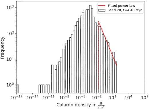
An example of the column density PDF of a selected snapshot, showing the fitted power law as a red solid line and the minimum value the power law extends to as a red dashed line.
Fig. 5 shows the slope fitted to the high mass end of the column density PDFs of our simulations over time. Note that this graph only extends to 10 Myr rather than the full 20 Myr, as the fitting procedure is computationally intensive and there was little change in structure after 10 Myr. We can clearly see the slope of the power-law tail decreasing with time, although it converges to a smaller value than Ward et al. (2014) report, reaching a mean of −1.62 at 10 Myr with a standard deviation of 9 per cent of the mean. This is known to depend on the sonic Mach numbers and the type of turbulence forcing (see fig. 4 in Federrath & Klessen 2013), so we do not expect to find exactly the same value as Ward et al. (2014). We find that the slopes are fairly constant from 5 Myr onwards, suggesting that the cloud structure does not evolve significantly after that point. Looking at Figs 2 and 3, we can see that most of the stars are formed in the first 5 Myr, so the change in the slope of the column density PDF is clearly related to ongoing gravitational collapse and star formation.
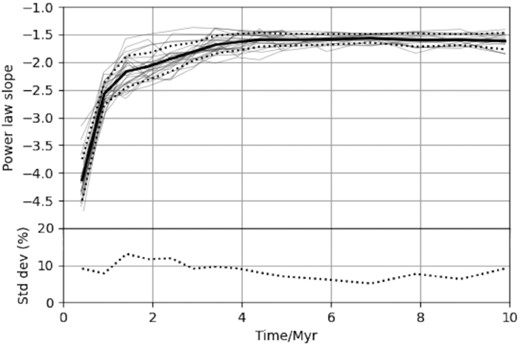
Upper: the fitted power-law slope of each simulation (thin grey lines) over time, with the mean of all simulations shown as a solid black line and the standard deviation as a dotted black line. Lower: the standard deviation as a percentage of the mean.
4 CONCLUSIONS
We have performed a suite of simulations of a turbulent molecular cloud collapsing under gravity to form a star cluster. The initial conditions of each simulation are identical except for the random number used to generate the turbulent field. The turbulent field has the same bulk properties (power spectrum, solenoidal versus compressive modes, total energy) while changing the exact velocity of each particle in the initial conditions. As star formation is a mathematically chaotic process, these small differences are amplified and the simulations diverge. The results after only 1 free-fall time are significantly different, and by the end of the simulations are very different. We note that the number of sinks formed is highly variable, the SFE is quite variable, and the power-law slope of the column density PDF is much more reliable.
Simulations are often used to test how a change in initial conditions or numerical recipes for different physics impacts star formation. This can be measured by many metrics, including the number of stars (or sinks) formed, the amount of gas turned into stars (SFE) and the distribution of gas column densities, quantified by fitting a power law to the column density PDF. We find that all of these can vary without changing any of the commonly investigated parameters of initial conditions, such as the size or shape of cloud or the physical recipes included, and therefore any single realization will not represent the range of possible values of that setup. Our simulations are quite simple in order to keep runtimes low, so we do not expect the exact values to be representative. In Table 1 we give the standard deviation as a percentage of the mean and propose that this be applied as an error bar to any measurement from a single simulation. This will enable results from single realization simulations to be robustly compared and any changes found when new physics is included must be larger than this to be significant.
The average and range of each value we measured over time, presented as ‘mean ± standard deviation (standard deviation as percentage of mean)’. Note that only the simulations that ran to 20 Myr are included, and for the power-law slope we only analyse up to 10 Myr, for reasons of computational efficiency.
| Time (Myr) | Number of sinks | Star formation efficiency | Power-law slope of column density PDF |
|---|---|---|---|
| 5 | 78 ± 45 (58 per cent) | 0.15 ± 0.09 (60 per cent) | −1.59 ± 0.11 (7 per cent) |
| 10 | 145 ± 47 (32 per cent) | 0.51 ± 0.15 (29 per cent) | −1.62 ± 0.15 (9 per cent) |
| 15 | 169 ± 49 (29 per cent) | 0.67 ± 0.12 (18 per cent) | – |
| 20 | 180 ± 50 (28 per cent) | 0.75 ± 0.09 (12 per cent) | – |
There are many physical processes that impact star formation, and large computationally intensive simulations that include as much physics as possible or have very high resolution are vital to investigate these processes. However, any single simulation cannot be simply assumed to represent a general picture of star formation under similar conditions, and must include these uncertainties on results to account for the chaotic variation inherent in these highly non-linear systems. We would encourage all simulators to perform as many repeated realizations as possible, as these effects will be influenced by the choice of code and inclusion of other physical processes.
ACKNOWLEDGEMENTS
We are grateful for the help of Christoph Federrath, Sam Geen and Matthew Bate in useful discussion and sharing data. The simulations were performed on the University of Hertfordshire’s UHHPC cluster. SJ acknowledges support from the UK Science and Technology Facilities Council (STFC) grant ST/R000905/1. SDC is supported by the Ministry of Science and Technology (MoST) in Taiwan through grant MoST 108-2112-M-001-004-MY2.
DATA AVAILABILITY
The data underlying this article will be shared on reasonable request to the corresponding author.
Footnotes
We note that some simulation codes have an option to sub-cycle close binaries, to evolve them on a smaller time-step without major delays to the rest of the evolution. This would enable such dense stellar systems to be studied more efficiently.
We note that the standard goodness-of-fit test used in astronomy – performing a K–S test and comparing the p-value to tabulated values – is not applicable in this case as the distribution we want to test is fitted to the data, so the bootstrap test must be used instead. However, since the p-value is so commonly misused as to be almost universal, we note that most of the fits would fail this test at early times (<1 Myr) and pass from then on.
