The nozzle shock in tidal disruption events Free

ABSTRACT

1 INTRODUCTION

Stars near the centre of galaxies occasionally get launched on a plunging near-parabolic trajectory that leads to their disruption by the strong tidal forces of the central supermassive black hole. This phenomenon called tidal disruption event (TDE) results in the formation of a debris stream that progressively fuels the compact object, leading to strong electromagnetic emission outshining the entire host galaxy (Rees 1988). This signal represents a powerful probe of the majority of supermassive black holes in the our local Universe that are otherwise starved of accreting material, and therefore undetectable.

Many TDE candidates have already been discovered as powerful flares of radiation lasting from months to years and originating from the innermost region of otherwise quiescent galaxies. This emission can cover a wide range of the electromagnetic spectrum, which usually includes components in the optical/ultraviolet (UV) or the soft X-ray bands (Komossa et al. 2008; Gezari et al. 2012; Chornock et al. 2014; Leloudas et al. 2016, 2019; Gezari, Cenko & Arcavi 2017; Saxton et al. 2017; Holoien et al. 2019; van Velzen et al. 2019; Hung et al. 2020; Short et al. 2020) that likely have different physical origins. Several of these observations additionally present strong evidence of matter present on large scales with outflowing motion, which is expected given the violent interactions that the stellar matter can undergo as it reaches the vicinity of the black hole to eventually get accreted.

The stellar disruption itself is overall well understood that makes quantitative predictions possible for the hydrodynamics of this early phase. For deep encounters, this process may be accompanied by strong compression potentially triggering nuclear reactions, as first proposed by Carter & Luminet (1982). The stellar debris then evolves into an elongated stream, whose transverse profile can be confined by the gas self-gravity (Kochanek 1994; Coughlin & Nixon 2015; Coughlin et al. 2016b; Steinberg et al. 2019). About half of this stream is bound to the black hole, thus returning to its vicinity according to a predictable fallback rate (Evans & Kochanek 1989; Lodato, King & Pringle 2009; Guillochon & Ramirez-Ruiz 2013) that chiefly depends on the stellar structure. However, the gas is not expected to emit observable radiation¹ until it passes at pericentre for the second time.

Starting from the return of this matter to the black hole, our understanding of the hydrodynamics becomes much less secure. The main difficulty is a computational one that prevents from accurately following the pericentre passage of the stream within a global three-dimensional simulation. An early simulation by Lee & Kim (1996) displays a large expansion of the gas at this location that they suspect could be caused by a lack of resolution. Later on, Ayal, Livio & Piran (2000) similarly find that the gas gets strongly heated during pericentre passage, which has the more extreme consequence of unbinding most of the mass. It now appears likely that the gas evolution found in these works is significantly affected by numerical artefacts caused by a too low resolution. This issue at least partly stems from the fact that the stream of debris displays a very large aspect ratio with a longitudinal extent larger than its transverse width by several orders of magnitude, which makes it difficult to discretize with enough resolution elements in both directions. Although numerical errors seem to become less catastrophic when resolution is improved, there is so far no convincing evidence that the problem completely disappears, even when approaching the limit of currently available computational resources.

In order to alleviate this computational burden, most numerical investigations have so far relied on simplifications of the problem compared to the physically motivated situation involving a parabolic stellar trajectory and supermassive black hole (for a recent review, see Bonnerot & Stone 2021). This is usually achieved by decreasing either the stellar eccentricity (Hayasaki, Stone & Loeb 2013; Bonnerot et al. 2016; Sadowski et al. 2016) or the black hole mass (Rosswog, Ramirez-Ruiz & Hix 2009; Guillochon, Manukian & Ramirez-Ruiz 2014; Shiokawa et al. 2015), which both tend to reduce the longitudinal size of the stream, making it numerically easier to resolve. The advantage of these simulations is that they can follow the global evolution of the gas in three dimensions. In particular, they capture the self-crossing shock induced by relativistic precession that results from an intersection between the part of the stream going away from the black hole after pericentre passage and that still moving inward. These works find that this collision can initiate the formation of an accretion flow, which is likely associated with most of the radiation observed from TDEs. However, it is not generally possible to extrapolate these results obtained for simplified initial conditions to the more physically realistic situation. More recently, Andalman et al. (2022) performed a simulation that does not rely on these simplifications, but still considers a less likely deeply penetrating disruption. Because of the high computational needs involved, the gas could however only be followed for a short duration even making use of their efficient GPU-accelerated code.

In another class of works, the authors have chosen to treat the passage of the stream near the black hole in an analytical way, which is most commonly achieved by assuming that the centre of the stream evolves ballistically with either a full or approximate calculation of general relativistic geodesics (Dai, Escala & Coppi 2013; Dai, McKinney & Miller 2015; Guillochon & Ramirez-Ruiz 2015; Bonnerot, Rossi & Lodato 2017a; Lu & Bonnerot 2020). Such calculations were mainly used to determine the properties of the two stream components involved in the self-crossing shock. This first interaction was then studied by means of local simulations (Lee, Kang & Ryu 1996; Kim, Park & Lee 1999; Jiang, Guillochon & Loeb 2016; Lu & Bonnerot 2020) to determine the properties of the resulting outflow. Making use of this information, Bonnerot & Lu (2020) were able to perform the first simulation of the subsequent accretion disc formation for astrophysically realistic parameters, by treating the outflow through an injection of matter. However, a significant uncertainty in the above analytical treatments concerns the level of stream expansion occurring during pericentre passage. This effect could lead to different properties for the colliding streams, which may reduce the efficiency of the self-crossing shock and cause the outflow to become less spherical than for identical streams (see fig. 3 of Bonnerot & Stone 2021 for an illustration of this difference). This mechanism is also fundamental if the black hole has a non-zero spin, which can cause the streams to be offset at the intersection point due to relativistic nodal precession. While the collision may be entirely missed if the streams are both very thin, some of the gas could nevertheless collide if the vertical offset is compensated by an increase in stream thickness (Dai et al. 2013; Guillochon & Ramirez-Ruiz 2015; Hayasaki, Stone & Loeb 2016; Liptai et al. 2019).

The main interaction taking place when the stream passes near the black hole is usually referred to as a ‘nozzle shock’. It results from a strong vertical compression induced by an intersection of the orbital planes of the returning gas near pericentre. This phenomenon is similar to that involved in the process of deep stellar disruption, during which the entire star gets squeezed (Carter & Luminet 1982; Luminet & Marck 1985; Brassart & Luminet 2008; Stone, Sari & Loeb 2013). However, the nozzle shock has not received as much attention so far. One of the earliest investigations of this process has been done in the pioneering work by Kochanek (1994) that studies the stream evolution at pericentre in a semi-analytical way. In analogy with the case of deep disruptions, analytical estimates by Guillochon et al. (2014) suggest that the specific kinetic energy dissipated by the nozzle shock is of order the squared stellar sound speed. This conclusion has been used to formulate an analytical prescription for the resulting stream expansion in the semi-analytical study by Guillochon & Ramirez-Ruiz (2015) that focuses on the impact of black hole spin. The nozzle shock has also been captured by three-dimensional simulations of stellar disruption by low-mass black holes (Ramirez-Ruiz & Rosswog 2009; Shiokawa et al. 2015) or involving deep penetrations (Sadowski et al. 2016) but without a detailed analysis of the underlying mechanism. More recently, it has also been studied in the context of eccentric accretion discs through a semi-analytical treatment of this type of flows (Zanazzi & Ogilvie 2020; Lynch & Ogilvie 2021a,b).

In this paper, we perform the first systematic study dedicated to the nozzle shock in TDEs. Our approach consists in first simulating the stellar disruption in three dimensions to obtain the property of a given section of the fallback stream. To circumvent numerical issues encountered in past works, the subsequent evolution of this stream element is studied with a two-dimensional simulation. This is achieved thanks to a method we developed that follows the dynamics of this gas along the two transverse directions in the frame comoving with its centre of mass and corotating with the local direction of stream elongation. With this technique, we are able to study the hydrodynamics of this stream element throughout its evolution around the black hole at sufficient resolution, including the passage at pericentre where the nozzle shock occurs.

This paper is arranged as follows. In Section 2, we describe our initial conditions and the numerical method used to follow the transverse evolution of a stream element in two dimensions. The results of this simulation are presented in Section 3, from the gas infall towards pericentre where the nozzle shock takes place to the subsequent recession of this matter back to larger distances. In Section 4, we carry out a convergence study, demonstrate the validity of our two-dimensional treatment, determine the consequences of our results on the later stages of evolution, and evaluate the impact of several additional physical processes on the nozzle shock. We include a summary of our main findings in Section 5.

2 MESHLESS SIMULATIONS

Our numerical strategy consists first in performing a three-dimensional simulation of stellar disruption, from which we obtain the properties of a given section of stream. The subsequent transverse evolution of this stream element is then followed in two dimensions as it continues to approach the black hole.

2.1 Initial conditions

The stellar disruption is followed with the hydrodynamics code gizmo (Hopkins 2015), making use of the meshless finite mass technique that consists in dividing the gas into particles of fixed mass. The star has a solar mass and radius with a density profile assumed to be polytropic with an exponent γ_⋆ = 5/3. It is constructed by first placing the particles in a closed-pack lattice and then radially stretching their position to obtain the desired profile. This distribution is then evolved for a few dynamical times including a damping term until the amplitude of its oscillations become negligible. We use N_D = 10⁷ particles with mass |$M_{\rm D} = 10^{-7} \, \mathrm{M}_{\rm{\odot }}$| that is among the largest resolution used for this type of study. The star is initially placed at a distance R₀ = 3R_t from the black hole on a parabolic orbit with pericentre equal to the tidal radius of equation (1). Self-gravity is included to simulate the encounter and the gas is assumed to follow an adiabatic equation of state with γ = 5/3 as expected for this phase of evolution. A Newtonian potential is used to describe the black hole’s gravity, which amounts to neglecting the impact of general relativity. This approximation is justified by the fact that the pericentre of the orbit is much larger than the gravitational radius, with a ratio of R_p/R_g ≈ 47 ≫ 1. Gas particles that get within an accretion radius R_acc = 3R_t from the black hole are removed from the simulation.

In this initial phase, the gas evolution is similar to that found in previous studies (Lodato et al. 2009; Guillochon & Ramirez-Ruiz 2013; Guillochon et al. 2014; Coughlin & Nixon 2015), and we therefore only provide a brief description. Following the encounter, the stellar debris gets imparted a spread in orbital energy a few times larger than that |$\Delta \epsilon = G M_{\rm h}R_{\star }/ R_{\rm t}^2$| analytically expected from the frozen-in approximation (Stone et al. 2013). Half of this gas gets bound to the black hole with its extremity coming back the earliest to pericentre, after a time slightly shorter than |$t_{\rm min}= 2 \pi G M_{\rm h}(2 \Delta \epsilon)^{-3/2} \approx 41 \, \rm d$| according to Kepler’s third law. The tip of the returning stream can be seen from the gas density shown at a time t/t_min = 0.59 since disruption in the left-hand panel (a) of Fig. 1. At large radii, the stream displays a thin profile due to its confinement by self-gravity following the disruption (Kochanek 1994; Coughlin et al. 2016b). Because it originates from the stellar outermost layers, the gas closer to the black hole is more tenuous, which reduces the impact of self-gravity. As a result, this more bound matter presents, in addition to the central part, a wing several orders of magnitude less dense that extends towards the left. This asymmetry and wider range of densities makes the transverse gas properties of this part of the stream more difficult to describe and to accurately follow numerically. For this reason, we choose to study instead the near-cylindrical and more compact gas that arrives immediately after. The specific element we select to follow its later evolution around the black hole is indicated with the red point in Fig. 1.

Figure 1.

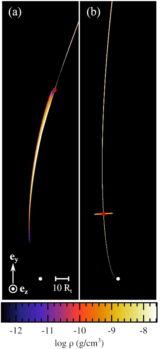
Snapshots taken from the preliminary three-dimensional simulation of stellar disruption, showing the gas density inside the tip of the stream of debris as it falls back towards the black hole at times t/t_min = 0.59 (left-hand panel) and 2.2 (right-hand panel). The value of the density increases from black to white, as shown on the colour bar. The white segment on the first snapshot indicates the scale used and the orientation is given by the white arrows. The red dot indicates the location of the stream element selected to follow its transverse evolution at later times as it continues to move towards the black hole. Its properties are recorded at the time of the second snapshot when it reaches the surface depicted with the orange segment that is orthogonal to the longitudinal stream direction.

Open in new tabDownload slide

This element has an orbital energy ϵ = −0.575Δϵ that corresponds to a fallback rate of |$\dot{M}= 0.685 \, \rm \mathrm{M}_{\rm{\odot }} \, {yr}^{-1}$|⁠, only a factor of ∼2 lower than the peak value. Note that this choice is mostly made for computational convenience but we discuss its possible influence on our results in Section 4.3. The two-dimensional transverse properties of the element are recorded at t/t_min = 0.22 when it reaches a distance R_in = 51.2R_t from the black hole. This is done by defining a surface orthogonal to the stream longitudinal direction at this location, which is displayed with the orange segment on the right-hand panel (b) of Fig. 1. The properties of a few hundred particles are recorded as they cross this surface, which are used to determine by interpolation the transverse profiles of the hydrodynamical variables. The location of a given particle on this surface is parametrized by the two coordinates ξ and z shown in the sketch of Fig. 2 that correspond to offsets with respect to the centre of mass along the stellar orbital plane and the vertical direction, respectively.

Figure 2.

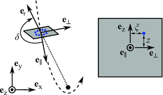
Sketch illustrating the two-dimensional treatment used to follow the transverse evolution of a stream element around the black hole. The particles (blue points) used to describe the gas are confined at all times to the grey surface, which follows the trajectory (dashed line) of its centre of mass while remaining orthogonal to the longitudinal direction of the stream defined by the unit vector |$\boldsymbol {e}_{\parallel }$|⁠. This direction makes an angle δ < 0 with the outward radial direction, which evolves in time as the stream element moves. The transverse position of a given particle is specified by the coordinates ξ and z that correspond to offsets with respect to the centre of mass along the in-plane and vertical directions specified by the unit vectors |$\boldsymbol {e}_{\perp }$| and |$\boldsymbol {e}_{\rm z}$|⁠, respectively.

Open in new tabDownload slide

The initial density profile can be approximated by a binormal distribution ρ_in(ξ, z) = Λ(2|$\pi$|σ_⊥σ_z)⁻¹ exp (−((ξ/σ_⊥)² + (z/σ_z)²)/2), with fitted values of the standard deviations of σ_⊥ = 4.1R_⋆ and σ_z = 2.0R_⋆. Note that this element is narrower along the vertical direction, which is caused by earlier oscillations around hydrostatic equilibrium seeded by the passage of the star at pericentre (Coughlin et al. 2016a). To ensure that the density distribution is consistent with the fallback rate, the normalization is fixed by |$\Lambda = \int _{-\infty }^{\infty } \int _{-\infty }^{\infty } \rho _{\rm in}(\xi ,z) \mathop {}\!\mathrm{d}\xi \mathop {}\!\mathrm{d}z = \dot{M} / v_{\rm c, in}$|⁠. The centre of mass speed has a value of v_{c, in} = 16.6v_⋆, where |$v_{\star } = \sqrt{G M_{\star }/ R_{\star }} = 440 \, \rm km \, s^{-1}$| denotes the approximate stellar sound speed, such that the central density is given by |$\rho _{\rm in}(0,0) = \dot{M}/ (2 \pi v_{\rm c, in} \sigma _{\perp } \sigma _{\rm z}) = 2.4 \times 10^{-7} \, \rm g \, cm^{-3}$|⁠. Because of the proximity to the black hole, the centre of mass has its velocity completely aligned with the stream longitudinal direction,² which itself is almost along the inward radial direction. Specifically, these two directions are initially inclined by an angle δ_in ≈ −0.95|$\pi$| < 0 (see Fig. 2). The initial velocity profiles in the comoving frame can be approximated by homologous transverse compression along both directions given by v_{z, in}/v_{c, in} = A_{z, in}z/R_in and v_{⊥, in}/v_{c, in} = A_{⊥, in}ξ/R_in, where A_{z, in} = −0.47 and A_{⊥, in} = −0.39 are obtained by fitting. Similarly, the longitudinal velocity changes across the stream as v_{∥, in}/v_{c, in} = A_{∥, in}ξ/R_in with A_{∥, in} = 0.12 > 0 since the material with ξ > 0 is closer to the black hole. As representative examples, Fig. 3 shows the initial density (upper panel) and vertical velocity (lower panel) profiles along the orbital plane and orthogonal to it, respectively. The orange dots correspond to the particles picked from the three-dimensional simulation that are used for the interpolation, while the red lines are the fitted profiles. For simplicity, we adopt a uniform specific thermal energy distribution given by its average value of |$u = 4.8 \times 10^{-6} v^2_{\star }$| for the selected particles. Note that the corresponding gas temperature |$T = 2 m_{\rm p} u /(3 k_{\rm B}) \approx 70 \, \rm K$| is very small, which in reality may be prevented by hydrogen recombination that injects energy into the gas at earlier times (Coughlin et al. 2016b). This choice is nevertheless appropriate because pressure forces are found to be irrelevant until the gas reaches close to pericentre where strong heating occurs that makes the matter forget about its initially much lower internal energies.

Figure 3.

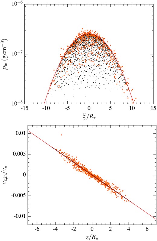
Initial density (upper panel) and vertical velocity (lower panel) profiles inside the stream element along the in-plane and vertical directions, respectively. The orange dots correspond to individual particles selected from the three-dimensional simulation of stellar disruption that are used to obtain the fitted profiles shown with the red lines. The smaller black dots correspond to the particles used as initial conditions of the two-dimensional simulation, whose properties are determined by the fitted profiles. We only display |$1{{\ \rm per\ cent}}$| of the N_p ≈ 2 × 10⁵ particles used in the simulation so that individual points can be distinguished.

Open in new tabDownload slide

The initial conditions of the two-dimensional simulation are then created by generating a higher resolution version of this stream element along the orthogonal surface. The initial mass of gas is |$m_{\rm in} = \Lambda l \approx 2 \times 10^{-6} \, \mathrm{M}_{\rm{\odot }}$|⁠, which is specified by a longitudinal length arbitrarily fixed to l = R_⋆. Even though the gas only has a surface density Σ defined on the orthogonal surface, it can be converted into a three-dimensional density given by ρ = Σ/l, which is used instead throughout the paper. Importantly, this density is independent of our choice of length l since this parameter affects the mass and enclosing volume in the same proportional way. The particle mass M_p specifies the number of particles used in the simulation given by N_p = [m_in/M_p], where the brackets denote the nearest integer function. We choose a value of |$M_{\rm p} = 10^{-11} \, \mathrm{M}_{\rm{\odot }}$| corresponding to N_p ≈ 2 × 10⁵ particles. In Section 4.1, we determine the influence of resolution on our results to demonstrate that the above particle number is enough to attain numerical convergence.

The particles are first positioned randomly on the orthogonal surface according to the probability distribution associated with the binormal function fitted for the density. To reduce density interpolation errors resulting from random noise, we find it necessary to relax the particle distribution. This is realized by evolving the gas for a short duration inside a periodic box whose vacuum is filled with ghost particles to prevent artificial expansion. To impose the particles to move towards the desired density profile, they are also subject to a pressure force that vanishes when this configuration is attained. After the particles have reached their final position, we assign their velocities according to the fitted profiles and its uniform specific internal energy. The result of this procedure is displayed with the black points in Fig. 3, which by comparison with the red lines demonstrates that the gas properties are correctly imposed. The stream element thus obtained is then used to initialize a two-dimensional simulation that studies its transverse gas evolution at later times, according to the numerical method we now explain.

2.2 Two-dimensional treatment of hydrodynamics

We aim at studying the two-dimensional transverse evolution of the selected stream element during its passage near the black hole in the frame comoving with its ballistic centre of mass and corotating with the local longitudinal direction of elongation. We rely on the orientation indicated in Fig. 2 that is specified by three orthogonal unit vectors |$\boldsymbol {e}_{\parallel }$|⁠, |$\boldsymbol {e}_{\perp }$|⁠, and |$\boldsymbol {e}_{\rm z}$|⁠, aligned with the longitudinal direction and along the two transverse ones, respectively. The stream element has its longitudinal direction aligned with the velocity |$\boldsymbol {v}_{\rm c}$| of its centre of mass such that |$\boldsymbol {e}_{\parallel } = \boldsymbol {v}_{\rm c} / v_{\rm c}$|⁠, where |$v_{\rm c} = |\boldsymbol {v}_{\rm c}|$|⁠. The orientation of the above unit vectors is then specified at all times by this velocity, which we evaluate along with the position |$\boldsymbol {R} = R \boldsymbol {e}_{\rm r}$| of the centre of mass, assuming that it follows a Keplerian orbit under the gravitational acceleration |$\boldsymbol {a}_{\rm c} = -G M_{\rm h}\boldsymbol {R} / R^3$|⁠. Here, |$R = |\boldsymbol {R}|$| while |$\boldsymbol {e}_{\rm r}$| is a unit vector pointing outward in the radial direction.

We assume that the gas thermodynamical evolution is adiabatic with γ = 5/3. This is justified by the inability of the gas to significantly cool through radiation due the large optical depths involved, as demonstrated in Section 4.8. Additionally, the gas pressure dominates that provided by radiation with a ratio of P_rad/P_gas = (aT⁴/3)/(ρk_BT/m_p) ≲ 0.01. Anticipating the results, this numerical value uses the maximal temperature and density of |$T \approx 10^6 \, \rm K$| and |$\rho \approx 10^{-3} \, \rm g \, cm^{-3}$| reached by the gas throughout its evolution. Shocks are treated in gizmo by solving the Riemann problem at faces reconstructed at the boundaries between particles. This is done by using the numerical scheme proposed by Panuelos, Wadsley & Kevlahan (2020), which we choose for its ability to maintain good particle order, as required for our problem. The gas contained in the element initially satisfies |$\rho _{\rm in} \lt M_{\rm h}/(2 \pi R^3_{\rm in}) = 1.2 \times 10^{-6} \, \rm g \, cm^{-3}$| (see upper panel of Fig. 3), implying that self-gravity is overwhelmed by the tidal force (Coughlin et al. 2016b). Because this is also the case closer to the black hole, the gas self-gravity is not taken into account in the two-dimensional simulation.

2.3 Ballistic motion of the stream element

Before presenting the hydrodynamical results, we start by better characterizing the ballistic motion of the gas. The centre of mass trajectory of the stream element is shown with the black solid line in Fig. 4, which starts at the orthogonal surface represented by the orange segment, where the two-dimensional simulation is initialized. The pericentre of this trajectory is denoted by the black diamond in the lowermost inset, whose location is essentially identical⁵ to that R_p = R_t of the star due to the small angular momentum spread imparted by the stellar disruption (Cheng & Bogdanović 2014). The orbital energy of the selected element specifies its semimajor axis a ≈ 87R_t, which corresponds to a high eccentricity e ≈ 0.99. Before reaching the initial orthogonal surface, the stream element was moving on the trajectory indicated with the black dotted line obtained by backwards integration of a Keplerian orbit. We find that the tidal force overcomes the stream self-gravity during this earlier phase at a distance R_eq  ≈ 1.8a from the black hole. This location is indicated by the grey point while the arrow of the same colour represents the direction of the corresponding velocity vector. The gas is still close to hydrostatic equilibrium at this moment but starts getting tidally compressed as it continues to move inward.

Figure 4.

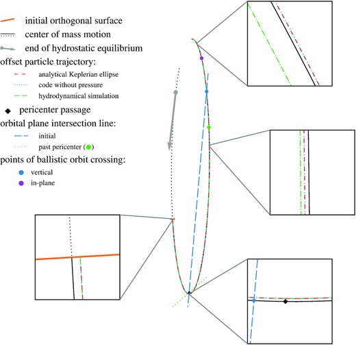
Trajectories followed by different parts of the selected stream element during its passage near the black hole (black dot). Differences between them can be distinguished from the four rectangles that are insets zooming-in on specific regions. The black solid line represents the centre of mass trajectory, starting from the orthogonal surface (orange segment) where the two-dimensional simulation is initialized. Its pericentre is indicated by the black diamond in the lowermost inset, which is located close to that of the star. The dotted black curve represents the same trajectory at earlier times, as obtained by backward integration. The grey point shows the location where the tidal force overcomes the gas self-gravity, while the arrow of the same colour represents the orientation of the corresponding velocity vector. We consider a single particle inside the stream element with initial relative positions ξ ≈ 5R_⋆ and z ≈ 2R_⋆, and velocities given by the fitted homologous profiles. Its trajectory is shown with the coloured curves that are computed in different ways: analytically from a Keplerian ellipse (red dashed line) and by integrating equations (4) and (5) with pressure forces switched off (blue dotted line). These two orbits perfectly overlap as seen from the insets, which proves the correct implementation in gizmo. The particle considered evolves on an orbital plane inclined with respect to that of the centre of mass. These two planes intersect along the blue long-dashed line, which is parallel to the grey velocity vector, as expected geometrically. The stream collapses vertically when it crosses this line at the location of the blue points. This happens for example slightly before pericentre as seen from the lowermost inset, which is where the nozzle shock is expected to take place. The green dash–dotted line shows the trajectory of the exact same initial particle but including pressure forces from the rest of the matter within the stream element. It deviates from the two other ballistic orbits (red dashed and blue dotted lines) past pericentre, as seen from the two uppermost insets. The intersection line of its orbital plane with that of the centre of mass is shown with the green dotted line, which is evaluated when the stream element has reached the green point.

Open in new tabDownload slide

The coloured curves correspond to the trajectory of a single particle belonging to the stream element whose relative positions are initially of ξ ≈ 5R_⋆ and z ≈ 2R_⋆ with velocities given by the fitted profiles. The red dashed line is evaluated analytically as a Keplerian ellipse from these initial conditions. The blue dotted line is obtained in a very different way by using the method described in Section 2.2, switching off pressure forces in equations (4) and (5). These two trajectories completely overlap, as can be seen from all the insets. Similarly, the vertical motion is found to be identical using the two methods of calculation. This proves the correct implementation of the numerical solution designed to follow the transverse gas evolution with gizmo and the validity of the tidal approximation used in equation (3). The green dash–dotted line displays the trajectory of the exact same initial particle but taking into account pressure forces. It can already be seen to deviate from the ballistic trajectories, as we describe in detail in Section 3.

The gas inside the stream element with an initial vertical offset evolves on orbital planes inclined with respect to that of the centre of mass. These planes intersect along the same line for all the gas owing to the homologous nature of the compression (Stone et al. 2013). It is shown with the blue long-dashed line in Fig. 4 that is obtained from the test particle considered above. As we further explain in Appendix  C, its orientation must be parallel to the velocity vector of the stream when the tidal force starts dominating self-gravity, which we indeed find to be the case by comparing with the grey arrow. This geometrical construction was already noticed in the early work of Luminet & Marck (1985) in the context of deep stellar disruptions. The stream gets vertically compressed⁶ when it crosses this line at the location of the blue points. This occurs for example slightly before pericentre passage, as seen from the lowermost inset of Fig. 4. The stream is expected to reach its maximal level of compression near this location that is at the origin of the nozzle shock. Another consequence is that the orbital planes intersect close to apocentre, which would lead to another vertical collapse of the stream element, but only if its evolution is entirely ballistic during and after pericentre passage.

The situation is different for the in-plane motion since the fluid elements never intersect with the trajectory of the centre of mass during the infalling motion. This is because the gas with ξ > 0 has a lower pericentre distance than the centre of mass (see lowermost inset in Fig. 4), which is permitted by a change of sign of the in-plane acceleration.⁷ However, ballistic motion implies that an intersection does take place along the stellar orbital plane after pericentre passage. Its exact location is displayed with the purple point in Fig. 4 located slightly before the apocentre of the trajectory. Looking at the two insets directly before and after this point, it is clear that the ballistic trajectories (red dashed and blue dotted lines) have changed side compared to that of the centre of mass (black solid line). As explained further in Appendix  C, this intersection mainly results from the initial conditions that impose a slightly larger apocentre distance for fluid elements with ξ > 0.

3 RESULTS

We now present the results of the simulation following the transverse gas evolution in the stream element.⁸ This is done in a chronological manner, particularly focusing on the nozzle shock taking place near pericentre.

3.1 Approach to the black hole

We start by briefly describing the evolution of the stream element found in the three-dimensional simulation of disruption. Fig. 5 shows with dotted lines its transverse widths (upper panel) and density (lower panel) as a function of distance from the black hole during this early phase, from shortly after the stellar disruption (diamonds) to the beginning of the fallback. Both the vertical (black dotted line) and in-plane (red dotted line) widths increase on average according to the scaling H ∝ R^1/2 (grey segment), which is expected from gas in hydrostatic equilibrium with self-gravity compensating gas pressure forces for an adiabatic evolution with γ = 5/3 (Coughlin et al. 2016b). In addition, the stream displays oscillations that are almost exactly out-of-phase between the two transverse directions, which implies that the stream gets deformed according to an approximately quadrupolar mode. We attribute these oscillations to in-plane pancake shocks taking place during the stellar disruption, as proposed by Coughlin et al. (2016a). During this outgoing phase, the density is expected to evolve as ρ ∝ (H²ℓ)⁻¹ ∝ R⁻³, which is indeed what we find from the simulation (grey segment). This comes from using the width scaling and the fact that the longitudinal extent of a portion of stream with fixed mass increases due to stretching as ℓ ∝ R² (Coughlin et al. 2016b). After reaching its apocentre, the stream element proceeds to move inwards again, which corresponds to a turnaround in Fig. 5. The density then gets lower than the critical value ρ_sg = M_h/(2|$\pi$|R³) (blue dashed line), causing the tidal force from the black hole to become larger than the stream self-gravity and pressure forces. The gas therefore starts moving ballistically under external gravity from this radius of R = R_eq  ≈ 1.8a indicated with the blue arrow in the lower panel, corresponding to the grey point of Fig. 4.

Figure 5.

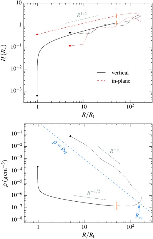
Widths (upper panel) and density (lower panel) of the selected stream element as a function of distance from the black hole as it evolves from shortly after the stellar disruption (diamonds) to its return to pericentre (circles). The density is averaged over the element, while the widths are defined as the distance from the centre of the stream that encloses half of its mass along the vertical (black line) and in-plane (red line) direction. The early phase of outgoing motion and early fallback past apocentre (dotted lines) is obtained from the preliminary simulation of disruption performed in three dimensions. The gas used to compute the above properties has its orbital energies inside a narrow interval centred around that ϵ = −0.575Δϵ of the stream element considered. To compute the widths, we determine the line crossing the centre of this element from the positions of a small portion of gas located at its extremities. The subsequent phase of infall (solid black and dashed red lines) is evaluated from the two-dimensional simulation that starts at the location of the orange vertical segments where the transverse properties of the stream element are recorded. The dashed blue line in the lower panel delimits the region inside which the tidal force from the black hole dominates the stream self-gravity, which is given by ρ_sg = M_h/(2|$\pi$|R³) (Coughlin et al. 2016b). It is reached by the stream element at a radius R = R_eq  ≈ 1.8a indicated by the blue arrow. The grey long-dashed segments indicate the scalings that the widths and density are analytically expected to follow in each phase.

Open in new tabDownload slide

The remaining of the gas evolution is followed with a two-dimensional simulation that starts at the location of the orange vertical segments in Fig. 5. During this phase, the vertical (black solid line) and in-plane (red dashed line) widths still follow H ∝ R^1/2, but the physical reason for this scaling is different from before. It is due to the fact that the transverse motion is entirely ballistic such that the compression takes place with homology factors that tend to A_z = A_⊥ = −0.5, as explained in Section 2.3. This compression causes the density (black solid line) to increase towards lower radii as ρ ∝ R^−1/2 because |$\rho = \dot{M}/(\pi H^2 v_{\rm c})$|⁠, where the centre of mass velocity scales as v_c ∝ R^−1/2 for a near-parabolic trajectory. This compression is directly visible in the first two snapshots of Fig. 6, which show the gas density along the orthogonal surface at the start of the simulation when (t − t_p)/t_⋆ = −197 and later during the infalling phase at (t − t_p)/t_⋆ = −15.6. Here, |$t_{\star }= R_{\star }/v_{\star } \approx 0.44 \, \rm h$| denote the stellar dynamical time-scale, while t = t_p corresponds to pericentre passage. The above scalings imply that the tidal force evolves as F_t ≈ GM_hH/R³ ∝ R^−5/2 and pressure forces as F_p ≈ P/(Hρ) ∝ R^−5/6, such that their ratio scales as F_t/F_p ∝ R^−5/3. This confirms the expectation that the gas transverse motion keeps being specified by external gravity as the stream element continues to approach the black hole. At R ≲ 2R_t, it can be seen from Fig. 5 that the scalings we just derived break down due to a much faster vertical compression at the origin of the nozzle shock.

Figure 6.

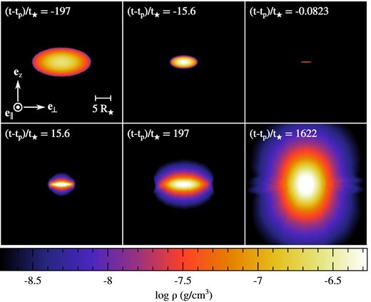
Snapshots showing the gas density inside the stream element along the surface orthogonal to its longitudinal direction at different times (t − t_p)/t_⋆ = −197, −15.6, −0.0823, 15.6, 197, and 1622, which are offset with respect to that t = t_p of pericentre passage and normalized by the stellar dynamical time-scale |$t_{\star }\approx 0.44 \, \rm h$|⁠. The value of the density increases from black to white, as shown on the colour bar. The white segment on the first snapshot indicates the scale used and the orientation is given by the white arrows. The first snapshot corresponds to the initial condition of the two-dimensional simulation whose density and velocity profiles are displayed on Fig. 3. Snapshots with exactly opposite times like the second and fourth ones with (t − t_p)/t_⋆ = ±15.6 are taken when the stream element is located at the same distance from the black hole before and after pericentre passage.

Open in new tabDownload slide

3.2 Passage at pericentre

As explained in Section 2.3, the ballistic trajectories of the gas on opposite sides of the stellar orbital plane intersect shortly before pericentre passage. This causes the stream element to get squeezed until its vertical width becomes H_z ≈ 10⁻³R_⋆ ≪ R_⋆, as seen from the upper panel of Fig. 5 (black circle) and also visible from the gas density displayed in Fig. 6 shortly before pericentre passage at (t − t_p)/t_⋆ = −0.0823. This strong compression leads to the formation of the nozzle shock that dissipates the kinetic energy associated with this vertical motion. As a result, pressure forces sharply increase until they reverse this collapse, causing the gas to expand again as it moves away from the black hole. This bounce can be seen more closely from Fig. 7, which shows a zoom-in on the gas density distribution during pericentre passage. Because we have seen that ballistic motion does not predict an intersection of trajectories along the in-plane direction, the corresponding width of the stream element undergoes a smaller decrease down to H_⊥ ≈ 0.1R_⋆, meaning that the stream takes the geometry of a very thin sheet of matter. Pressure gradients are therefore much larger along the vertical direction, which causes the immediate expansion to be primarily orthogonal to the equatorial plane.

Figure 7.

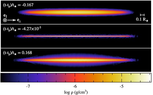
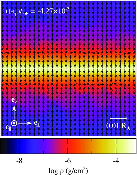
Snapshots showing the gas density along the transverse directions inside the stream element at different times (t − t_p)/t_⋆ = −0.167, −4.27 × 10⁻³, and 0.168, which are offset with respect to that t = t_p of pericentre passage and normalized by the stellar dynamical time-scale |$t_{\star }\approx 0.44 \, \rm h$|⁠. The value of the density increases from black to white, as shown on the colour bar. The white segment on the first snapshot indicates the scale used and the orientation is given by the white arrows. These snapshots are taken around the point where the gas reaches maximal collapse that results in a bounce, which reverses the infalling motion to make the gas expand after pericentre passage.

Open in new tabDownload slide

The hydrodynamics of the nozzle shock can be examined more precisely from Fig. 8, which displays the density (upper panel) and vertical velocity (lower panel) profiles along the vertical direction that are obtained at different times by dividing the gas within the stream element into slices parallel to the equatorial plane. The chronological ordering of the different curves is indicated schematically at the bottom of the upper panel. At (t − t_p)/t_⋆ = −0.65 (black solid line), the density is still uniform on the scale of |z| ≤ 0.015R_⋆, with a maximal value larger than initially as a result of compression during the infall phase. The velocity profile is also perfectly homologous due to the ballistic gas motion that is unaffected by small pressure forces. As matter gets closer to pericentre at (t − t_p)/t_⋆ = −0.066 (red dashed line) and −0.024 (blue long-dashed line), the central density starts rising while the gas gets decelerated by growing central pressure gradients, as can be seen from a steepening of the velocity profiles. The gas reaches its maximal density of |$\rho \approx 10^{-3} \, \rm g \, cm^{-3}$| for a range of vertical distances |z| ≲ 10⁻³R_⋆ at (t − t_p)/t_⋆ = −0.016 < 0 (orange dotted line), which is before pericentre passage as predicted in Section 2.3. At the same time, the collapse of the matter closest to the equatorial plane gets reverted by pressure forces as indicated by a change in sign of the vertical speeds. Additionally, a shock wave gets launched that propagates outward (coloured arrows) at later times (t − t_p)/t_⋆ = −0.0075 (purple dash–dotted line) and 0.00076 (green dash–dot–dotted line) through matter still collapsing at supersonic speeds. Gas entering this shocked region at increasing vertical heights has their infalling motion reversed, which continues until the shock wave has swept through the entire stream. This process is displayed in Fig. 9, which zooms in on the gas density near the centre of the stream shortly after the start of the nozzle shock at (t − t_p)/t_⋆ = −4.27 × 10⁻³. As seen from the black arrows that indicate the direction of the velocity field, matter near the equatorial plane undergoes expansion behind the shock wave, while the gas further away still moves inward. Following this bounce, the density drops back to its value before pericentre passage with a velocity profile that becomes homologous again, as seen in Fig. 8 at (t − t_p)/t_⋆ = 0.47 (brown dash–dash–dotted line). The hydrodynamics of this shock is similar to that taking place during deep tidal disruptions due to the strong compression of the star at pericentre (Guillochon et al. 2009; Brassart & Luminet 2010).

Figure 8.

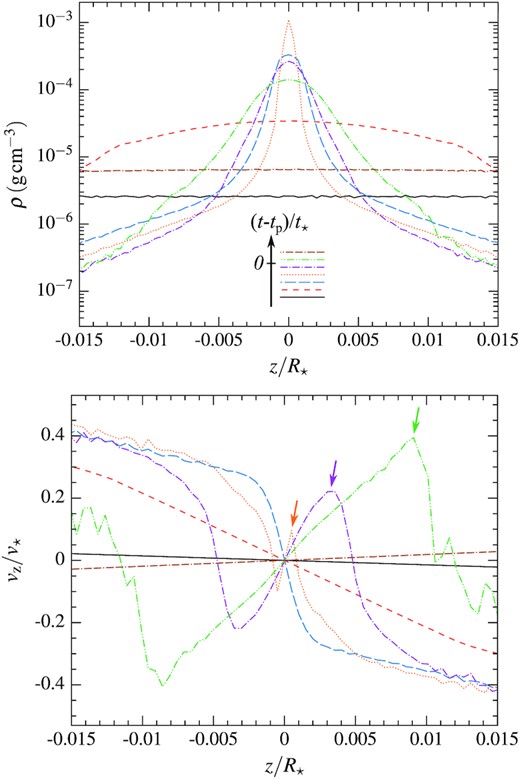
Density (upper panel) and vertical velocity (lower panel) profiles along the vertical direction at different times (t − t_p)/t_⋆ = −0.65 (black solid line), −0.066 (red dashed line), −0.024 (blue long-dashed line), −0.016 (orange dotted line), −0.0075 (purple dash–dotted line), 0.00076 (green dash–dot–dotted line), and 0.47 (brown dash–dash–dotted line). This chronological ordering of the different curves is indicated schematically at the bottom of the upper panel. The profiles are obtained by dividing the gas distribution into slices parallel to the equatorial plane. The coloured arrows in the lower panel indicate the position of the shock wave that vertically sweeps through the stream, reversing the direction of motion of the collapsing matter.

Open in new tabDownload slide

Figure 9.

Zoom-in on the centre of the stream element showing its density at (t − t_p)/t_⋆ = −4.27 × 10⁻³, with black arrows of the same length denoting the direction of the velocity field. The value of the density increases from black to white, as shown on the colour bar. The white segment indicates the scale used and the orientation is given by the white arrows. This snapshot is taken shortly after the start of the nozzle shock as the shock wave ahead of the expanding gas passes through matter still approaching the equatorial plane, which has the effect of reverting its direction of motion.

Open in new tabDownload slide

Fig. 10 shows the gas density (upper panel) and perpendicular velocity (lower panel) profiles along the in-plane direction at the same times as in Fig. 8. The gas density increases for |ξ| ≲ R_⋆, which is entirely due to the much stronger vertical compression. Because of low in-plane pressure gradients, the velocity profiles remain close to homologous at all times.⁹ In contrast with the vertical direction, these profiles get shallower as the stream element moves inward to reach v_⊥ ≈ 0 at pericentre since all the gas velocities are aligned with that of the centre of mass along the tangential direction. Later on, the velocities switch sign due to a divergence of the gas trajectories as the stream element moves away from the black hole.

Figure 10.

Density (upper panel) and perpendicular velocity (lower panel) profiles along the in-plane direction at the same times as used in Fig. 8. The chronological ordering of the different curves is indicated schematically at the bottom of the upper panel. The profiles are obtained by dividing the gas distribution into slices perpendicular to the equatorial plane.

Open in new tabDownload slide

The dissipation taking place during pericentre passage can be analysed from Fig. 11, which shows the evolution of the specific internal energy (upper panel) and the entropy (lower panel) normalized by its initial value. During the infalling phase, the compression experienced by the gas results in close to adiabatic heating at approximately constant entropy. Dissipation at the nozzle shock results in a sharp entropy jump close to pericentre associated with an increase of the internal energy by several orders of magnitude. The maximum value reached is |$u \approx 10^{-2} v^2_{\star }$| when averaging over the whole stream element (black solid line) and a factor of a few larger when considering only the hottest parts of the gas (red dashed line). The corresponding maximal temperature is of order |$T = m_{\rm p} u / k_{\rm B} \approx 10^5 \, \rm K$|⁠, which is high enough to ionize hydrogen, as we further explain in Section 4.8. As expected, the injected internal energy is similar to the kinetic energy of the infalling gas with vertical speeds v_z ≈ 0.3v_⋆ (see lower panel of Fig. 8). Just upstream from the shock, the Mach number is |$\mathcal {M} = v_{\rm z}/c_{\rm s} \approx 30 \gg 1$|⁠, using the sound speed c_s = (10u/9)^1/2 ≈ 0.01v_⋆ of the cold infalling gas. The magnitude of the entropy jump is consistent with that obtained from the jump conditions at a strong shock, which predicts an increase by a factor of |${\sim} (2\gamma / \gamma +1)(\gamma -1/\gamma +1)^{\gamma } \mathcal {M}^2 \approx 0.12 \, \mathcal {M}^2 \approx 100$| (equation 1.85 of Zel’dovich & Raizer 1967) for γ = 5/3. After the shock, the gas cools adiabatically through expansion that induces a fast decrease of the internal energy. Importantly, it however remains on average hotter than before pericentre due to the entropy jump.

Figure 11.

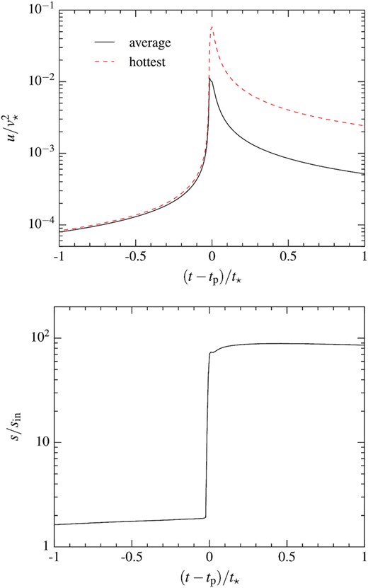
Evolution of the specific internal energy (upper panel) and entropy (lower panel) during the nozzle shock. The energy is obtained by averaging over the whole stream element (black solid line) and using only the |$10{{\ \rm per\ cent}}$| of particles with the largest energies (red dashed line). The entropy is computed as s = uρ^−2/3, which we normalize by its initial value. The time is offset with respect to that t = t_p of pericentre passage and normalized by the stellar dynamical time-scale |$t_{\star }\approx 0.44 \, \rm h$|⁠.

Open in new tabDownload slide

Because of their distinct locations with respect to the black hole, different parts of the stream element experience relative accelerations along the longitudinal direction that cause shearing motion. This effect can be analysed from Fig. 12 that shows the profile of the parallel velocity along the in-plane direction at different times. The chronological ordering of the different curves is indicated schematically in the lower right-hand corner. During the infalling phase at (t − t_p)/t_⋆ = −197 (black solid line), −1.5 (red dashed line), −0.92 (blue long-dashed line), and −0.34 (orange dotted line), the profiles progressively steepen as shearing becomes stronger due to the increase in relative acceleration across the stream element at lower radii. This trend continues until pericentre passage where the e_⊥ direction is radial and all the fluid elements have velocities tangential with respect to the black hole. At this point, the parallel speed can therefore be approximated as |$v_{\parallel } = \xi \mathop {}\!\mathrm{d}v / \mathop {}\!\mathrm{d}R \approx A_{\parallel } \xi v_{\rm p} / R_{\rm p}$| with A_∥ = 0.5 because all the gas inside the stream element is on close to parabolic orbits with v ∝ R^−1/2. Here, we have set the centre of mass velocity to its value v_c = v_p at pericentre. This analytical homologous profile (thick grey dashed line) coincides as expected with that obtained from the simulation closest to pericentre at (t − t_p)/t_⋆ = 0.00076 (purple dash–dotted line).¹⁰ Importantly, we find that the parallel speed is limited to v_∥ ≲ v_⋆ because of the relation v_p ≈ R_pv_⋆/R_⋆ at the tidal radius and the fact that the gas is confined to ξ ≲ R_⋆. After pericentre passage at (t − t_p)/t_⋆ = 0.55 (green dash–dot–dotted line) and 3.4 (brown dash–dash–dotted line), shearing weakens due to a decrease of the tidal force until the velocities becomes similar again across the stream element. However, note that the profile never reverses due to the rotation of the frame of reference that imposes the fluid elements with ξ > 0 to always remain closer to the black hole. As discussed in Section 4.6, shearing taking place near pericentre may lead to additional dissipation if the gas has a viscosity, which could increase the level of heating compared to that induced by the nozzle shock only.

Figure 12.

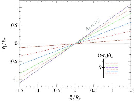
Parallel velocity profiles along the in-plane direction at different times (t − t_p)/t_⋆ = −197 (black solid line), −1.5 (red dashed line), −0.92 (blue long-dashed line), −0.34 (orange dotted line), 0.00076 (purple dash–dotted line), 0.55 (green dash–dot–dotted line), and 3.4 (brown dash–dash–dotted line). This chronological ordering of the different curves is indicated schematically in the lower right-hand corner. The profiles are obtained by dividing the gas distribution into slices perpendicular to the equatorial plane. The thick grey dashed line represents a homologous velocity profile evaluated from v_∥ = A_∥ξv_p/R_p with A_∥ = 0.5, where v_p denotes the centre of mass velocity at pericentre.

Open in new tabDownload slide

3.3 Recession to larger distances

We now turn our attention to the evolution of the stream element past pericentre to determine how its properties are affected by the passage through the nozzle shock. Fig. 13 displays the vertical (black solid line) and in-plane (red dashed line) widths as a function of distance from the black hole, which are computed from the simulation as the distances that contain half of the mass of the element. The dash–dotted lines of the same colours are obtained in the same way but switching off pressure forces in the simulation such that the gas moves on ballistic trajectories. Owing to the symmetry of the gas properties with respect to the equatorial plane, this situation is remarkably equivalent to an instantaneous sign reversal of the vertical gas velocities at the point where its trajectories intersect near pericentre. We also reproduce with dotted lines the stream widths for the previous infalling phase, which were already plotted in the upper panel of Fig. 5. At low radii R ≲ 10R_t, the different widths evolve approximately as H ∝ R^1/2 (grey segment) in both transverse directions that is the same scaling as during the infalling phase. Note however that the vertical component is a factor of a few lower for the hydrodynamical evolution. This means that the outgoing stream element is more concentrated than before pericentre passage, as we explain later. As the stream element moves to larger radii R ≳ 10R_t, the widths obtained from the hydrodynamical simulation (black solid and red dashed lines) start to significantly differ from those assuming ballistic motion (dash–dotted lines). If the gas moved ballistically, we find that it would undergo a vertical collapse followed shortly after by a strong in-plane compression. This is due to the two intersections of trajectories we identified in Section 2.3 that occur when the centre of mass reaches the blue long-dashed line and then the purple point in Fig. 4. These episodes of compression are not present in the hydrodynamical evolution, which implies that the gas motion departs from purely ballistic trajectories owing to a non-instantaneous influence of pressure.

Figure 13.

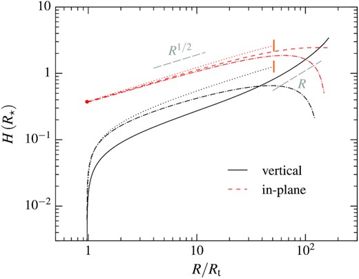
Vertical (black solid line) and in-plane (red dashed line) widths as a function of distance from the black hole as the stream element moves outward after pericentre passage (red circle). They are computed from the two-dimensional simulation as the distances from the centre of mass that enclose half of the mass in each direction. The dash–dotted lines of the same colours are obtained in the same way but setting pressure forces to zero in the simulation such that the gas moves ballistically. For ease of comparison, we also reproduce with dotted lines these widths for the previous infalling phase, which were already plotted in the upper panel of Fig. 5. The grey long-dashed segments indicate the scalings that the widths are analytically expected to follow in each phase.

Open in new tabDownload slide

To understand more precisely these deviations from ballistic motion, it is useful to determine how pressure forces modify the orbital parameters. Because of vertical pressure gradients, the outgoing gas undergoes a deflection of its velocity away from the equatorial plane. This induces a modification of its orbital plane whose intersection line with that of the centre of mass gets rotated along the direction of motion. This can be seen from the green dotted line displayed in Fig. 4 that represents this line computed when the centre of mass has reached the green point. Almost a full rotation of the intersection line is completed by this time compared to its initial location (blue long-dashed line). The intersection of trajectories predicted from ballistic motion is therefore prevented, which explains the absence of vertical collapse in our simulation. Another consequence is that the stream element moves perpendicularly to the rotated intersection line. As explained in Appendix  B, this causes the gas to expand faster in the vertical direction as seen from Fig. 13 at large radii where the scaling becomes close to H_z ∝ R (grey segment).

Although the pressure gradients are close to purely vertical immediately after the nozzle shock, the resulting bounce rapidly leads to a more circular transverse density distribution [see Fig. 6 at (t − t_p)/t_⋆ = 15.6].¹¹ As a result, pressure forces start additionally acting to make the stream expand along the in-plane direction. This causes the gas to get deflected away from the centre of mass trajectory, which induces a spread in the orientation of its different major axes with a range of precession angle ψ_h ≈ ±10⁻⁵|$\pi$|⁠. This influence of pressure can be directly seen by comparing the hydrodynamical (green dash–dotted line) and ballistic (blue dotted line) trajectories displayed in Fig. 4. While ballistic motion predicts an intersection with the centre of mass trajectory at the location of the purple point, this collision is prevented by the deflection induced by pressure forces. This provides an explanation for the absence of in-plane collapse in the hydrodynamical evolution, as we described before. As explained more in Appendix  C, an intersection is nevertheless still expected very close to apocentre. This can be seen from the flattening of the red dashed curve in Fig. 13 at the largest radii, which is expected to be followed by an in-plane compression. This type of interactions already predicted by Kochanek (1994) (see his fig. 5) may significantly affect the subsequent stream evolution, particularly by broadening its angular momentum distribution.

We have seen that the influence of pressure is not limited to the nozzle shock, but also affects the gas motion during most of its later evolution towards apocentre. This is because of the entropy jump that increases the gas internal energy past pericentre despite similar densities (see Fig. 11). As the gas moves away from the black hole, the ratio of tidal to pressure forces scales as F_t/F_p ≈ GM_hH²/(uR³) ∝ R^−5/3 like during the infalling phase since the stream properties evolve similarly as long as R ≲ 10R_t (see Fig. 13). However, the value of this ratio shortly after pericentre passage is of |$F_{\rm t}/F_{\rm p}|_{R\gtrsim R_{\rm p}} \approx 10$|⁠, which is more than an order of magnitude lower than before due to the entropy increase at the nozzle shock. Here, we have used |$u\approx 10^{-3} v^2_{\star }$| and H ≈ 0.1R_⋆ to get the numerical value, which corresponds to a time (t − t_p)/t_⋆ ≈ 1. As the stream moves outward, pressure forces can therefore become comparable to the tidal force, thus affecting the gas motion. A consequence is that self-gravity is not expected to become dynamically important again since it will likely be dominated by pressure forces even after the density has reached ρ ≳ ρ_sg near apocentre.¹²

The density profiles of the stream element are shown in Fig. 14 along the vertical (upper panel) and in-plane (lower panel) directions. They are obtained at different times (t − t_p)/t_⋆ = −1622 (grey dotted line), −197 (black solid line), −15.6 (red dashed line), 15.6 (blue long-dashed line), 197 (orange dotted line), and 1622 (purple dash–dotted line) that are also displayed in the snapshots of Fig. 6. The fact that these times have exactly opposite signs implies that the stream element is at the same distance from the black hole of R/R_t = 9.3, 51.2, and 158 on opposite sides with respect to pericentre passage. At the lowest two radii, the gas is more concentrated¹³ and features a more extended density profile along the vertical direction after pericentre passage than before. We suggest that this difference can be traced back to the bounce following the nozzle shock, during which the expansion of the gas closest to the equatorial plane is hampered by matter still moving inward (see Fig. 9). As a result, the outward motion of this central part of the stream is slowed down compared to matter near the boundary that expands instead in complete vacuum. At the largest radius close to apocentre, the central concentration is reduced while the gas gets more compressed along the in-plane direction than during the infalling phase, which is consistent with the widths evolution displayed Fig. 13 (solid black and red dashed line) at R ≳ 100R_t.

Figure 14.

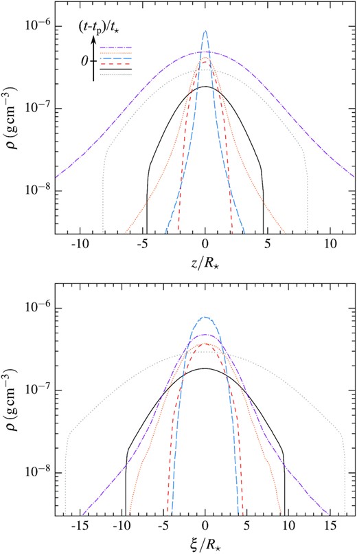
Density profiles along the vertical (upper panel) and in-plane directions (lower panel) at different times (t − t_p)/t_⋆ = −197 (black solid line), −15.6 (red dashed line), 15.6 (blue long-dashed line), 197 (orange dotted line), and 1622 (purple dash–dotted line) that are also shown in the snapshots of Fig. 6. The grey dotted line corresponds to (t − t_p)/t_⋆ = −1622 that is before the start of the two-dimensional simulation. It is obtained by extrapolating from the initial density profile at (t − t_p)/t_⋆ = −197 using the scaling H ∝ R^1/2 identified during the infalling phase for the transverse widths evolution based on the upper panel of Fig. 5 and the analytical evolution of the mass of the stream element given by equation (7). The chronological ordering of the different curves is indicated schematically in the top left-hand corner of the upper panel. The three earliest profiles are taken at times exactly opposite to those of the three latest ones, which means that they are obtained when the stream element is at the same distance from the black hole of R/R_t = 9.3, 51.2, and 158 before and after pericentre passage, respectively.

Open in new tabDownload slide

Apart from the above differences in the exact mass distribution within the stream element, we find that the density profiles of Fig. 14 are overall similar when considered at the same distance from the black hole. This is because the stream element does not undergo significant net expansion due to the impact of pressure forces at the nozzle shock and later in the evolution. This conclusion is also confirmed by the widths computed in Fig. 13 that only vary by a near-unity factor between the infalling phase and the recession towards apocentre. This qualitative evolution drastically differs from that obtained in several previous works, which find that the stream gets strongly inflated during pericentre passage.

4 DISCUSSION

4.1 Convergence study

We now carry out a convergence study to evaluate the dependence of the results on the resolution used. To this aim, we show in Fig. 15 the vertical (solid black line) and in-plane (red dashed line) widths as a function of number of particles used to describe the stream element. This number is successively set to N_p ≈ 2 × 10², 2 × 10³, 2 × 10⁴, and 2 × 10⁵, corresponding to the points of the same colours. The highest particle number is that used in the simulation presented throughout this paper. As before, the widths are defined by the distance from the centre of mass that contains half of the mass in each direction. Here, they are evaluated after the nozzle shock at a time (t − t_p)/t_⋆ = 197 when the gas has receded back to a distance R = 51.2R_t from the black hole. The widths are essentially identical at the largest particles numbers, which demonstrates that the results presented in the paper are not expected to change if resolution is further increased. At lower particle numbers, the stream becomes both thicker and more circular, which we attribute to an artificially weaker vertical compression at the nozzle shock that makes the bounce more isotropic.

Figure 15.

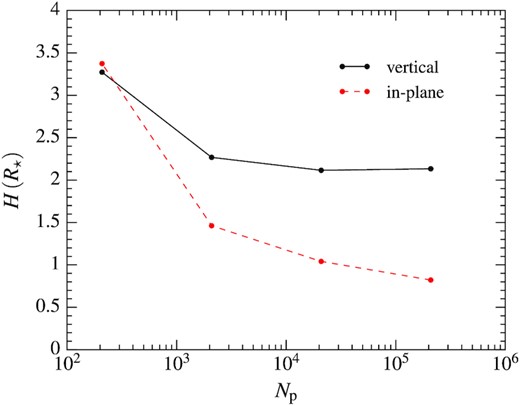
Vertical (black solid line) and in-plane (red dashed line) widths as a function of number of particles, successively set to N_p ≈ 2 × 10², 2 × 10³, 2 × 10⁴, and 2 × 10⁵ as displayed with the points of the same colours. These widths are defined as the distances from the centre of mass that enclose half of the mass in each direction. They are computed at a time (t − t_p)/t_⋆ = 197 when the stream element has receded back to a distance of R = 51.2R_t from the black hole after pericentre passage.

Open in new tabDownload slide

Another source of artefacts in three-dimensional simulations is due to the possibility that a fraction of the orbital kinetic energy gets artificially dissipated in addition to the much lower transverse component. Because of the large ratio of |$v^2_{\rm p}/v^2_{\rm z} \approx 10^4$| between these two energies, even a very small conversion of the orbital kinetic energy into heat can dramatically affect the transverse evolution. The important lack of resolution suffered by three-dimensional simulations near pericentre likely makes them prone to overestimating this energy transfer. This effect may accelerate the subsequent gas expansion, resulting in an artificially large width of the stream as it gets away from the black hole. This is indeed the qualitative trend seen in three-dimensional simulations carried out by early works (Lee & Kim 1996; Ayal et al. 2000) and more recent investigations at higher resolution. While these authors find that the outgoing stream reaches a thickness comparable to its distance from the black hole, our two-dimensional study predicts similar transverse widths before and after pericentre passage (see Fig. 14). We suggest that the above effects affecting three-dimensional simulations are at the origin of these differences.

4.2 Validity of the two-dimensional approach

Our two-dimensional simulation neglects the mutual interaction between successive stream elements and we check here the validity of this assumption. A first possibility is that the returning stream gets heated before passing through the nozzle shock due to pressure waves travelling upstream from matter already undergoing this interaction. The ratio of the sound speed c_s = (9u/10)^1/2 at which this signal travels to the orbital velocity v_p ≈ (2GM_h/R_p)^1/2 at pericentre is of about c_s/v_p ≈ 10⁻³ ≪ 1, making use of the internal energy |$u \approx 10^{-2} v^2_{\star }$| found near the nozzle shock (see Fig. 11). This implies that the shocked matter is unable to communicate with the upstream gas. A given section of stream therefore only starts experiencing significant heating when it arrives at the nozzle shock. Our neglect of this longitudinal energy transfer is therefore fully justified.

Longitudinal pressure gradients can also develop downstream from the nozzle shock, leading to the acceleration of highly compressed matter towards the already expanding gas along the direction of motion. To evaluate the importance of this effect, we calculate the longitudinal pressure force |$F_{\rm \, p \parallel } = -\nabla P \cdot \boldsymbol {e}_{\parallel }/\rho$| by estimating the gradient from the pressure variation of the stream element at successive times divided by the offset in position of its centre of mass. This leads to a maximal value of |$F_{\rm p \, \parallel } \approx 0.01 v^2_{\star }/R_{\star } \gt 0$| that is reached immediately downstream from the nozzle shock due a reduction in pressure. To determine its importance, this force must be compared to that in the vertical direction, which can be directly estimated from |$F_{\rm p ,z} \approx u/H_{\rm z} = 100 \, v^2_{\star }/R_{\star }$|⁠. Here, we have used the gas properties found in the simulation when the gas is vertically compressed to a small width H_z ≈ 10⁻³R_⋆ (see upper panel of Fig. 5). We therefore find that the longitudinal component of the pressure force is much lower than in the vertical direction with a ratio |$F_{\rm p \, \parallel } / F_{\rm \, p ,z} \approx 10^{-4} \ll 1$|⁠. Its influence on the dynamics can then be neglected as assumed in our two-dimensional approach.^14,15

4.3 Extrapolation to other parameters

We now evaluate the dependence of our results on the choice of parameters. The strength of the nozzle shock can be estimated from the vertical component of the stream velocity near pericentre where the trajectories would intersect in the ballistic limit. This speed is approximately given by |$v^{\rm max}_{\rm z} \approx v_{\rm p} \vartheta$| where ϑ denotes the inclination angle between the orbital plane of the collapsing gas and that of the stream centre of mass. As explained in Section 2.3, gas motion becomes close to ballistic from the moment when the tidal force starts dominating the dynamics. For the stream element we considered, this occurs shortly after apocentre passage, which we argue remains valid in general due to the sharp decrease in density experienced by the gas as it starts moving inward (see lower panel of Fig. 5). Therefore, hydrostatic equilibrium is maintained down to a distance larger than the semimajor axis, i.e. R_eq  ≳ a. The inclination angle is then given by the ratio of the average stream width to its distance from the intersection line at this location, i.e. ϑ ≈ tan ϑ = H_eq /d_eq. This distance can be geometrically expressed as d_eq = ((R_pR_a)/(2a/R_eq  − 1))^1/2, where R_a ≈ 2a denotes the apocentre distance. Making use of R_eq  ≳ a yields d_eq  ≳ b ≈ (R_pa)^1/2 that is comparable to the semiminor axis b = (R_pR_a)^1/2 of the stream element, as can also be seen from Fig. 4 for our parameters. The stream width at this location is estimated from H_eq  ≈ H_t(R_eq /R_t)^1/2 ≈ H_t(a/R_p)^1/2β^−1/2 according to the scaling followed shortly after stellar disruption, introducing the normalization H_t ≈ 0.1R_⋆.

The specific stream element followed in our simulation is mostly chosen for numerical convenience (see Section 2.1). We find that its initial vertical velocity profile is close to homologous, although this may change for other parts of the stream. Deviations from homology can come from oscillations around hydrostatic equilibrium close to the moment when the tidal force overwhelms self-gravity. It may also be due to a transverse density profile that significantly differs from the binormal distribution we use. Such a difference is visible for the most bound tip of the returning gas that features a dense core offset with respect to more tenuous surrounding matter. As discussed by Stone et al. (2013) in the context of deep stellar disruptions, non-homologous compression implies that gas at initially different vertical distances reaches the equatorial plane at distinct locations along the trajectory. This desynchronization may cause fluid elements to cross each other multiple times away from the stellar orbital plane, leading to internal collisions. This implies that the energy dissipation at the nozzle shock could be more gradual than found in our simulation where this interaction is confined to a small region. We argue that this can lead to a more isotropic bounce compared to the gas motion we predict that is largely limited to the vertical direction.

The stream element considered initially has a range of pericentre distances that causes its in-plane width to remain H_⊥ ≳ R_⋆ during the nozzle shock (see Fig. 13). Physically, this is due to a spread in angular momentum imparted by pressure forces during the previous evolution of the stream around hydrostatic equilibrium. However, this in-plane width would be reduced for the parts of the stream entirely dominated by the tidal force since their prior evolution occurs at constant angular momentum. This effect may result in more in-plane compression or even crossing of trajectories along this direction. The nozzle shock could therefore become more isotropic with a larger amount of gas being significantly deflected along the equatorial plane than what our simulation predicts. Settling these uncertainties would require to improve our understanding of the orbital properties of the different parts of the returning stream including its small angular momentum, which we defer to the future.

4.4 Role of relativistic effects

4.5 Consequences on the self-crossing shock

This self-crossing shock efficiency is shown in Fig. 16 with the black solid line as a function of the intersection radius that ranges from near pericentre (circles) to apocentre (squares). It additionally assumes that the black hole is non-rotating with a_h = 0 such that the centre of mass of the two streams evolve on the same orbital plane. The grey vertical dotted line indicates the value R_int = 118R_t corresponding to our choice of parameters. We find that η_sc ≈ 0.9 at all distances, with the small reduction compared to unity coming from the fact that the stream element is more centrally concentrated after pericentre passage than before. Its central density is larger by a factor of ρ_out(0)/ρ_in(0) ≈ 2 (upper panel of Fig. 14) that explains the value of the efficiency found.²¹ We therefore conclude that the self-crossing shock remains very efficient despite the modifications induced by the nozzle shock, which results for the low level of net stream expansion it induces.

Figure 16.

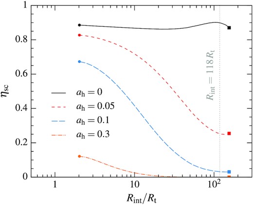
Efficiency of the self-crossing shock obtained from equation (17) as a function of the intersection radius where this collision occurs for different black hole spin parameters a_h = 0 (black solid line), 0.05 (red dashed line), 0.1 (blue long-dashed line), and 0.3 (orange dash–dotted line). The vertical grey dotted line indicates the location of the intersection radius R_int = 118R_t resulting from apsidal precession for the orbital parameters of the stream element considered.

Open in new tabDownload slide

A more quantitative evaluation of this impact of black hole spin can be done by computing the self-crossing shock efficiency from equation (17), introducing the vertical offset of equation (18) between the centres of the two colliding stream components. This efficiency is shown in Fig. 16 for several spin parameters, assuming γ = |$\pi$|/2 and sin i = 1 for simplicity. For a_h = 0.05 (red dashed line), we find that the efficiency is strongly reduced to η_sc ≲ 0.5 for an intersection radius R_int ≳ 50R_t, as predicted by equation (20). The self-crossing shock is almost as efficient as for a_h = 0 (black solid line) with η_sc ≳ 0.8 close to pericentre due to the reduced impact of the sublinear width increase. Increasing the black hole spin to a_h = 0.1 (blue long-dashed line) further decreases the efficiency but with a similar rise at low radii. For a_h = 0.3 (orange dash–dotted line), the self-crossing shock is inefficient at all radii with η_sc ≲ 0.1 because most of the gas misses the collision due to a large vertical offset.

The above calculations suggest that the self-crossing shock is efficient with η_sc ≳ 0.9 as long as the black hole has a negligible spin. This conclusion lends support to the assumption of identical stream components used in local simulations of this interaction (Lee et al. 1996; Kim et al. 1999; Jiang et al. 2016; Lu & Bonnerot 2020). In this situation, the shocked gas is launched into a large-scale quasi-spherical outflow that can have a significant unbound fraction. When the bound matter returns near the black hole, an accretion disc may promptly form with a direction of rotation potentially opposite to that of the original star (Bonnerot & Lu 2020; Bonnerot, Lu & Hopkins 2021).²⁵ If the efficiency is reduced to η_sc ≳ 0.1, the interaction likely produces a non-spherical outflow that contains less unbound matter. Nevertheless, we still expect a significant amount of gas to have their trajectories deflected that could initiate the formation of an accretion disc. In the future, we intend to better characterize the outcome of the self-crossing shock if the collision is significantly offset.

If the efficiency is η_sc ≪ 1, most of the stream components miss each other on the first pass. In this situation, the stream continues to evolve on a largely unaffected trajectory for several orbital periods until a delayed collision eventually occurs (Guillochon & Ramirez-Ruiz 2015). Similarly to the nozzle shock, we expect the stream to experience several episodes of strong compression that may lead to additional dissipation. Studying this stage of evolution is necessary to precisely determine the time of the first intersection and the properties of the stream components involved. This could be achieved through a generalization of the two-dimensional approach presented here, which we intend to do in the future.

4.6 Impact of viscous dissipation

To estimate the value of the viscosity, we make use of the prescription ν = αc_sH_z, involving the local sound speed and vertical extent of the stream. At pericentre, this estimate leads to ν_p/(R_⋆v_⋆) ≈ 10⁻⁵(α/0.1)(u/10⁻²v_⋆)^1/2(H_z/10⁻³R_⋆), setting the internal energy and stream vertical width to their values at the nozzle shock, and the viscosity parameter to α ≈ 0.1. The obtained viscosity is ν_p/R_⋆v_⋆ ≈ 10⁻⁵ ≪ 10⁻², implying that the resulting heating rate of equation (21) is much lower than that due to the shock. The magnetorotational instability (MRI; Balbus & Hawley 1991) could provide a physical source of viscosity after saturation has been reached. However, this requires several orbital periods while in our situation the stream remains near pericentre for only about half an orbit (Guillochon et al. 2014; Chan, Krolik & Piran 2018). For this reason, saturation is unlikely to be attained that may strongly reduce the viscosity compared to the above value based on α ≈ 0.1. An improved evaluation of this effect would require to carry out a dedicated magnetohydrodynamical simulation of the stream passage at pericentre.

4.7 Influence of magnetic fields

4.8 Effect of radiative processes

As it passes through the nozzle shock, the hydrogen that had recombined during the previous evolution (e.g. Kasen & Ramirez-Ruiz 2010) gets reionized due to the large temperatures reached. This however does not affect the hydrodynamics of the interaction since the specific energy required for ionization is |$E_{\rm H}/m_{\rm p} \approx 5 \times 10^{-4} v^2_{\star }$| where |$E_{\rm H} = 13.6 \, \rm eV$|⁠, which is much lower than that |$u \approx 10^{-2} v^2_{\star }$| injected due to dissipation. As the gas expands at larger distances, its temperature decreases back to |$T \lesssim 10^4 \, \rm K$| such that hydrogen recombines again, which is associated with a jump in entropy. This effect may result in additional expansion compared to what our adiabatic simulation predicts, if radiative cooling can be neglected.

5 SUMMARY

We have carried out the first dedicated study of the return of the debris stream towards the black hole following a stellar disruption. This is realized by first performing a three-dimensional simulation of the disruption, from which we obtain the hydrodynamical properties of a given section of stream. These properties are then used to initialize a two-dimensional simulation that follows the subsequent transverse evolution of this stream element in the frame comoving with its ballistic centre of mass and corotating with the longitudinal direction. Using this numerical technique, we are able to study with sufficient numerical resolution the approach of this gas towards the black hole, its passage at pericentre where the nozzle shock takes place, and its recession back to large distances. The results of this investigation and the main points of the accompanying discussion can be summarized as follows.

• During its infall towards the black hole, the transverse widths of the stream element decrease approximately as H ∝ R^1/2, which is specified by the dominant tidal force. Because of a combination of this homologous compression and longitudinal stretching, its density increases according to ρ ∝ R^−1/2 (see Fig. 5).

• When it gets close to the black hole, the stream is strongly compressed along the vertical direction due to an intersection of its different orbital planes. Its vertical width sharply decreases down to H_z ≈ 10⁻³R_⋆, while its in-plane extent remains of H_⊥ ≈ 0.1R_⋆. This point of maximal compression is reached slightly before pericentre, as predicted from ballistic motion.

• The strong compression near pericentre results in the formation of the nozzle shock that dissipates the kinetic energy associated with vertical motion. As a result, a shock wave is launched from the equatorial plane that rapidly sweeps through the collapsing gas. The infalling motion of this matter is reverted, which makes it bounce back to larger vertical distances.

• While the rest of its evolution is entirely adiabatic, the gas undergoes a sharp increase of its specific internal energy to a maximal value of |$u \approx 0.1 v^2_{\star }$| during the nozzle shock (see Fig. 11). This dissipation is associated with an entropy jump by about two orders of magnitude, causing an overall increase of pressure forces that therefore become important at later times.

• Throughout its evolution, the stream element experiences shearing along its longitudinal direction due to the relative acceleration between its parts located at different distances from the black hole. This effect is the strongest at pericentre where the shearing profile becomes close to that expected from a Newtonian circular flow.

• After pericentre passage, the gas expands with transverse widths increasing as H ∝ R^1/2 close to the black hole. At larger distances, in-plane expansion stalls to eventually result in a collapse near apocentre while the vertical width increases faster as H_z ∝ R (see Fig. 13). Contrary to the infalling phase, the gas evolution significantly deviates from ballistic motion due to the influence of pressure forces.

• The nozzle shock does not result in significant net expansion of the gas during pericentre passage, but rather modifies its transverse density profile. The outgoing stream element is slightly more centrally concentrated with a larger extent than when it was at the same distance from the black hole before pericentre passage.

• Numerical convergence is reached for a particle number |$N^{\rm 2D}_{\rm p} \approx 10^5$| used to describe the stream element in our two-dimensional approach (see Fig. 15). We estimate that resolving the nozzle shock within a three-dimensional simulation of stellar disruption would require |$N^{\rm 3D}_{\rm p} \approx 10^{14}$| particles, which does not appear computationally feasible.

• Our simulation finds that the stream element has a lower vertical width that increases slower with radius than previously assumed. This implies that relativistic nodal precession may be able to prevent the self-crossing shock induced by apsidal precession even for slowly spinning black holes with a_h ≳ 0.1 (see Fig. 16).

• If the stream is magnetized, the nozzle shock can be affected by the additional support from magnetic pressure against vertical collapse. We estimate that this effect becomes important for stellar magnetic field strength along the direction of stream elongation of about |$B_{\parallel \star } \gtrsim 400 \, \rm G$|⁠, which may be reached for solar-type stars.

ACKNOWLEDGEMENTS

We thank Roseanne Cheng, Phil Hopkins, Chris Matzner, Ramesh Narayan, Martin Pessah, Sterl Phinney, and Tony Piro for useful discussions. We acknowledge the use of splash (Price 2007) for producing most of the figures in this paper. This research benefited from interactions at the ZTF Theory Network Meeting, partly funded by the National Science Foundation under Grant No. NSF PHY-1748958. The research of CB was funded by the Gordon and Betty Moore Foundation through Grant GBMF5076. This project has received funding from the European Union’s Horizon 2020 Framework Programme under the Marie Sklodowska-Curie grant agreement no. 836751. WL was supported by the David and Ellen Lee Fellowship at Caltech and the Lyman Spitzer, Jr Postdoctoral Fellowship at Princeton University. The authors thank the Yukawa Institute for Theoretical Physics at Kyoto University, where this work was initiated during the YITP-T-19-07 International Molecule-type Workshop ‘Tidal Disruption Events: General Relativistic Transients’. CB is particularly grateful to Richard D. Saxton for recognizing the knotty problem of the nozzle shock at this conference.

DATA AVAILABILITY

The data underlying this paper will be shared on reasonable request to the corresponding author. A public version of the gizmo code is available at http://www.tapir.caltech.edu/~phopkins/Site/GIZMO.html.

Footnotes

REFERENCES

APPENDIX A: EQUATIONS OF MOTION

APPENDIX B: WIDTH SCALING

To apply this result to the infalling phase of the stream element, the most convenient choice is to set the initial conditions at the moment when the tidal force starts dominating self-gravity. Because the gas is still close to hydrostatic equilibrium, the transverse velocities are almost zero, i.e. A_{z, in} = A_{z, eq}  ≈ 0³⁰ at a distance R_in = R_eq from the black hole. This implies that q ≈ 0 in equation (B2) such that both transverse widths are expected to reach the scaling H ∝ R^1/2 slightly later when the gas has moved inward to R ≲ R_eq, as we indeed find in the hydrodynamical simulation we carried out (see upper panel of Fig. 5). Note that the two scalings identified above can also be qualitatively understood for the vertical width in terms of motion relative to the line where the different orbital planes of the stream element intersect. If its centre of mass moves almost parallel to this line like in the infalling phase, the scaling is expected to be parabolic as we just found. Motion orthogonal to this line results instead in a linear scaling with H_z ∝ R, which agrees with the evolution after pericentre passage when the gas reaches large radii (see Fig. 13) due to the rotation of the intersection line from the blue long-dashed line to the green dotted one in Fig. 4.

APPENDIX C: ORBIT INTERSECTIONS

The gas inside the stream element evolves on different orbital planes that are inclined with respect to that of its centre of mass. These planes intersect along the same line if the transverse velocity profile is homologous, either corresponding to compression or expansion. We find this description to be a good approximation, but deviations from a homologous profile are possible (see Section 4.3), which would cause the orbital planes to intersect at distinct locations along the trajectory in a desynchronized way (Stone et al. 2013). The orbital plane intersection line is parallel to the centre of mass velocity at the location where the gas experiences no transverse motion. This is because the vertical extent of the stream is then maximized, implying that its centre of mass has reached the largest possible distance from the intersection line where its velocity is necessarily tangential. For the returning debris stream, this condition is satisfied at R = R_eq when the tidal force starts to become dominant because the gas is close to hydrostatic equilibrium. As long as R_eq  ≥ a, the orientation of the centre of mass velocity at this location implies that the stream collapses vertically slightly before pericentre passage (see Fig. 4). We emphasize that this conclusion does not hold for the similar process of strong stellar compression where this collapse generally occurs after pericentre passage (Luminet & Marck 1985). This difference stems from the fact that the star follows a parabolic orbit instead of an elliptic one for the bound debris. The equilibrium condition is in this case attained at the tidal radius where the centre of mass velocity is always oriented such that the parallel intersection line crosses the trajectory past pericentre.³¹

The different trajectories of the stream element may also intersect with that of the centre of mass along the equatorial plane, which results in an in-plane collapse of this gas. In his pioneering work, Kochanek (1994) claims that such intersections occur if the eccentricity satisfies e > 7 − 4q (given in the text of his section 3.2) where the parameter q specifies the slope of the angular frequency profile that can be written as q = A_∥ + 1 using our notation. We find that this condition can be obtained by imposing that gas with an offset ξ = ξ_p > 0 at pericentre has an apocentre distance larger than that of the centre of mass, which indeed causes the two trajectories to cross. This can be proved by showing that the relative variation in apocentre distance is given by ΔR_a/R_a = (ξ_p/R_p)(2(2A_∥ − 1)/(1 − e) − 1), so that ΔR_a/R_a > 0 yields e > 3 − 4A_∥ = 7 − 4q, as stated above. This condition appears to be marginally satisfied in our situation because the homology factor reaches at pericentre a maximal value of A_∥ ≳ (3 − e)/4 ≈ 0.5025 (see Fig. 12) using the eccentricity e ≈ 0.99 of the stream element. This confirms that ballistic trajectories are expected to intersect along the equatorial plane, which occurs at the purple point in Fig. 4. In addition to the difference in apocentre distances, we note that the precise location of this collision is affected by a small spread in apsidal angle ψ_i ≈ ∓10⁻⁵|$\pi$| between the ballistic trajectories imposed by the initial conditions that tends to make them converge past pericentre. As explained in Section 3.3, the gas gets deflected by pressure forces that instead causes a divergence of these outgoing trajectories, additionally enhanced by differential apsidal precession (see Section 4.4). Nevertheless, these small modifications do not prevent the in-plane collapse but merely pushes its location even closer to apocentre.