


ABSTRACT
We introduce a Fourier method (Fm) for the determination of best focus for telescopes with stars. Our method fits a power function, that we will derive in this paper, to a set of images taken as a function of focuser position. The best focus position is where the power is maximum. Fm was first tested with small refractor and Schmidt–Cassegrain telescopes. After the successful small telescope tests, we then tested Fm with a 2 m Ritchey–Chrétien–Coudé. Our tests show that Fm is immune to the problems inherent in the popular half-flux diameter method.
1 INTRODUCTION
One very important aspect in the collection of good astronomical data is the quality of the focusing of a telescope. A typical observing session can last between 1 and 12 h depending on the season and latitude. During this time, the ambient temperature will fluctuate. Temperature changes induce strain in optical components and the materials of the optical train from which a telescope is built and this can affect the focal point of the telescope. As a result, the position of the camera sensor connected at the end of the telescope has to be adjusted along with the temperature changes. To solve this problem, multiple focusing runs are done throughout the observing session to keep the images sharp. Without good and precise focusing, the collected data can be less than optimum for the given atmospheric conditions.
A quick survey of commercial and free autofocus programs (for example, focusmax, sgp, sharpcap)1 will show that the method that is employed by all these focusing programs is the half-flux diameter method (HFDm) or its predecessor.2 As the telescope gets into focus, the HFD measured for one single star or the average HFD from a star field decreases, and as the telescope gets out of focus, the HFD increases. Thus, the minimum of the HFD is the focus position. In principle, although the calculation of HFD is trivial, there are a few weaknesses with focusing using HFDm. We will highlight them throughout this paper and in Section 8.
In this paper, we will derive first the model used by the Fourier method (Fm) and then apply Fm to determine the focus of several telescopes. We start by applying Fm to two small refractors and one Schmidt–Cassegrain telescope (SCT). After the successful small telescope tests, we tested Fm with the 2 m Ritchey–Chrétien–Coudé (RCC) telescope installed in the Rozhen National Astronomical Observatory (Rozhen NAO) in Bulgaria.3 In all cases, we will compare the Fm focus results to the HFDm focus results.
We want to note that we are not the first who use Fourier space for autofocus purposes, for example, Bueno-Ibarra, Álvarez Borrego & Leonardo (2004). Additionally, we are also not the first authors who use autofocus methods in astronomy that do not rely on the detection of individual stars, for example, see the review by Popowicz et al. (2017). However, all previous approaches only show that there is some focus function that attains a special point (e.g. a global maximum) at focus. Those methods can only select the sharpest image from a series of images because the precise form of the focus function for a given image type is not known. In contrast, the novelty of our paper is that we compute the explicit form of the focus function for an image type that is very common in astronomy, namely images that contain stars. We will show that we can use our focus function to compute the focus position with a curve fit from a few defocused images. Our real world examples will also show that as long as there are stars in the image, our focus function is not sensitive to the presence of additional diffuse structures that may come from nebulae or galaxies. Fm is also insensitive to telescope designs that have obstructions in the light path from a secondary mirror. Furthermore, we will demonstrate a curve fitting algorithm that employs methods of robust statistics, that considerably reduces the influence of any remaining seeing problems and optical errors in the images. Finally, we will use our algorithm in connection with different statistical estimators to prove that Fm yields better results than the commonly used HFDm.
2 BASIC IDEA OF THE FOURIER METHOD

These two plots show the well-known feature that when the Gaussian is thin in real space, it is wide in Fourier space. The dashed horizontal line in real space space will be used for our discussion in Section 6.
We notice that, unlike HFDm that gets smaller as the focus is reached, Fm gets larger as the focal point is reached. By integrating under the curve in Fourier space, which is in effect low pass filtering, means that Fm is less noisy by design.
3 GAUSSIAN STAR FIELDS
We will assume that the exposure times at which the measurements for focusing are taken are long enough, so that on average, the intensity profiles of the stars can be described approximately by a Gaussian, i.e. we will ignore the transfer function of the telescope or we can think of this approximation as the consideration of the central peak of the PSF (point spread function) only. By making the Gaussian approximation, we will be able to compute a curve for the intensity profile of a star field in Fourier space.
Later, in Section 5, we will show that 4–8 s exposures are sufficient for telescopes of varying focal lengths and F-numbers to minimize any star shape variations from Gaussian that are due to atmospherics. Any remaining deviations can be handled by our outlier removal procedures with robust statistics.
3.1 Projection on to ωx-axis
3.2 Phenomenological model
3.3 Fm formula
3.4 Dense star field
In this paper, although we will be applying the sparse star field approximation to all of our examples in Section 5, we will digress here and consider the effects of a dense star field.
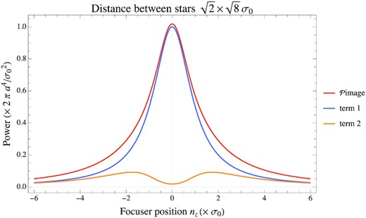
This is an example of the effect of the double sum of equation (16) when we have two stars spaced |$\sqrt{8}\bar{\sigma }_0$| in both the x and y directions. The double sum (term 2) clearly shows the dip in its value at focus. However, after adding in term 1, the result does not have a dip.
4 FITTING AND OUTLIER REMOVAL
A common method for curve fitting to data that approximately fulfills a known differentiable function is the Levenberg–Marquardt (LM) algorithm (Levenberg 1944; Marquardt 1963). This algorithm computes the sum of the squares of the residuals, i.e. the sum of the squared difference of a given function and the data. The algorithm proceeds as an iterative procedure searching for a local minimum of this residual. Unfortunately, because the iterative procedure only searches for a local minimum, the LM algorithm is known to depend on the precise choice of the initial data. In our case, we often have considerable outliers that come from seeing and high altitude clouds. These outliers make it difficult to start the LM algorithm with the required initial guess of the focuser position.
If we insert |$(\bar{\sigma }_0+\Delta \sigma)^2$| into equation (16) and consider |$\bar{\cal {P}}_{\rm image}(\Delta \sigma)\equiv \bar{\cal {P}}_{\rm image}((\bar{\sigma }_0+\Delta \sigma)^2)$| as a function of Δσ, we observe that both term 1 of equation (16) and |$\bar{\cal {P}}_{\rm image}(\Delta \sigma)$| have their maximum when Δσ = 0. Furthermore, when we compare |$\bar{\cal P}_{\rm image}$| of equation (16) to term 1, |$\bar{\cal P}_{\rm image}$| has a higher peak and tails. Therefore, we can can start with an initial fit with just term 1. For all of our examples, the fitting of just term 1 turns out to be sufficient for determining the focus position.
In equation (17), we have subtracted the parameter β. In the practical implementation, we get β from the magnitudes of the columns that represent white noise in the Fourier transformed image data. After β is subtracted from the magnitudes of the Fourier data, the remaining positive magnitudes are then summed. This also implies that the result of our procedure is generally different than what can be achieved by a simple summation of the magnitudes of the image’s pixels in real space. The Fm is distinctive in that it allows us to easily and quickly remove most of the noise. Without the ability to easily subtract the β term from the Fourier data, we would have to use the LM algorithm on |$\bar{\cal P}_{\rm Fm}(\zeta ;\alpha ,\beta ,\gamma)$|. However, we have no information about reasonable initial values for ζ, α, β, γ and thus the outcomes of the LM algorithm would not be reliable. It is only with the removal of β from |$\bar{\cal P}_{\rm Fm}(\zeta ;\alpha ,\beta ,\gamma)$|, that we can use powerful linear regression methods on Y(ζ, α, γ) that do not depend as much on the chosen initial values for ζ, α, γ when compared to the LM algorithm. In Section 4.1, we will use the LM algorithm only as a second stage to account for exponential functions in the double sums of equation (11). The LM algorithm is then used with initial values that we have acquired from the linear regression.
We expect that Y(ζ, α, γ) only resembles a parabola close to the focus position, because there are small corrections from the double sum in equation (11). It is therefore not surprising that we have found, in practice, that linear regression alone is insufficient for obtaining z0 from a fit of Y(ζ, α, γ) because we have to remove the outliers in the data. See the examples in Figs 3–5.
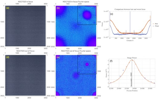
The images of NGC 7023 (Iris Nebula) taken by our refractor I. The (a) in-focus and (d) out-of-focus images in real space are both lightly stretched. The nebula can actually be seen in our 8 s exposure. After applying a 2D FFT to the real images, we obtain (b) and (e), which show that there are clear differences in the size of the lobes. The insets of (b) and (e) contain the same Fourier data except that zero frequency is at the centre rather than at the corners. (c) The projection of the lobes into 1D space is compared with a vertical logarithmic scale. (f) And when plotted as a function of focuser position and fitted to equation (15) tells us where the focus position is. The blue unfilled circles are the outliers identified by the fitting algorithm and ignored by the fit.
In order to fit our data appropriately and remove the remaining outliers from our rather small set of measurement points, we will use a modified version of a RANSAC algorithm (see Fischler & Bolles 1981 for the original description of RANSAC) that works deterministically and uses robust estimators (Schulz 2021) to solve the least trimmed squares problem (see Rousseeuw & Leroy 1987). We will describe this algorithm in detail below.
At this point, we have completed our work with the point set |${\cal A}_\ell$|. We restart this procedure with another selection of n points from |$\cal M$|. The above procedure is repeated until we have exhausted all |$N_{\cal M} \choose n$| combinations. We are then left with sets |${\cal A}_\ell$|, for |$\ell =1,\ldots ,{N_{\cal M} \choose n}$|, each having |$N_{{\cal A}_{\ell }}\ge n$| points |$\left(z_{\ell _j}, Y_{\ell _j} \right)$| for |$j=1,\ldots ,N_{{\cal A}_\ell }$|, because additional inliers may have been added to the initial combinations.
In order to increase the speed of the algorithm, we remove point sets |${\cal A}_\ell$| that are duplicates. We do this by associating a hash-value to each set |${\cal A}_\ell$|. Then, we can generate a hash table where we can look them up with a fast process to check whether there are equal hash-values, i.e. duplicate |${\cal A}_\ell$|’s. If found, the duplicates are marked and ignored. In order to save memory, the hash table may have to be cleared from time to time.
Finally, we perform simple linear regressions on each of the remaining point sets, |${\cal A}_\ell$|, for |$\ell =1,\ldots ,J \le {N_{\cal M}\choose n}$|, after duplicates have been removed, by using equation (19) again. The reduced χ2 error is calculated for each |${\cal A}_\ell$| using equation (20) but with |$n\rightarrow N_{{\cal A}_\ell }$|. At the end of the process, the algorithm returns the ‘found’ focus position, z0, to be the value that has the smallest |$\chi _{{\cal A}_\ell }^2$| from the point sets |${\cal A}_1,\ldots ,{\cal A}_J$|.
We can increase the speed of the algorithm tremendously by using parallel processing techniques (for example with OpenMP or by using the new parallelism features in the c++17 standard). We notice that this algorithm has its worst performance when |$n=N_{\cal M}/2$|, because |$N_{\cal M} \choose n$| is at its maximum here which leads to the largest possible number of attempted fits for a given data set. For example, a personal computer equipped with a Ryzen 9 3900X 12 core processor can robustly fit models with |$N_{\cal M}=24$| data points and |$n=N_{\cal M}/2=12$| using this algorithm in 3.17 s. We can increase the speed of the procedure further by using faster algorithms for the S-estimator by Croux & Rousseeuw (1992).
4.1 Introduction of a shaping term
We can then use the same statistical estimators as before in order to test, whether the points that were computed to be outliers with respect to initial parabola fit are still outliers when we use the LM algorithm with the shaping term. In general, the shaping term is a small correction to |$\bar{\cal P}_{\rm Fm}$|. We have found that when this correction is included in the fit, the resulting curve has a smaller fit error and a lower number of outliers. This has been confirmed by our experiments.
In Section 3.3, we have subtracted the parameter β from |$\bar{\cal P}_{\rm Fm}$|. β was determined by analysing the white noise of the images in Fourier space. While our experiments show that doing this is sufficient for determining the focus position within the critical focus zone (CFZ) (Sidgwick 1980), we can improve the fit with LM with small corrections to this value of β. We start the process with the initial correction value δβ = 0. Our experiments show that this reduces the fit error and the number of outliers of the curve fit even more.
For the practical implementation, we have used the improvements of the LM algorithm described in Transtrum & Sethna (2012).
4.2 Large data sets
Obviously, the algorithm is different from the solution of the trimmed least-squares problem. The values α(j) and γ(j) are now computed from a fit of all the points and the outliers only have a small influence on the result for the estimated focus position. Therefore, large errors that can be introduced by outliers do not lead to a wrong estimate of the minimum of the parabola anymore. Our tests with the 50 point samples (discussed in Section 7) show that this approach is sufficient for large sets of measurement data. Since the computation still depends in some way on all points that were measured, a second stage fit with the LM that includes the shape term and small corrections of β is especially beneficial to this method.
4.3 Comparison of fitting ease between Fm and HFDm
In order to compare HFDm to Fm, we have adapted the application from Schulz (2021) to provide fits and outlier rejection for data that is modelled by equation (17). The application in Schulz (2021) makes several fits where various estimators are used within the RANSAC inspired algorithm. This is done by replacing the S-estimator in equation (22) appropriately. The various estimators used in Schulz (2021) have different properties that can be described by an influence function. The latter determines the rate at which an estimate changes after the insertion of an outlier. The influence function of a robust estimator should be bounded because only then will large outliers not have an impact at all. More precisely, it can be characterized by the following properties:
Efficacy e*: The loss of efficacy of the estimator with respect to asymptotic variance. A high efficacy yields good estimates when the distribution of the samples is unknown.
Breakdown point ϵ*: This is the maximum percentage of points to have limited results on the estimate.
Gross error sensitivity γ*: This describes the worst influence of a small amount of contamination of fixed size.
Rejection point ρ*: The distance from a point to an estimate where the influence function vanishes. An infinite rejection point means that all points are considered, whereas a small rejection point means that large outliers do not contribute to the estimate. For example, if we use the S-estimator, we can calculate TU from equation (22) for a given data point. We will reject it if TU > τ where τ ∈ [2.5, 3] is some pre-defined tolerance.
We have used our algorithm on several sets of measurement data. If the HFDm is used, we noticed that due to the presence of many outliers, a naïve linear fit of all points would often lead to a completely wrong estimation for the focus position. This situation is greatly improved by the RANSAC inspired algorithm presented above.
There are other systematic errors in HFDm that we have to consider as well. HFDm has to first detect individual stars and determine the area of their HFD. Unfortunately, the HFD often changes rapidly at the focal point due to seeing. The necessary determination of the HFD may also introduce systematic errors because it is difficult to measure and compute the HFD correctly for small and dim stars from a briefly exposed image. Such systematic errors that are introduced from the image analysis are not entirely random and thus may not follow a symmetric Gaussian distribution over the entire set of images. Unfortunately, the stars also get less bright when de-focused and their HFD is then even more difficult to compute. This makes the HFD method mostly useful for images close to focus, but even here, the HFD values are often disturbed by seeing. Furthermore, close to the focal point, the HFD curve is empirically rather flat.
All the above problems inherent in HFDm make curve fitting often difficult even if robust estimators in the RANSAC inspired algorithm are used. For the S, Q, MAD, and Biweight mid-variance estimators used by the test application, the values for ϵ*, γ*, e* can be found in Huber (1977, 1981), Iglewicz (1983), Hampel et al. (1986), Wilcox (1997), Rousseeuw & Croux (1993), Croux & Rousseeuw (1992) and summarized in Table 1. Because of their different characteristics, we observe a rather broad spread of varying estimates for the focus position when the RANSAC inspired algorithm is used with different estimators on the HFDm data.
Some properties of various robust estimators.
| Estimator | ϵ* (per cent) | γ* | e* (per cent) |
|---|---|---|---|
| Median absolute deviation (MAD) | 50 | 1.167 | 37 |
| S estimator | 50 | 1.625 | 58 |
| Q estimator | 50 | 2.069 | 82 |
| Biweight mid-variance | 50 | – | 86 |
| Estimator | ϵ* (per cent) | γ* | e* (per cent) |
|---|---|---|---|
| Median absolute deviation (MAD) | 50 | 1.167 | 37 |
| S estimator | 50 | 1.625 | 58 |
| Q estimator | 50 | 2.069 | 82 |
| Biweight mid-variance | 50 | – | 86 |
In contrast, the peak of |$\bar{\cal P}_{\rm Fm}$| appears to be more pronounced than the valley of the HFD curve. With the Fm data, the outcome of the fit does not depend very much on γ*, because small errors will always lead to a similar estimate for the focus position. Furthermore, the steeper slopes of |$\bar{\cal P}_{\rm Fm}$| increase the reduced χ2 of a fit that includes outliers considerably. Therefore, the fit of the Fm data is less sensitive to ρ* of the estimator that is used when compared to the HFDm.
Furthermore, Fm also filters out noise to some degree because it contains one integration that acts like a low pass filter. And since it does not depend on any star detection procedure, it has less systematic non-Gaussian errors, which makes it less dependent on the e* of the estimator.
Unsurprisingly, we find that the estimators, each with their own ϵ*, γ*, e*, and ρ* values, when applied to Fm data usually yields the same or very close values for the focus positions. In Table 2, we computed the standard deviation of the focus positions found by the four estimators with HFDm and Fm data. The small standard deviation of the Fm results when compared to HFDm results shows that the robust fitting algorithm is able to compute a more convincing estimate with the Fm data than the HFDm data. This behaviour has been observed in a number of our measurements not shown in this paper. We will show one example in Section 5.1.1.
NGC 7023 focusing results for Fm and HFDm with outlier rejection.
| Estimator | Fm | HFDm | Diff. | Within |
|---|---|---|---|---|
| pos. | pos. | Fm − HFDm | CFZ? | |
| MAD | 23 836 | 23 928 | −92 | Y |
| S estimator | 23 832 | 22 952 | 880 | N |
| Q estimator | 23 836 | 23 928 | −92 | Y |
| Biweight | 23 836 | 24 072 | −236 | Y |
| Mean. and | 23 835 | 23 720 | ||
| std. dev. of | 2 | 447 | ||
| results with est. |
The fact that Fm data are usable with the four robust estimators discussed here means that the fast but low efficacy estimator (e*) MAD can be used in place of the slower S- or Q-estimators.
Based on visual inspection of the data (humans are often better in spotting outliers than machines), we note that despite the pronounced peak at the focus position in Fm, the application of a simple linear fit or Siegel’s median slope would still often yield a wrong estimate of the focus position due to the influence of the remaining outliers. Thus it appears that despite the Fourier transformation, the RANSAC inspired algorithm with a robust estimator is often essential and cannot be entirely replaced by a simple linear fit or a median slope fit.
5 EXAMPLES
We will test Fm with two refractors and one SCT first before testing it on the 2 m RCC. The images collected by these telescopes will be processed by both Fm and HFDm so that we can compare them. We will fit the data points generated by Fm and HFDm (HFD’s of all the images used in this paper are obtained from an astrophotography program called apt) with the algorithm that we have described in Section 4. The settings for all the estimators are TU = 3 and the maximum number of outliers that can be removed is 8. For the purposes of determining whether Fm agrees with HFDm, we have chosen to use the S-estimator for all the examples below rather than using all the estimators described in Table 1. We will also calculate the CFZ for each telescope/camera combination. If the focus positions found by Fm and HFDm are within the CFZ, we consider them to be equivalent. Note: In these examples, we have chosen images that contain nebulae, galaxies, and globular clusters to show that Fm is not affected by them.
5.1 Refractor telescope I
The first refractor used in the following tests is an Astro-Physics AP130GT that has an aperture of 130 mm and focal ratio F/6.6 (measured). It is equipped with a MoonLite focuser (0.269 |$\mu$|m/step) that has zero backlash. The imaging colour CCD camera is a SBIG STF8300C (5.4 × 5.4 |$\mu {\rm m}^2$| square pixel). In these measurements, the images have not been de-Bayered and each image is the result of 8 s of exposure. The CFZ for this setup is 108 |$\mu$|m for green light (510 nm). The CFZ in terms of step size is 401.
5.1.1 Refractor telescope pointed at a nebula (NGC 7023)
We pointed our refractor I at the Iris Nebula (NGC 7023) as a test of Fm. The images in real and Fourier space are shown in Fig. 3.7 The fit to equation (15) for four types of estimators are shown in Table 2. We can see that the results for Fm are nearly identical and are within five focuser steps. As a comparison, when we apply the HFDm data to the fit with each estimator, the difference between each estimator result can lie outside the CFZ. In fact, for the case of the S-estimator, which we are using for the rest of the examples, the Fm and HFDm results do not lie within the CFZ. This example clearly illustrates problems with the HFDm method that was discussed in Section 4.3.
For completeness, we compare the focuser position results without using outlier rejection in Table 3. Again, the Fm results have a much tighter spread than the HFDm results. When we look at the last row of Tables 2 and 3, we see that the Fm results are identical while it is not for HFDm.
NGC 7023 focusing results for Fm and HFDm without outlier rejection.
| Methods w/o | Fm | HFDm | Diff. | Within |
|---|---|---|---|---|
| outlier removal | pos. | pos. | Fm − HFDm | CFZ? |
| Lin. regression | 23 837 | 24 043 | −207 | Y |
| Siegel’s median | 23 832 | 24 067 | −235 | Y |
| slope | ||||
| Mean and | 23 835 | 24 055 | ||
| std. dev. of | 3 | 12 | ||
| results w/o est. |
5.2 Refractor telescope II
The second refractor used in the following test is a Teleskop quadruplet refractor 65/420 that has an aperture of 65 mm and focal ratio F/6.46. It is equipped with a Sesto robotic focusing motor connected to a rack and pinion focuser. The calibration of this focuser is 0.7326 |$\mu$|m/step. The imaging CCD camera is a monochrome ZWO ASI1600MM-P cooled camera (3.8 × 3.8 |$\mu {\rm m}^2$| square pixel). In these measurements, we have used a red filter and each image is the result of 8 s of exposure. The CFZ for this setup is 132 |$\mu$|m for red light (510 nm). The CFZ in terms of focuser step size is 180.
5.2.1 Refractor telescope pointed at M92 for a dense star field
We decided to test Fm for the case where there is a dense star field because in this situation the assumption that the double sum in equation (11) vanishes does not apply. In fact, from our work in Section 3.4, we need to check whether the power from a dense star field fits well to the sparse star field approximation given by equation (13).
We chose M92 (globular cluster in the constellation Hercules) for this test. The results of our analysis is shown in Fig. 4. The S-estimator finds only four outliers to ignore and the fit function given by equation (13) can still find the focus position. The focus position with the S-estimator is 11675. The fit to the HFDm data found the focus position to be 11 693. The difference between the two methods is 18 focuser steps that is well inside the CFZ of 180 focuser steps. Thus, both Fm and HFDm have found the same focus position with the S-estimator.
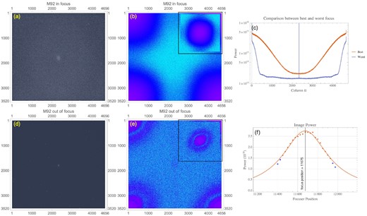
The images of M92 (globular cluster in Hercules) by our refractor II. In (f), we can see from the ‘Image power’ plot that our fit finds the focuser position in a dense star field.
The average of the focus positions found by the four estimators shown in Table 1 is (11676 ± 1) for the Fm data, and (11692 ± 1) for the HFDm data. In this example, all four estimators found results that are within CFZ for both the Fm and HFDm data. And they have the same spread as well.
5.3 Schmidt–Cassegrain telescope
The SCT that we used in the following test is a Celestron EdgeHD 800 which has an aperture of 8 arcsec and focal ratio F/10. It is equipped with a DC motor focuser from JMI. Since the JMI focuser does not use a stepper motor, the steps reported here are emulated values. We do not have the calibration that tells us the travel distance of the focuser per step because of the way the JMI focuser is connected to the SCT focusing mechanism, and the idiosyncrasies of the SCT focusing mechanism itself. The imaging CMOS camera is a ZWO ASI1600MM-P cooled camera (3.8 × 3.8 |$\mu {\rm m}^2$| square pixel).
The CFZ for this setup is 249 |$\mu$|m for green light (510 nm). Unfortunately, since we do not have the focuser calibration, the best we can do is to make an educated guess of the CFZ in terms of emulated step size. We do this by noticing that any measurable change in the HFD requires between 50 and 80 steps. Therefore, we will use this range as the estimate of the CFZ.
5.3.1 SCT pointed at a galaxy (M63)
We pointed our SCT at the Sunflower Galaxy (M63) for this test. A feature of an SCT is that when it is de-focused, the star images look like doughnuts because of the obstruction from the secondary mirror. As expected, we can see from Fig. 5(d) that the image of each star resembles a doughnut when de-focused. The doughnut effect adds more bumps to the spectrum in Fourier space, which we can see in Fig. 5(c). We want to see whether Fm is affected by this effect.
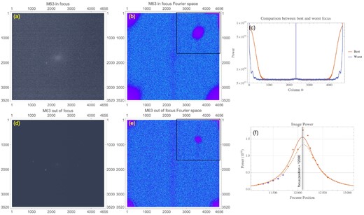
We pointed our SCT (Celestron EdgeHD 800) with a ZWO CMOS camera (ASI1600MM-P) at M63 (Sunflower Galaxy). The images shown here are after 7 s exposure. The (a) in-focus and (d) out-of-focus images in real space are both lightly stretched. After applying a 2D FFT to the real images, we see that there are clear bumps in the blue line of (c). These bumps come from the doughnuts. In (f), the ‘Image power’ plot contains two fits: a fit that ignores five outliers (continuous red line), and a fit that has no outliers (red dashed line).
Unfortunately, the quality of the data is not as good when compared to the refractor data. This is due to the entire focusing train of the SCT not having proper linear motion that is reliably reproducible. But despite these shortcomings, we can see from Fig. 5(f) that the Fm data can be fitted to all the data points or with five outliers in the tail, i.e. power from images that contain doughnuts, removed. (Note: This is done in our program by specifying at most 8 or 0 outliers for the S-estimation algorithm.) The focus position when all the data points are used is 12 115 emulated focus steps. While with five outliers ignored, we find the focus position to be at 12 090 emulated focal steps. The difference between the two results is 25 emulated focus steps that is within our estimate of the CFZ for this telescope/camera combination. This result means that Fm is not affected by doughnuts in the tails.
For comparison, when we use the HFDm data, the fit finds the focus position to be at 12 091. Thus, both Fm and HFDm data have yielded essentially the same focus position that is within our estimated CFZ.
The average of the focus positions found by the same estimators shown in Table 1 is (12106 ± 9) for the Fm data, and (12091 ± 0) for the HFDm data. In this example, all four estimators found results that are within the estimated CFZ, and for the HFDm data, they found the same focus position with zero spread.
5.4 2 m Ritchey–Chrétien–Coudé telescope
After our successful Fm tests with small telescopes, we had the opportunity to test Fm on the 2 m RCC at the Rozhen NAO. R. Bogdanovski (Rozhen NAO) and M. Minev (Rozhen NAO) collected images for us. The RCC has a focal ratio F/8 and is equipped with a focuser that has an absolute encoder. The absolute encoder has a resolution of 10 |$\mu$|m. The focuser has no backlash because of the absolute encoder. The CCD camera used for these images has a pixel size of (13.5 × 13.5) |$\mu {\rm m}^2$| square pixel. The CFZ for this setup is 159 |$\mu$|m for green light (510 nm).
5.4.1 RCC pointed at a nebula (IC1396)
The RCC was pointed at the Elephant Trunk Nebula (IC1396) for this test. Like the SCT, when it is de-focused, the star images look like doughnuts because of the obstruction from the secondary mirror. The collimation of the RCC was not perfect when the data were taken and so the stars are not point like even when in focus (see Fig. 6a). There is also a lot of structure in the Fourier space data shown in Figs 6(b) and (e). It is interesting that Fig. 6(c) shows that these structures are smoothed out because of the first integral in Fm. However, the doughnut structure of the stars is preserved because these curves clearly show bumps. But these bumps do not affect the ‘Image Power’ from our plot shown in Fig. 6(f). The fit to the data with Fm finds the focus position to be 81.13 mm. When we apply HFDm to the same images, the focus position is 81.11 mm. These two results show that both Fm and HFDm agree because they are within the CFZ.
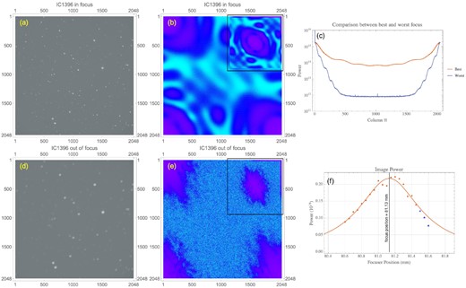
The 2 m RCC was pointed at IC1396 (Elephant Trunk Nebula). The images shown here are after 5 s exposure. The (a) in-focus and (d) out-of-focus images in real space are not stretched here. After applying a 2D FFT to the real images, we see that the results are quite different from the those taken by small telescopes. In (f), the ‘Image power’ fit has three outliers.
The average of the focus positions found by the four estimators shown in Table 1 is (81.130 ± 0.000) mm for the Fm data, i.e. all four estimators found the same results for Fm. Using HFDm, the four estimators found the focus position to be (81.111 ± 0.004) mm. In this instance, both Fm and HFDm agree because both are within the CFZ.
6 EFFECTS OF SATURATION
Fm does not work well when there are saturated stars in the image. We show an example of the effect of a saturated star by pointing a Takahashi FSQ106 refractor at Deneb (1.25 mag). The FSQ106, has an aperture of 106 mm and focal ratio F/5. It is equipped with a MoonLite focuser (0.269 |$\mu$|m/step) that has zero backlash. The imaging colour CCD camera is a SBIG STF8300C (5.4 × 5.4 |$\mu {\rm m}^2$| square pixel).
The effect on Fm as the exposure time is increased is shown in Fig. 7. For a short exposure time of 100 ms, Fm behaves as expected. But as the exposure time is increased to 250 ms, a dip appears. This is because the image of Deneb is saturated near focus. Finally, when Deneb is overexposed at 4 s, the expected Lorentzian peak completely vanishes and is replaced by a valley.
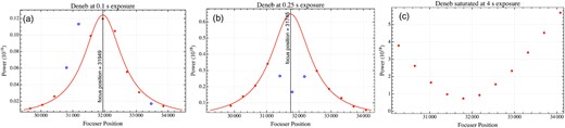
These plots show the effect of performing Fm with Deneb in the imaging frame. (a) For a short exposure of 100 ms, Fm finds the focusing position. (b) When the exposure time is increased to 250 ms, Deneb becomes saturated near focus that creates a dip in the Lorentzian. (c) Finally, when the exposure time is 4 s, the expected maximum at focus becomes a minimum.
The reason can be seen in Fig. 1 where we have drawn a dashed line to represent the saturation threshold. Let us suppose that the star image is truncated above this threshold, i.e. saturation. Then, it is immediately obvious that its power contribution is reduced because its peak is truncated. The power is further reduced as the star becomes more in focus because the base of the star image shrinks and most of the power contribution is above the threshold level.
Therefore, during focusing, we have to be careful not to have any saturated stars in the image or to apply an algorithm to damp down its effect.
One way to do this is to reduce the exposure time. But reducing the exposure to very short values has some drawbacks. It reduces the contributions of the other stars to the power function |$\bar{\cal P}_{\rm image}$|. Also, shorter exposures make the process more prone to seeing fluctuations. Therefore, we are currently testing software based methods that prevent the creation of the valley shown in Fig. 7(c) when saturated stars are in the image.
One solution is to define a new maximum that is smaller, e.g. |$\rm {max}_{\rm new}=\varphi \cdot \rm max+\rm min$|, where |$\rm max$| is the largest value supported by the image format and |$\rm min$| is the lowest value of any pixel in the given image. The variable φ is some numerical constant that has been shown to deliver good results for the bit depth of the used image format.
We first check whether pixels with a value of |$\rm max$| are in the image. If that is the case, we search for all pixels whose value is |$\ge \rm {max}_{\rm new}$| and replace them by |$\rm {max}_{\rm new}/2$|, which is the average of |$\varphi \cdot \rm max$| and |$\rm min$|. For the 16 bit images where we tested this procedure, we found that a value of φ = 0.01 delivered good results. The method gives both a smooth outer region of the saturated star and a flattened profile that is no longer saturated. For our example with the saturated star Deneb, this method yields a power curve whose fit has the same focus position that would be computed from parts of the image without the saturated star.
7 FOCUSING SIMULATION
One way to compare HFDm and Fm is to simulate multiple focusing runs by selecting a smaller subset of images from a much larger image data set. We can do the following:
We take a large series of images that are spaced less than the CFZ. We chose the starting and ending focuser positions so that they bracket the focus position. Furthermore, these images are taken as quickly as possible so that the ambient temperature does not change during this process.
We define the best focus position to be the image that has the largest number of identifiable stars.
We choose a fixed focuser increment that will allow us to select a much smaller subset of images. These selected images are spaced consecutively at the focuser increment.
We fit these images to both HFDm and Fm to see how well they match to the best focus position.
The telescope that we will use for this experiment is the same Takahashi FSQ106 that was described in Section 6. In these measurements, the images have not been de-Bayered and each image is the result of 4 s of exposure. The CFZ for this setup is 62 |$\mu$|m for green light (510 nm). The CFZ in terms of focuser step size is 230.

We used a plate solving program, astap, to determine the number of stars in each image. The image with the largest number of stars is when the focuser is at zmax stars = 31 972. We will define zmax stars as the best focuser position. When we do this, we can see that the difference between Fm and the best focuser position is 46 steps and HFDm and the best focuser position is 88 steps. So, even although both Fm and HFDm found focus positions that are within the CFZ of zmax stars position, we can see that Fm is closer.
7.1 Simulation
Now, we can simulate a typical focusing run by selecting 5–8 images per run. We constrain the selection of the images of each run by making sure that each selection contains at least one image from the first 10 images and the last image is within the last 10 images. We constrained the selections this way so that each run brackets the best focus position and not skewed to one side.
Fig. 9 shows the results of our simulation. We can see that the mean of the Fm focus positions is always closer to zmax stars than the HFDm focus positions. But, we have to note that the difference between both methods and w.r.t. zmax stars is within the CFZ, so in principle, both methods agree where the best focus position is. Finally, it is also interesting, that both methods have found focus positions that are always larger than zmax stars.
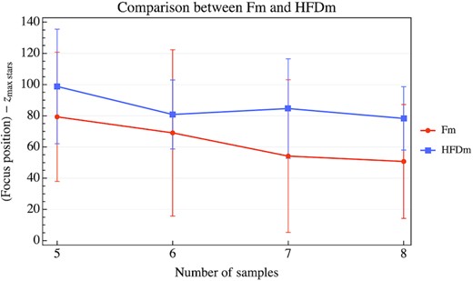
This figure shows the results of a simulated focusing run that samples 5–8 images from a population of 50 images. It is clear that the mean of the Fm focus positions is always closer than HFDm to the maximum star focus position. But the difference between both methods and w.r.t. zmax stars are within the CFZ.
From this simulation, we can say that for best results, we should have at least seven samples for either methods. But five samples is still adequate for finding the best focus position.
8 STRENGTHS OF Fm
Fm does not suffer from the problems HFDm that are listed below. Our studies in Section 5 show that when the estimators shown in Table 1 are applied to the data points generated by Fm, the results always have a spread less than the CFZ. But when the same estimators are applied to the data points generated by HFDm the spread can be larger than the CFZ. Our simulated focusing runs in Section 7 also show that both Fm and HFDm are comparable in performance, with perhaps a slight edge to Fm. However, as we have discussed in Section 6, we have to be careful about not saturating any of the stars during focusing.
We summarize here the weaknesses of HFDm:
Required detection of stars Star detection is absolutely required in HFDm because the HFD of each detected star has to be calculated. Unfortunately, due to CCD/CMOS read noise, sky glow noise, noise from light pollution, and hot pixels, the star detection algorithm has to be hand tuned to only detect stars and not other structures that look like stars. In contrast, Fm does not use star detection.
Noisy HFD measurements The problems with HFD measurements are the following:
As focus gets close, the HFD actually becomes noisier as its value becomes smaller. This is because when the star width is narrower, its fractional error becomes larger.
Far away from focus, the out-of-focus stars can be too dim to get a good HFD measurement or even be detected as stars. From our experience, even if HFDm detects these stars, the values of HFD in the tails are nearly always wrong.
These problems manifest themselves when we apply our robust estimators to the same data and they yield a much wider swath of focus positions than Fm. We have already seen this in Section 5.1.1.
HFDm step size The focuser step size between each image has to be tuned for every telescope/camera combination in HFDm. It cannot be too small or else there will not be a sufficient change in the HFD between each position. If it is too large, star detection may fail because each star becomes too de-focused. Consequently HFDm will fail because star detection has failed. In comparison, the Fm step size can be chosen to be half the CFZ for each telescope/camera combination.
Due to the superior results of Fm for obtaining the focus point estimation, we have written a small console application called fm. It expects the path to a folder with a small number of images in fit format versus focuser position. The power of each image is calculated for each focuser position that is then used to compute the best focus position with a user selected estimator algorithm. The user also selects the parameters used by the estimators. We have limited the maximum number of images required by fm to less than 24 images to keep the algorithm fast under all circumstances. We have found that fm needs about eight images for a good precise fit, but usually less than 17 images is sufficient. The source code of our application was published under MIT license at Schulz (2021). It comes with extensive documentation and can be compiled on Windows, Mac OS X, and Linux.
9 CONCLUSION
We have demonstrated that Fm works well for finding the focus position for both small and large telescopes. In the context of automation, it is automatic because it does not require tuning of any parameters except for the setting of the exposure time. This is in contrast to HFDm that not only requires setting of the exposure time, it also requires proper tuning of both star detection and focuser step sizes. In our experiments, we have found that, unlike HFDm, Fm shows a strong degree of independence from the choice of estimator. This means that the user can be confident that the focus position found by Fm is independent of the choice of the estimator. We have published a library that exports the algorithms and methods described in our paper as a c++application program interface (API), see Schulz (2021). The API was kept as simple as possible so that bindings to other languages, for example, python, can be easily generated with semi-automated tools. Finally, we provide a small console application for Windows, Mac OS X, and Linux under MIT license that uses the library to compute the best focus position of a telescope. In conclusion, with Fm, we have increased by one the number of automatic focusing methods available for professional and amateur telescopes alike.
ACKNOWLEDGEMENTS
We wish to thank the following people:
(i) Ivaylo Stoynov, author of the Astro Photography Tool (apt) application, who kindly allowed us to discuss our thoughts about AutoFocusing on the forum pages that he hosts. He also introduced us to Dr. R. Bogdanovski.
(ii) Dr. Rumen Bogdanovski (Institute of Astronomy and National Astronomical Observatory (NAO), Bulgarian Academy of Sciences) and co-author of indigo who arranged for some telescope time with the 2 m RCC for the collection of data shown in Fig. 6.
(iii) Milen Minev (Institute of Astronomy and NAO, Bulgarian Academy of Sciences) who collected the data shown in Fig. 6.
(iv) Dr. James Annis (Fermilab Cosmic Physics Center) who read our paper and encouraged us to publish these ideas.
(v) Dr. Adam Popowicz (Silesian University of Technology, Institute of Automatic Control) for his suggestion of a focusing simulation that we discussed in Section 7.
DATA AVAILABILITY
The data used in this paper are available upon request from the authors.
Footnotes
The full width half-max method (FWHMm) is used by sharpcap. FWHMm is the predecessor to HFDm.
To the authors’ knowledge, there is only one program, called sharplock, that does not use HFD. It uses the astigmatism of a star image for determining focus. See Baudat (2014).
This is the largest telescope in south-east Europe.
The idea of replacing statistical variables by their means to glean insight into the behaviour of the bulk is not new. This is the idea behind mean field theory. Whether it is plausible here is demonstrated by the good behaviour and fits to empirical data.
For example, in HFDm, the model that connects the HFD to focuser position is a hyperbola which has the form x2/a2 − y2/b2 = 1. We use the hyperbola to fit to the HFD data in Section 7.
We have added an inset to all the Fourier plots which has zero frequency at the centre. This is for readers who are more comfortable with this type of representation. We do not process the Fourier data in this shifted zero format.
