


ABSTRACT
The density of dark matter near the Sun, ρDM, ⊙, is important for experiments hunting for dark matter particles in the laboratory, and for constraining the local shape of the Milky Way’s dark matter halo. Estimates to date have typically assumed that the Milky Way’s stellar disc is axisymmetric and in a steady-state. Yet the Milky Way disc is neither, exhibiting prominent spiral arms and a bar, and vertical and radial oscillations. We assess the impact of these assumptions on determinations of ρDM, ⊙ by applying a free-form, steady-state, Jeans method to two different N-body simulations of Milky Way-like galaxies. In one, the galaxy has experienced an ancient major merger, similar to the hypothesized Gaia–Sausage–Enceladus; in the other, the galaxy is perturbed more recently by the repeated passage and slow merger of a Sagittarius-like dwarf galaxy. We assess the impact of each of the terms in the Jeans–Poisson equations on our ability to correctly extract ρDM, ⊙ from the simulated data. We find that common approximations employed in the literature – axisymmetry and a locally flat rotation curve – can lead to significant systematic errors of up to a factor ∼1.5 in the recovered surface mass density ∼2 kpc above the disc plane, implying a fractional error on ρDM, ⊙ of the order of unity. However, once we add in the tilt term and the rotation curve term in our models, we obtain an unbiased estimate of ρDM, ⊙, consistent with the true value within our 95 per cent confidence intervals for realistic 20 per cent uncertainties on the baryonic surface density of the disc. Other terms – the axial tilt, 2nd Poisson and time-dependent terms – contribute less than 10 per cent to ρDM, ⊙ (given current data) and can be safely neglected for now. In the future, as more data become available, these terms will need to be included in the analysis.
1 INTRODUCTION
The local dark matter density, ρDM, ⊙, is an estimate of the density of dark matter (DM) near the Sun, typically averaged over a small volume of width ∼0.2–1 kpc and height ∼0.2–3 kpc (e.g. Read 2014). In combination with other Galactic information, including the rotation curve, it yields an estimate of local shape of the Milky Way’s dark matter halo that can be used to test alternative gravity models and galaxy formation theories (e.g. Read 2014). It is also an important input in the quest to discover particle dark matter (e.g. Bertone, Hooper & Silk 2004; Roszkowski, Sessolo & Trojanowski 2018). The expected signal strength in many experimental searches, such as direct detection experiments searching for elastic scattering events, directly depends on the value of ρDM, ⊙. An accurate estimate is, therefore, needed to measure particle properties in the event of a detection.
Recent estimates of ρDM, ⊙ make use of a variety of methods (e.g. de Salas & Widmark 2021). ‘Local’ methods use Jeans and/or distribution function models over small volumes near the Sun (e.g. Xia et al. 2016; Sivertsson et al. 2018; Guo et al. 2020; Salomon et al. 2020). ‘Global’ methods use stellar tracers over larger volumes (e.g. Cole & Binney 2017; Wegg, Gerhard & Bieth 2019), or use the Milky Way’s circular velocity, assuming that its dark matter halo is spherically symmetric (e.g. Benito, Cuoco & Iocco 2019; de Salas et al. 2019; Karukes et al. 2019). More recently, newer methods have been introduced, like ‘made to measure’ (e.g. Syer & Tremaine 1996; Bovy, Kawata & Hunt 2018), and a recent attempt to harness the Milky Way disc’s disequilibrium to estimate ρDM, ⊙ (Widmark et al. 2021). Some studies exploit the vertical kinematics of stars up to a height |$z \sim 1\!-\!3\, \mathrm{kpc}$| above the Galactic disc (e.g. Xia et al. 2016; Sivertsson et al. 2018; Guo et al. 2020; Salomon et al. 2020), while others use a similar methodology much closer to the plane (<200 pc; Schutz et al. 2018; Buch et al. 2019; Widmark 2019). The former has the advantage that dark matter makes up a larger fraction of the mass at these heights, but the disadvantage that it is less local. Recently, Cole & Binney (2017) have fit a global distribution function model to a wide range of data for the Milky Way, while Wegg et al. (2019) fit the azimuthally averaged Jeans equations to a sample of |$\sim 16\, 000$| RR Lyrae stars from Gaia DR2 over a Galactocentric distance range of 1.5 < R < 20 kpc. A review of historic estimates of ρDM, ⊙ is given in Read (2014), and more recent estimates are reviewed in de Salas & Widmark (2021); we summarize recent local estimates in Fig. 1.1
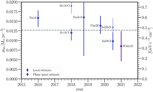
Recent local estimates of the local dark matter density, ρDM, ⊙. The mean of all data points is shown by the horizontal dashed line. At first sight, the agreement seems to be excellent as most data points agree within in their 68 per cent confidence intervals (error bars, as marked). However, there remain potentially significant sources of systematic error. The light blue points show alternative, disfavoured, measurements of ρDM, ⊙ using different tracer stars. In the case of Sivertsson et al. (2018), these are ‘α-old’ stars that are kinematically hotter; for Salomon et al. (2020), these are stars in the Northern hemisphere that show more prominent signs of disequilibrium than those in the Southern hemisphere. Finally, the purple data point shows a recent determination from Widmark et al. (2021) that is distinct from the other local methods in that it harnesses the fact that the Milky Way disc is wobbling and ringing. (Data taken from Xia et al. 2016; Sivertsson et al. 2018; Buch, Leung & Fan 2019; Guo et al. 2020; Salomon et al. 2020; Widmark et al. 2021).
Most of the above estimates of ρDM, ⊙ assume a steady state pseudo-equilibrium such that the distribution function of the tracers stars has no explicit time dependence; most additionally assume axisymmetry. We have known for a long time that the Milky Way is not axisymmetric, displaying prominent spiral arms and a bar (e.g. Hou & Han 2014; Camargo, Bonatto & Bica 2015; Hilmi et al. 2020). Furthermore, with the advent of large surveys like the RAdial Velocity Experiment and the Sloan Digital Sky Survey, we have discovered that the Milky Way disc is ‘wobbling’, with significant vertical and radial oscillations in density and velocity (Widrow et al. 2012; Williams et al. 2013). The ESA–Gaia satellite has brought this into sharp focus (Schönrich & Dehnen 2018; Bennett & Bovy 2019). A major discovery that has come from its second data release (DR2) is the detection of ‘phase-space spiral’ in the local stellar disc (Antoja et al. 2018). Several authors have provided potential explanations for this feature (see e.g. Antoja et al. 2018; Binney & Schönrich 2018; Laporte et al. 2018b; Bland-Hawthorn et al. 2019; Khoperskov et al. 2019; Laporte et al. 2019). When dissecting the phase-space spiral in stellar ages, Laporte et al. (2019) detect it at all stellar ages down to very young ages |$\sim 0.5\!-\!1\, \rm {Gyr}$| pointing towards a recent perturbation (as opposed to bar buckling). Taken at face value, this is consistent with orbital time-scales of Sagittarius (Johnston, Law & Majewski 2005; Peñarrubia et al. 2010) and those derived for phase-mixing time-scales through toy-modelling in the original study of Antoja et al. (2018), favouring the impact scenario (Laporte et al. 2018b). This is currently the only mechanism able to simultaneously reconcile perturbations on large and small scales in the disc (Slater et al. 2014; Price-Whelan et al. 2015; Bergemann et al. 2018; de Boer, Belokurov & Koposov 2018; Schönrich & Dehnen 2018; Laporte et al. 2020a). Although the details of the perturbation remain to be worked out, most authors agree that some form of disequilibrium (i.e. a non-steady-state disc) is at work in the solar neighbourhood and across the Galaxy both vertically and radially (Minchev et al. 2009; Gómez et al. 2013; Monari, Famaey & Siebert 2016; Antoja et al. 2018; Hunt et al. 2018; Laporte et al. 2018b; López-Corredoira et al. 2020; Xu et al. 2020).
Given that the Milky Way disc is not axisymmetric nor in a steady state, we can reasonably ask how secure recent estimates of ρDM, ⊙ are. Early work demonstrated that Jeans methods, that assume an axisymmetric potential and separable radial and vertical stellar motions, are able to obtain a statistically unbiased estimate of ρDM, ⊙ when applied to a few thousand tracer stars, even in the face of prominent spiral arms and a bar (Garbari, Read & Lake 2011). However, the Gaia data presents us with millions of tracer stars that extend much higher above the disc (e.g. Read 2014). For this quality and extent of data, systematic errors will almost certainly dominate the error budget, especially if the Milky Way’s disc lies much further from a pseudo-equilibrium state than was assumed in Garbari et al. (2011). More recently, Haines et al. (2019) have applied an axisymmetric Jeans method to mock data from an N-body simulation of the Milky Way that includes a recent encounter with a Sagittarius-like dwarf galaxy (Laporte et al. 2018b). They find that, in this case, estimates of ρDM, ⊙ can become systematically biased by up to a factor of ∼1.5, which is substantially larger than the formal uncertainties on ρDM, ⊙. Indeed, this could explain systematic variances in ρDM, ⊙ reported in the literature for estimates derived from different stellar tracer populations in the disc, and between red clump stars in the Northern and Southern hemispheres (see Sivertsson et al. 2018; Salomon et al. 2020 and Fig. 1).
To address the above issues, in this paper we assess how well a steady-state free-form (non-parametric)2 Jeans method can recover ρDM, ⊙ from a non-axisymmetric, non-steady state disc. We further develop the mass modelling method introduced in Silverwood et al. (2016) and Sivertsson et al. (2018) to generalize the functional form of the tracer density and velocity anisotropy profiles, and to remove any assumption of axisymmetry. We then apply this method to mock data generated from a simulated ‘wobbling’ disc, seeded by either an ancient massive merger or a more recent Sagittarius-like merger (this latter simulation is identical to the one used in Haines et al. 2019). We assume a ‘best-case’ scenario of zero observational uncertainties, a volume complete sample of tracer stars, and perfect measurement of all steady-state terms in the Jeans equation. This allows us to isolate the impact of common modelling assumptions on our recovery of ρDM, ⊙, carefully separating out bias induced by disequilibrium from bias due to other common assumptions, like axisymmetry. More realistic mocks should include the impact of observational uncertainties, survey selection effects, and the current impact of the Large Magellanic Cloud that is believed to be on its first infall and about a fifth of the mass of the Milky Way (e.g. Weinberg 1998; Besla et al. 2007; Gómez et al. 2015; Peñarrubia et al. 2016; Laporte et al. 2018a,b; Erkal et al. 2019; Garavito-Camargo et al. 2019; Read & Erkal 2019; Besla et al. 2019; Donaldson, Petersen & Peñarrubia 2021). We will consider these additional complications in future work.
This paper is organized as follows. In Section 3, we describe our mass modelling method that builds on the free-form method presented in Silverwood et al. (2016) and Sivertsson et al. (2018). In Section 2, we describe the N-body simulations that we use in this work, and how we generate our mock data from these simulations. In Section 4, we present the results from applying our method to the mocks. In Section 5, we discuss our results and their broader implications for estimating ρDM, ⊙. Finally, in Section 6, we present our conclusions.
2 SIMULATIONS
2.1 Description of the simulations
We test our free-form Jeans method (Section 3) on two N-body simulations of MW-like galaxies, both of which are perturbed by an external, smaller, galaxy. One of the simulations – GSE60 – is an N-body simulation of a MW-like galaxy that experienced an M ∼ 1011 M⊙ merger ∼4 Gyr ago, and then evolved without any further external perturbations (Garbari 2012). In this simulation, the MW-like galaxy is identical to that used in Garbari et al. (2011), which is set up as described in Widrow & Dubinski (2005) (see Table 1 for a summary of its properties). The motivation for this case stems from the recent analysis of the local stellar halo which shows that more than half of the |$\rm {[Fe/H]\lt -1\, dex}$| stars appear to originate from a single massive accreted system – the ‘Gaia–Sausage–Enceladus’ (GSE) satellite galaxy (e.g. Belokurov et al. 2018; Haywood et al. 2018; Helmi et al. 2018; Mackereth et al. 2019) that had a mass of |$\sim 1.0\times 10^{11}\, \mathrm{M}_\odot$| (∼1/10 total mass ratio). We will refer to this simulation as GSE60, where ‘60” refers to the initial orbit inclination, in degrees, of the merger with respect to the main galaxy’s disc plane (Garbari 2012).
The N-body simulations used to generate mock data. From left to right, the columns give: the simulation label; number of particles, mass, and force softening of each component; the half mass scale length and height of the disc prior to the satellite merger; and some notes on each simulation (see Section 2 for details).
| N | M | ϵ | R1/2 | z1/2 | ||
|---|---|---|---|---|---|---|
| (106) | (|$10^{10}\, {\rm M}_\odot $|) | (kpc) | (kpc) | (kpc) | Notes | |
| GSE60 | ∼1011 M⊙ satellite merger 4 Gyr ago | |||||
| Disc | 30 | 5.30 | 0.015 | 4.99 | 0.17 | – |
| Bulge | 0.5 | 0.83 | 0.012 | – | – | – |
| Halo | 15 | 45.40 | 0.045 | – | – | – |
| Sgr6 | 0.8 × 10¹¹ M⊙ merger, ongoing | |||||
| Disc | 5 | 6.0 | 0.03 | 5.88 | 0.37 | – |
| Bulge | 1 | 1.0 | 0.03 | – | – | – |
| Halo | 40 | 100 | 0.06 | – | – | – |
Our main emphasis, however, will be on the second N-body simulation – Sgr6 – described in Laporte et al. (2018b), set up using GALIC (Yurin & Springel 2014). In this simulation, a Sagittarius-like dwarf galaxy (|$M_{200} \sim 0.6\times 10^{11}\, \mathrm{M}_\odot$|) is accreted on to a previously unperturbed Milky Way-like galaxy (see Table 1 for a summary of its properties). Following the Gaia DR2 release, Laporte et al. (2019) re-analysed this N-body simulation, finding that the repeated impacts of the orbiting Sagittarius-like dwarf galaxy excites oscillations in the disc that reproduced many of the newly uncovered features in the Gaia DR2 data (Gaia Collaboration 2018). We will refer to this simulation as Sgr6, where ‘6’ refers to the snapshot location in time, t = 6 Gyr from the start of the simulation, which is the same snapshot as used in Haines et al. (2019). This time was not chosen with intention to use a ‘present-day’ snapshot for the MW-Sgr-like system, but rather specifically pick a time shortly following a pericentric passage by a satellite. Note that we also applied our Jeans analyses method to earlier snapshots in the simulation, for which the MW-like galaxy had not yet been perturbed. Our method worked very well on this unperturbed disc and so, for brevity, we do not discuss those results here.
The two simulations investigated are complementary. The GSE60 simulation shows a MW-like galaxy that has undergone an ancient but violent merger from which the system has since had time to relax. The Sgr6 simulation, on the other hand, considers the impact of an ongoing perturbation of the MW-like galaxy. A visual impression of the Sgr6 simulation at t = 6 Gyr is shown in Fig. 2, where the top and bottom panels show a face-on and edge-on view of the stellar disc, respectively. In this snapshot, the remnant of the Sagittarius-like dwarf (purple cross and dots) is moving downwards, towards the MW-like disc. For a visual impression of the GSE60 simulation (that has no ongoing merger), see Garbari et al. (2011).
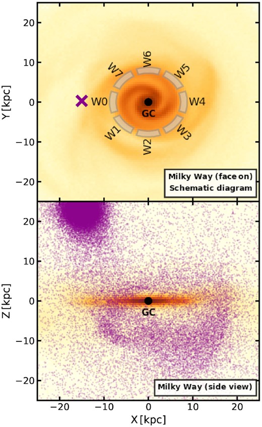
Face-on (top) and edge-on (bottom) view of the Sgr6 simulation at t = 6 Gyr from Laporte et al. (2018b), showing the ongoing merger of a Sagittarius-like dwarf (purple cross and dots) with an MW-like host galaxy (yellow-orange). The top panel shows the location and extent of the eight wedges in the disc plane from which we extract our mock data.
2.2 Generating the mock data
When analysing the N-body simulations, we divide the galactic disc into eight ‘wedges’, with a small gap between each wedge, as shown in Fig. 2. We analyse each wedge separately, essentially imagining eight different locations in the simulated galaxy where the Sun might be placed. Each wedge spans a radial range 7.5 < R < 8.5 kpc from the galactic centre, subtends an angle of |$\pi/5$|, and is centred around |$\frac{\pi }{4}N-\pi$|, where N ∈ [0, 7] is the number of the wedge, as shown in Fig. 2. The wedges used are identical for both the GSE60 and Sgr6 simulations.
When generating the mock data from each wedge, the data are binned using equidistant bins in height, z. We assume ‘ideal data’ with zero measurement uncertainty, volume complete tracer stars, and consistent photometric and kinematic tracer populations (see e.g. the discussion on this in Read 2014). This will allow us to focus on how common modelling assumptions drive systematic errors on ρDM, ⊙. Furthermore, the tracer stars only include stars which originated in the Milky Way-like galaxy. This assumes that these can be observationally separated from the accreted stars using, for example, their distinct chemistry (e.g. Ruchti et al. 2015). We leave an exploration of more realistic uncertainties, selection functions, and inconsistency to future work.
The wedges in GSE60 and Sgr6 have 20 000–48 000 and 100 000–170 000 stars within ±2 kpc of z = 0, respectively. For Gaia, we can expect millions of tracers near the Sun (Read 2014), but after quality, magnitude, and colour cuts, and avoiding the high-extinction disc, this number is dramatically reduced. For example, Salomon et al. (2020) present a recent estimate of ρDM, ⊙ from Gaia DR2 red clump stars; after such cuts, their total sample is |$\sim 40\, 000$| stars, with half in the Northern and half in the Southern hemisphere. As such GSE60 and Sgr6 are indicative of the current Gaia sampling error.
3 THE MASS MODELLING METHOD
3.1 The Jeans–Poisson equations
Given an observed density of tracer stars, ν(R, ϕ, z) and their velocity moments |$\overline{v_{i}}$| and |$\overline{v_{ij}}$|, we can, at least in principle, solve equations (1) and (2) to determine the matter density, ρ(R, ϕ, z). Subtracting off the contribution from visible stars, gas and stellar remnants yields an estimate of the mean dark matter density in each wedge, ρDM, ⊙ (e.g. Read 2014).
We now discuss each of the terms in equations (1) and (2), common approximations in the literature that neglect some subset of these terms, and their likely importance for the determination of ρDM, ⊙.
3.2 The 1D approximation
Most work to date on estimating ρDM, ⊙ has employed something akin to the 1D approximation (e.g. Read 2014; Xia et al. 2016; Sivertsson et al. 2018; Guo et al. 2020; Salomon et al. 2020). Here, we will also use this approximation as our default method. However, we will then add in each of the missing terms from the Jeans equation one at a time to assess their importance. In all cases, we will assume a perfect measurement of each term as calculated directly from the simulations. This will allow us to determine which terms are important and which can be discarded and, in particular, whether we must include time-dependent terms in order to obtain a robust estimate of ρDM, ⊙. We now consider each of the terms neglected in the above 1D approximation in turn.
3.3 The rotation curve term
In Figs 3 and 4, we plot Δρ for each wedge in the GSE60 and Sgr6 simulations, respectively. We calculate Δρ directly from the known gravitational potential of the simulations, averaging over the size of the wedge weighted by the local tracer density. For the real Milky Way, we can estimate |Δρ| from the radial derivative of the local rotation curve as a function of height above the plane (e.g. Garbari et al. 2012; Li, Zhao & Yang 2019). We discuss this further in Section 5.
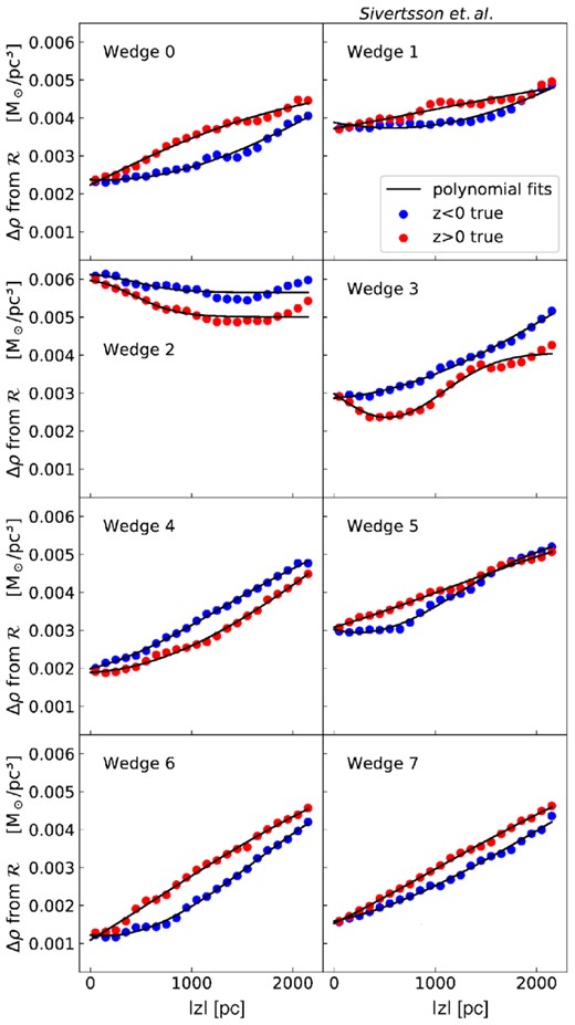
The rotation curve term contribution to the recovered local density for the GSE60 simulation as a function of |z| for the z > 0 (red) and z < 0 (blue) directions. The black lines are fits of the form shown in equation (7). Notice that in many of the wedges, |Δρ| approaches about half of the local dark matter density, |$\rho _{\mathrm{DM},\odot }\sim 0.01\, \mathrm{M}_\odot $| pc−2. As such, this is an important term that should not be neglected.
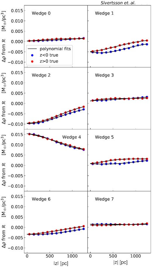
As Fig. 3 but for simulation Sgr6. Notice that for this simulation, in which the satellite interaction is still ongoing, in several wedges |Δρ| is now of the order of the local dark matter density, |$\rho _{\mathrm{DM},\odot }\sim 0.01\, \mathrm{M}_\odot\,$|pc−2. As with GSE60, this is an important term that should not be neglected.
As can be seen, across all wedges and both simulations |Δρ| can often be as large as ∼half of the local dark matter density. It is positive for all wedges in the GSE60 simulation, implying that one would underestimate the true underlying surface density if the |$\mathcal {R}$| term is neglected. By contrast, for the Sgr6 simulation, Δρ varies strongly between the wedges and can be positive or negative – an indication of significant non-axisymmetry. For wedge 4 in Sgr6, Δρ is comparable to ρDM, ⊙ and so neglecting it in the modelling will be a particularly poor approximation.
3.4 The 2nd Poisson term
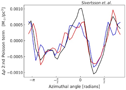
The 2nd Poisson term as a function of azimuthal angle, ϕ, averaged over the radial interval 7.5 < R < 8.5 kpc, for the Sgr6 simulation. The black line corresponds to z = 0, while the blue and red lines correspond to z = −1 kpc and z = 1 kpc, respectively. This term is everywhere less than 10 per cent of ρDM, ⊙ (also for the GSE60 simulation) and so can be safely neglected.
3.5 The tilt term
In Silverwood et al. (2016) and Sivertsson et al. (2018), we assumed a simple power law for the cross term of the velocity ellipsoid, |$\overline{v_R v_z} = A\left(\frac{z}{\rm kpc}\right)^n$|. As we shall show here, however, this is not sufficient to capture the behaviour of |$\overline{v_R v_z}$| in the simulations. For this reason, in this paper we generalize the treatment of |$\overline{v_R v_z}$|, measuring it, along with the radial scale length, h, directly from the simulation data for each wedge. To integrate over |$\mathcal {T}$| in equation (9), we fit a 3rd order polynomial in z to the simulation data, performing these fits separately for z > 0 and z < 0. This fit is performed jointly alongside the MultiNest fit to the other model parameters in our Jeans analysis (Section 4.3). As such, we show the tilt terms extracted from the simulations in this way later on the paper in Fig. 14.
3.6 The axial tilt term
In Fig. 6, we show |$\Delta \Sigma _\mathcal {A}$| for the Sgr6 simulation. This shows that the contribution of the axial tilt term is very small as compared to the true surface densities (Figs 7 and 8). (The results for the GSE60 simulation are similar and so we omit these for brevity.) We conclude that the contribution from the axial tilt term can safely be neglected.
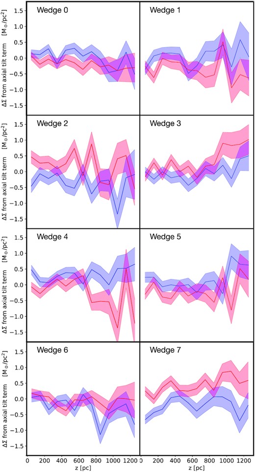
The size of the axial tilt term when interpreted as an effective surface density contribution, |$\Delta \Sigma _\mathcal {A}$| (equation 11) for the Sgr6 simulation. The data points for the z > 0 and z < 0 directions are shown with black dots and stars, respectively. Note that the red and blue bands, for the z > 0 and z < 0 directions, respectively, do not correspond to any analysis or fit; they are just to guide the eye. As compared to the total surface density (Fig. 8), |$\Delta \Sigma _\mathcal {A}$| is very small (of the order of 1 per cent of the total) and so the axial tilt term can be safely neglected in our analysis.
Recovered surface densities from Jeans mass modelling the GSE60 simulation. In this plot, we use the ‘1D approximation’ that neglects the tilt and rotation curve contributions to the Jeans–Poisson equations (equations 3 and Section 3.2). Each panel shows one of the eight wedges shown in Fig. 2. The blue and red bands show the 95 per cent credible regions for the recovered surface densities from the MultiNest runs in the z < 0 and z > 0 regions, respectively. The true values are shown as purple stars and dots, again for z < 0 and z > 0 regions, respectively (the stars and dots in this plot overlap to the point where they are indistinguishable).
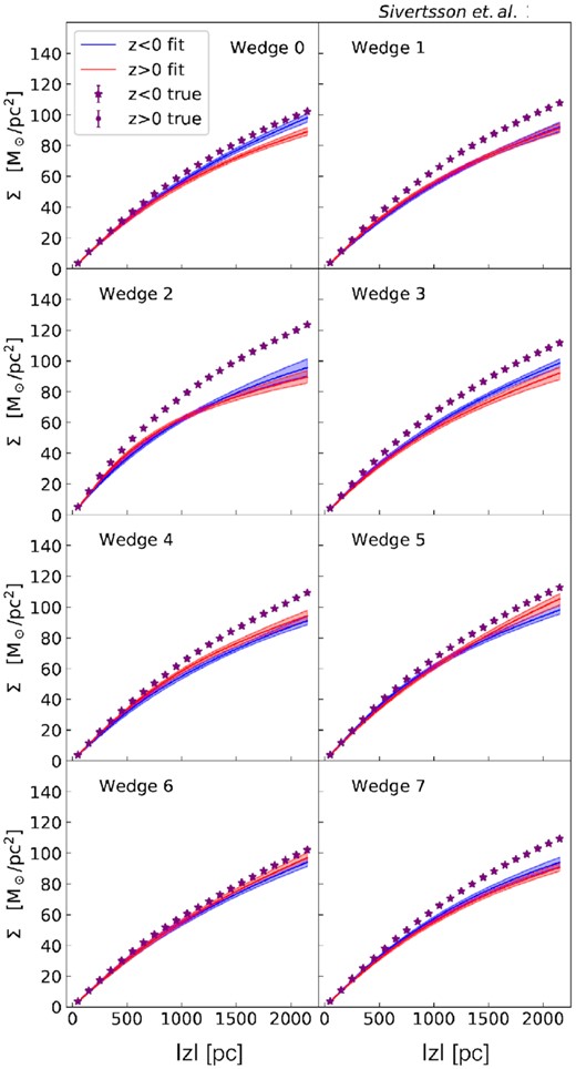
Recovered surface densities from Jeans mass modelling the Sgr6 simulation in the ‘1D approximation’. Lines and points are as in Fig. 7.
3.7 The explicit time-dependent term
The explicit time-dependent term in the Jeans equation (1) is challenging to measure from observations of a real galaxy, though it can be estimated by a careful elimination of all other terms, or through modelling inconsistencies between tracer populations with distinct vertical frequencies (Banik, Widrow & Dodelson 2017). In this paper, we take the former approach. By including all terms in the Jeans equations, any remaining bias in our recovery of ρDM, ⊙ must owe to the time-dependent term.
3.8 The tracer and mass density
Most studies in the literature to date assume an exponential form for the tracer density profile ν ∝ exp (− |z|/z0) which greatly simplifies the Jeans equations (e.g. Haines et al. 2019). However, we find that our perturbed N-body simulations can often depart significantly from this simple assumption. As such, we assume a much more general form for ν by fitting the ν data with several exponential segments, each over a smaller range in z. Each segment in the ν fit is given by an exponential function with its own scale height and normalization, adjusted so that the fit is continuous. The number of segments is adjusted so that a good fit to the tracer density is achievable while still maintaining a smooth function. This more general treatment of ν is possible thanks to our choice of solving the combination the Jeans–Poisson equations by integration rather than by differentiation (equation 4), making it straightforward for us to integrate the segment-wise fit to ν. It also has the advantage that the integrals in equations (4) and (5) are analytic. An example segment-wise fit to the tracer density data is shown in Fig. 12.
We divide the total matter density, ρ, into a contribution from baryons, ρb, and dark matter, ρDM, ⊙: ρ = ρb + ρDM, ⊙. We assume that ρDM, ⊙ is constant in each wedge,3 and we assume that ρb has the same shape as ν, with an uncertainty of 20 per cent on its normalization. Note that under these definitions, ρDM, ⊙ will include any contribution to the potential from stars and dark matter accreted from the satellite merger.
3.9 Model fitting, likelihood function and priors
We scan through the parameter space using the Bayesian nested sampling tool MultiNest (Buchner et al. 2014; Feroz et al. 2019) to find which model parameters provide the best fit to the observables |$\overline{v_z^2}$| and ν, as well as |$\mathcal {T}$|, when applicable.
We include |$\overline{v_z^2}$| data up to approximately two scale heights in ν and ρb, in line with Garbari et al. (2011). The scale heights vary significantly between the N-body simulations investigated here, in part because perturbations puff up the disc and hence increase the scale height. The individual limit of two scale heights maximizes the use of the data while avoiding the highest |z| bins that have very few stars and hence large statistical noise and bias. For ν, however, we include slightly larger values of |z| because the upper limit of the integral in equation (3) goes to infinity. Even though the contribution from higher |z| values is small because of the exponential fall-off of ν, the values of ν from the z regions just outside of the range used in |$v_z^2$| data can still have some impact on the evaluation of |$v_z^2$| from equation (3).
We set a linear prior on the dark matter density in the range |$10^{-3} \lt \rho _{\mathrm{DM},\odot }/ ({\rm M}_\odot \, {\rm pc}^{-3}) \lt 10^{-1}$|. We use a 20 per cent flat prior on the baryon density around the true value. For the tracer density priors, we make an initial fit to the data, setting 50 per cent flat priors on the best-fitting scale heights and a logarithmic prior on the normalization of ±2.5 dex around the true value. For the tilt, we make a polynomial fit to the data and then set a 50 per cent flat prior around the best-fitting values. For the rotation curve term, we fix the values to those extracted from the simulations – a best-case scenario.
4 RESULTS
In this section, we show the results from applying our Jeans method to the GSE60 and Sgr6 simulations, with and without the inclusion of the rotation curve and tilt terms in the steady-state Jeans–Poisson equations (1) and (2). (As discussed in Section 3, the 2nd Poisson term and the axial tilt term are small and so we neglect these.)
4.1 The 1D approximation
We begin by considering first the ‘1D approximation’ typically employed in the literature to date (Section 3.2). In Figs 7 and 8, we show the recovered surface densities4 for the GSE60 and Sgr6 simulations, respectively. As can be seen, for the GSE60 simulation, the results are generally rather poor. In all wedges, the surface densities are underestimated at more than 95 per cent confidence and in some cases by up to a factor of ∼1.5 (wedge 2). Only wedges 0 and 6 recover the true surface density within the 95 per cent confidence interval, and then only for z < 0 and z > 0, respectively. Worse, with the exception of wedge 0, the confidence intervals overlap for the z < 0 and z > 0 samples. Discrepancies between the dynamics of z < 0 and z > 0 stars has been invoked in the literature as a mark of disequilibrium dynamics (e.g. Haines et al. 2019; Salomon et al. 2020) and so the lack of such a signature could yield false confidence in the results.
The situation is similar for the Sgr6 simulation (Fig. 8). Only wedges 5 and 6 recover the surface density within the 95 per cent confidence band, while the worst wedge (4) is biased low by a factor of ∼1.4 for the z < 0 tracers.
4.2 Including the rotation curve term
In Figs 9 and 10, we show the recovery of the surface density when including the rotation curve term (equation 6 and Section 3.3). Notice that the recovery is now much improved for all wedges across both simulations, demonstrating the importance of including this term in the models. For GSE60, we now recover the input solution within the 95 per cent confidence bands for all wedges, except 2 and 3 for z > 0. Even in these cases, the PFds: Statistical bias is much smaller than previously, of the order of 5 per cent. There is a similarly good improvement for simulation Sgr6, though wedges 3, 6, and 7 all retain a bias larger than the 95 per cent intervals.


4.3 Including the tilt term
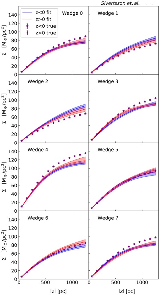
Fig. 11 shows our recovery of the surface density when including the rotation curve and tilt terms in our analysis (equation 9 and Section 3.5). This further improves our recovery of the input solution, demonstrating the importance also of this term. Now, combining the scatter in solutions from the z < 0 and z > 0 samples, there is no longer any bias larger than our 95 per cent confidence bands. There can still be bias, however, if only one of these samples is considered. For example, the z < 0 tracers in wedge 6 are systematically biased low. (We obtain already unbiased results for the GSE60 simulation without the tilt term (Fig. 9), and so omit an analysis of the GSE60 simulation including tilt, for brevity.)
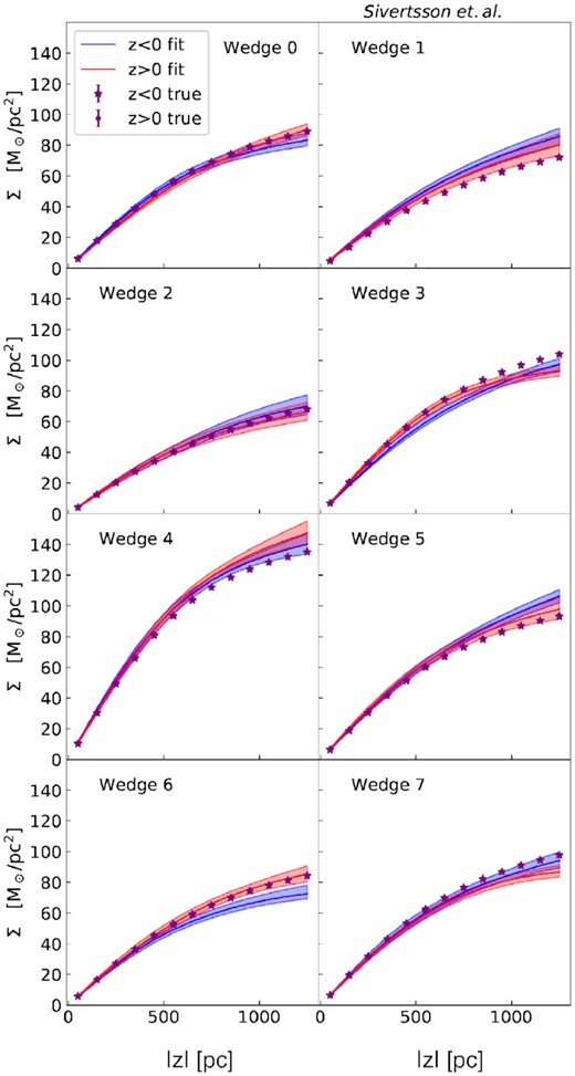
Recovered surface densities from Jeans mass modelling the Sgr6 simulation in the ‘1D approximation’, including the rotation curve and tilt terms. Lines and points are as in Fig. 7. Notice that the recovery is now further improved as compared to the analysis with just the rotation curve term (Fig. 10).
The quality of our fits to the tracer density ν(z), vertical velocity dispersion |$\overline{v_z^2}(r)$|, and tilt term for the Sgr6 simulation are demonstrated in Figs 12, 13, and 14, showing that this model gives an excellent recovery of the data for all wedges. In particular, notice that there is no obvious feature in the data that can predict which wedges will be most biased. Wedge 6 for the z < 0 tracers, for example, remains most biased after the inclusion of the rotation curve and tilt terms, but shows no particular feature in the data as compared to the other wedges.
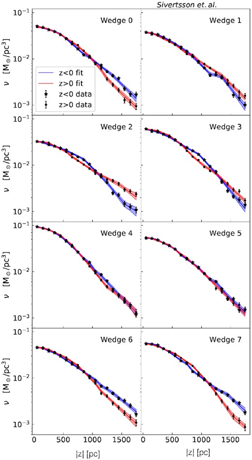
Example fit to the tracer densities from the same analysis of the Sgr6 simulation as shown in Fig. 11 (i.e. when including both the rotation curve and the tilt terms in the analysis). Conventions are as in Figs 8 and 13, but showing ν instead of Σ. Note that the fit to the ν data includes higher |z| values than the fit to the |$\overline{v_z^2}$| data, to increase the accuracy of our method (see Section 3.9 for details). The error bars on the data points include only Poisson noise and represent 1 standard deviation.
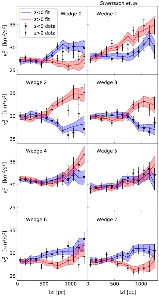
Example fit to the vertical velocity dispersions from the same analysis of the Sgr6 simulation as shown in Fig. 11 (i.e. when including both the rotation curve and tilt terms in the analysis). Conventions are as in Fig. 8 but showing |$\overline{v_z^2}$| instead of Σ. The error bars on the data points include only Poisson noise and represent 1 standard deviation.
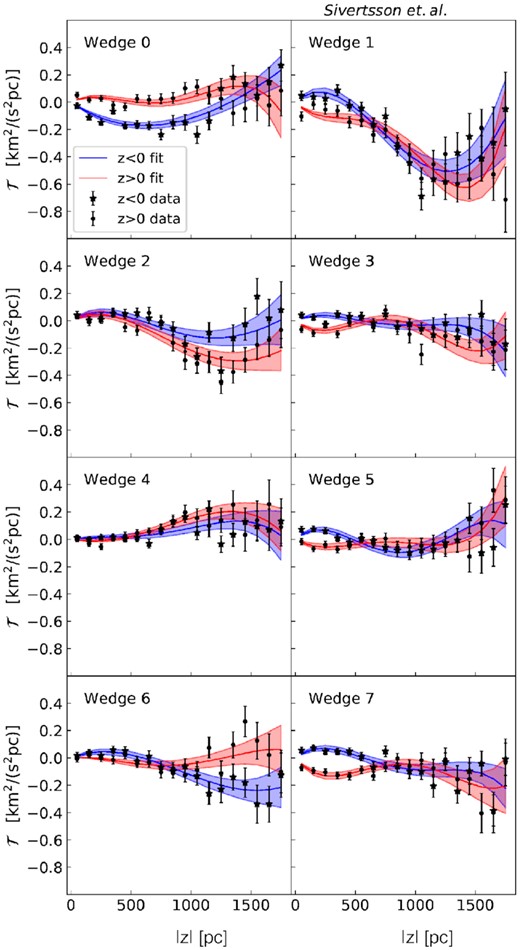
Example fit to the tilt term from the same analysis of the Sgr6 simulation as shown in Fig. 11 (i.e. when including the rotation curve and tilt terms). Conventions are as in Figs 8 and 13, but showing |$\mathcal {T}$| instead of Σ. The tilt terms are modelled as 3rd order polynomials. As for ν, we include higher |z| data points in the |$\mathcal {T}$| fit (see Section 3.9 for details). The error bars on the data points include only Poisson noise and represent 1 standard deviation.
4.4 Recovering the local dark matter density
In Figs 15, we show our recovery of ρDM, ⊙ for GSE60 (upper, including the rotation curve term), Sgr6 (middle, including the rotation curve and tilt terms) and Sgr6 (bottom, as the middle panel but using a tighter 1 per cent prior on the baryon density) simulations, shown as a function of wedge number.
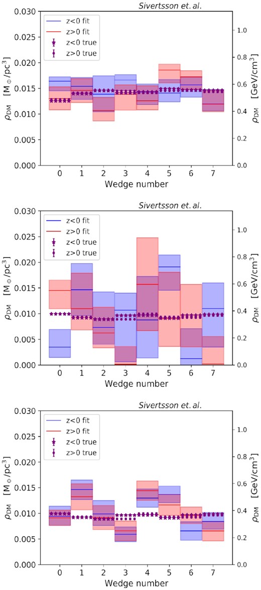
Recovery of the local dark matter density from Jeans mass modelling the GSE60 (upper, including the rotation curve term), Sgr6 (middle, including the rotation curve and tilt terms) and Sgr6 (bottom, as the middle panel but using a tighter 1 per cent prior on the baryon density) simulations, shown as a function of wedge number. The red and blue bands show the recovered values of ρDM, ⊙ with 2σ error bars for the z > 0 and z < 0 samples, respectively, while the purple dots and stars show the true values (from the simulations). The top two panels assume an error on baryonic surface density Σb of 20 per cent, comparable to current estimates; the bottom panel is relevant for the future once the baryon density is known to 1 per cent. Notice that the uncertainties are smaller for the GSE60 simulation due to the increased sampling in each wedge, while there is more bias in the Sgr6 simulation that becomes more visible once tighter priors are placed on the baryon density (bottom panel).
First, notice that with our default 20 per cent errors on Σb (top and middle panels), we recover ρDM, ⊙ within our quoted uncertainties for almost all wedges in both simulations, if we consider the combined uncertainty from the z > 0 and z < 0 analysis. Only wedge 0 for the Sgr6 simulation shows statistically significant bias, being too high above the disc and too low below the disc. In Fig. 16, we show the corresponding recovery of Σb for the Sgr6 simulation. In this plot, we see the same effect for wedge 0 but anticorrelated with the recovery of ρDM, ⊙. This indicates that we have correctly recovered the total surface density, but partitioned it incorrectly into dark matter and baryons for this wedge. This highlights the known degeneracy between Σb and ρDM, ⊙ (Sivertsson et al. 2018). We discuss this further in Section 5.
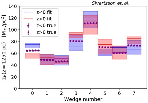
Recovery of the baryonic surface density at z = ±1250 pc (defined as |$2\int _{-1250}^0\rho \mathrm{d}z$| (blue bands) and |$2\int _0^{1250}\rho \mathrm{d}z$| (red bands)), for the same analyses of the Sgr6 simulation as shown in Figs 11 and 15 (i.e. including both the rotation curve and tilt terms). The purple dots and stars show the true values for the z > 0 and z < 0 regions, respectively. Notice that for wedge 0 in which Σb is offset from the true value (too high for z < 0 and too low for z > 0), the direction of the offset anticorrelates with that of the dark matter density shown in Fig. 15, indicating that the total surface mass density (sum of baryons and dark matter) has been correctly recovered for this wedge.
While the bias on ρDM, ⊙ is acceptably small in both simulations, the 95 per cent confidence intervals for the Sgr6 simulation are, however, substantial, with uncertainties on ρDM, ⊙ of up to a factor of two. Three wedges are consistent with no detection of ρDM, ⊙ at 95 per cent confidence. Such large uncertainties owe to the sample error and the uncertainty on Σb. For GSE60, the wedges have ∼4 times more stars than in Sgr6. Assuming Poisson errors, this should yield an uncertainty on ρDM, ⊙ a factor ∼2 smaller, consistent with what we see in Fig. 15 (compare the upper and middle panels). Reducing the uncertainty on Σb to 1 per cent also reduces the uncertainties (Fig. 15; bottom panel). Now, however, for simulation Sgr6 this exposes some statistically significant remaining bias for wedges 1 and 3 and, to a lesser extent wedge 4. We discuss this further, next.
5 DISCUSSION
5.1 Comparison with previous work
We have shown that our free-form Jeans analysis method, when including the tilt and rotation curve terms, recovers the surface mass density within our 95 per cent confidence intervals for a realistically perturbed Milky Way-like system, even in the face of significant deviations from axisymmetry and a ‘wobbling’ disc (Fig. 11). At first sight this appears to be in contradiction with Haines et al. (2019). They also apply a Jeans method to the Sgr6 simulation, finding instead that the surface density can be highly biased by up to a factor of ∼1.5. However, the apparent difference between Haines et al. (2019) and our study owes to different assumptions used in our Jeans modelling. If we employ the ‘1D approximation’ that neglects the tilt and rotation curve terms then we find a similar bias to Haines et al. (2019) in some of our wedges (Fig. 8). The Haines et al. (2019) analysis, based on Hagen & Helmi (2018), assumes that the tracer density distribution is exponential in z and R, the radial and vertical velocity dispersion-squared are exponential in R with the same scale length as the density, and that the velocity ellipsoid tilt angle is constant with radius. As we have shown here, assumptions like these lead to much larger systematic errors than any non-steady state effect, at least in the GSE60 and Sgr6 simulations.
5.2 The rotation curve term
We have shown that, for the GSE60 and Sgr6 simulations that we analysed in this work, the ‘rotation curve’ term, |$\mathcal {R}$| (equation 6; Sections 3.3 and 4.2), is significant. Neglecting it is a poor approximation that leads to substantial systematic error (up to a factor ∼1.5) for most wedges (Figs 7 and 8). In order to isolate its effect, we measured its functional form directly from the gravitational potential of the simulations. However, this is not directly accessible observationally.
The above estimate of Δρ is only in the Galactic plane and, unfortunately, we need to know its value up to ∼2 kpc to properly account for it in our analysis (c.f. Fig. 4). Selecting wedges in simulations GSE60 and Sgr6 that have a low Δρ(z = 0) (wedges 4, 6, and 7 and GSE60 and 0, 5, and 7 in Sgr6) does not reliably select the best-performing wedges in the absence of the rotation curve term correction (Figs 7 and 8). Only wedge 4 in GSE60 and wedge 5 in Sgr6 are recovered well in the absence of |$\mathcal {R}$| because, for these wedges, Δρ remains low at all heights.
Measuring Δρ(z) high above the disc in the Milky Way could be challenging with disc stars due to their rapidly falling density with height. However, halo stars are excellent for this task. Recently, Wegg et al. (2019) have estimated the galactic force field over a substantial volume (5 < R < 20 kpc; 4 < z < 17 kpc) around the Sun using RR Lyrae stars in Gaia DR2. This yields a local dark matter density averaged over a larger volume than studies using disc stars. None the less, the value they obtain is in good agreement with more local measurements using the vertical Jeans equation (Fig. 1 and see Sivertsson et al. 2018 and Salomon et al. 2020). This may indicate that for our local patch of the Milky Way, the rotation curve term is small at all heights, similarly to wedge 5 of the Sgr6 simulation. It is interesting to note that this wedge is located in an intermediate density region of the disc, next to a more dense spiral arm (Figs 2 and 16), similarly to the Sun in the Milky Way (e.g. Eilers et al. 2020). Thus, it is possible that we are in a lucky patch of the Galaxy for which ρDM, ⊙ is not too biased by the rotation curve term.
5.3 Implications for estimating ρDM, ⊙ in the Milky Way
We have found that an accurate estimate of ρDM, ⊙, in the face of a non-axisymmetric wobbling disc – like that in the real Milky Way (e.g. Widrow et al. 2012; Williams et al. 2013; Bovy 2017; Li et al. 2019) – requires careful modelling of the rotation curve and tilt terms (see equation 1). The axial tilt, 2nd Poisson and time-dependent terms are all much smaller, however, and can be safely neglected, for now.
As noted in prior work, even if the tilt and rotation curve terms can be measured perfectly, an additional problem remains: the degeneracy between ρDM, ⊙ and the baryonic surface density Σb (e.g. Sivertsson et al. 2018). With an error on Σb of 20 per cent, comparable to current estimates (e.g. McKee et al. 2015), we obtained errors on ρDM, ⊙ of the order of 30 per cent for GSE60 and up to a factor of two for Sgr6|$\,$| (Fig. 15). We can address this problem in one of three ways. First, we can lower the uncertainty on Σb, which could be reduced by improving our understanding of the local distribution of baryons. Improving the accuracy to 1 per cent reduces the formal uncertainty on ρDM, ⊙ for Sgr6 to ∼15 per cent (Fig. 15, bottom panel), with model bias error becoming the dominant source of uncertainty. Secondly, we can improve the sampling. GSE60 has ∼4 times more stars than Sgr6, yielding a much smaller uncertainty on ρDM, ⊙. Finally, we can estimate ρDM, ⊙ over larger volumes around the Sun for which the dark matter contributes more to the total gravitational potential (e.g. Wegg et al. 2019; Salomon et al. 2020).
Our results suggest, perhaps surprisingly, that time-dependent terms are currently not a leading source of systematic error on ρDM, ⊙, for the simulations, number of sample stars, and 20 per cent uncertainty on Σb that we have considered as default here. However, in the future, as more data become available, the terms we have found to be unimportant in our current studies will play a larger role. With a larger number of sample stars – leading to a lower statistical uncertainty on ρDM, ⊙ below ∼10 per cent – and/or lower uncertainty on Σb, we find that the time dependent, ‘axial tilt’ and ‘2nd Poisson’ terms, will all become an important source of systematic uncertainty and will have to also be included in the analysis (see Section 3). In the bottom panel of Fig. 15, one can see that if future surveys reduce the errors on Σb to the |$1{{\ \rm per\ cent}}$| level, we are unable to correctly reproduce ρDM, ⊙ for wedges 1, 3, 4, and 5 in the Sgr6 simulation without adding in the effects of these terms. The disequilibrium terms could lead to a local systematic error in ρDM, ⊙ of up to ∼30 per cent; thus it would be important to add the usually neglected terms to the analysis in order to reduce the uncertainty of ρDM, ⊙. Interestingly, these wedges have the largest wedge-to-wedge azimuthal change in the disc surface density (Fig. 16), as compared to the mean disc surface density (∼60 M⊙ pc−2). Furthermore, the axial tilt and 2nd Poisson terms are too small to explain the magnitude of the effect in the bottom panel of Fig. 15 (see Fig. 5, which shows corrections from these two terms contribute less than 10 per cent to ρDM, ⊙). Hence data with this accuracy in the future will be able to uncover the impact of the time-dependent terms.
5.4 More realistic mocks
As highlighted from the outset (Section 1), our mock data for the Milky Way was set up to be the most optimistic scenario. In reality, we will also have to worry about observational uncertainties, survey selection effects, and the potential impact of the Large Magellanic Cloud (LMC; e.g. Weinberg 1998; Read 2014; Gómez et al. 2015; Laporte et al. 2018a, ; Garavito-Camargo et al. 2019; de Salas & Widmark 2021; Donaldson et al. 2021). We will consider these additional complications in future work, but note here that any impact of the LMC on the Solar Neighbourhood is likely to be subdominant to the Sagittarius dwarf that passes much closer (e.g. Laporte et al. 2019; Besla et al. 2019).
6 CONCLUSIONS
We have assessed the impact of a non-axisymmetric ‘wobbling’ disc on determinations of the local dark matter density ρDM, ⊙. We applied a free-form, steady-state, Jeans method to two different N-body simulations of Milky Way-like galaxies. In one, the galaxy experienced an ancient major merger, similar to the hypothesized Gaia–Sausage–Enceladus; in the other, the galaxy was perturbed more recently by the repeated passage and slow merger of a Sagittarius-like dwarf galaxy. We found that common approximations employed in the literature – axisymmetry and a locally flat rotation curve – can lead to significant systematic errors of up to a factor ∼1.5 in the recovered surface mass density ∼2 kpc above the disc plane (see Wedge 2 in Fig. 7), implying a fractional error on ρDM, ⊙ of the order of unity. However, additionally including the tilt term and the rotation curve term in our models yielded an unbiased estimate of ρDM, ⊙, consistent with the true value within our 95 per cent confidence intervals (Fig. 15) for realistic 20 per cent uncertainties on the baryonic surface density of the disc.
For |$\sim 30\, 000$| tracer stars, we obtained an error on ρDM, ⊙ of a factor of ∼two; for |$\sim 130\, 000$| tracers this reduced to ∼30 per cent. We discussed how to improve on this by increasing the sampling, lowering the uncertainty on the bayronic surface mass density, Σb and/or estimating ρDM, ⊙ over larger volumes around the Sun. Reducing the uncertainties on Σb to 1 per cent for the simulation with the recent Sagittarius-like merger (with 30 000 tracer stars) lowered the uncertainties on ρDM, ⊙ to ∼15 per cent. However, this also led to statistically significant bias on ρDM, ⊙ of up to 30 per cent for some locations in the disc. We traced the origin of this bias to the unmodelled time-dependent terms in the Jeans equations.
We conclude that, for an unbiased estimate of ρDM, ⊙, it is crucial to correctly model the number density distribution of the tracer stars and to include both the ‘rotation curve’ and ‘tilt’ terms (equation 1). By contrast, the ‘axial tilt’, ‘2nd Poisson’ and ‘time-dependent’ terms are all subdominant, even for a non-axisymmetric ‘wobbling’ disc. This leads to the perhaps surprising conclusion that steady-state models are sufficient for estimating ρDM, ⊙ up to an accuracy of ∼30 per cent, even in discs that have experienced a recent and significant perturbation. At higher accuracy than this, time-dependent terms become important and will need to be included in the models.
ACKNOWLEDGEMENTS
We acknowledge support by the Oskar Klein Centre for Cosmoparticle Physics and Vetenskapsrådet (Swedish Research Council): SS, PFdS, KM, and KF through No. 638-2013-8993; AW through No. 621-2014-5772. AW also acknowledges support from the Carlsberg Foundation via a Semper Ardens grant (CF15-0384). KF gratefully acknowledges support from the Jeff and Gail Kodosky Endowed Chair in Physics at the University of Texas, Austin; the U.S. Department of Energy, Office of Science, Office of High Energy Physics program under Award Number DE-SC-0022021 at the University of Texas, Austin; the DoE grant DE- SC007859 at the University of Michigan; and the Leinweber Center for Theoretical Physics at the University of Michigan.This work was supported in part by World Premier International Research Center Initiative (WPI Initiative), MEXT, Japan. CL acknowledges funding from the European Research Council (ERC) under the European Union’s Horizon 2020 research and innovation programme (grant agreement No. 852839).
DATA AVAILABILITY
The data analysed in this article can be made available upon reasonable request to the corresponding author.
Footnotes
Note that these studies all assume a very similar model for the baryonic surface density, based on McKee, Parravano & Hollenbach (2015) and Flynn et al. (2006). As such, we need not worry about additional scatter between the data points due to the known degeneracy between the baryonic surface density of the disc, Σb, and ρDM, ⊙ (Sivertsson et al. 2018). The one exception to this is Salomon et al. (2020) who allow Σb to vary freely in their fits. However, they derive ρDM, ⊙ from a substantially higher height of ∼3 kpc at which they are no longer very sensitive to Σb.
‘Free form’ or ‘non-parametric’ (often used interchangeably), means a model in which there are more (typically many more) parameters than data constraints. Such a model is deliberately underconstrained and must be fit using a method like Markov Chain Monte Carlo that allows parameter degeneracies to be explored and marginalized over. In this way, we obtain confidence intervals of some quantity of interest – in this case the local dark matter density – that are hopefully not sensitive to potentially arbitrary model choices (for further discussion on this, see e.g. Coles, Read & Saha 2014 and Read & Steger 2017).
In reality, one expects ρDM, ⊙ to decrease slowly with z, since a larger z also implies a larger distance to the galactic centre. However, for the common assumption that the galactic dark matter halo follows an NFW profile Navarro, Frenk & White (1996), the ρDM, ⊙ dependence on z is negligible for the z values that we consider (e.g. Garbari et al. 2011).
Note that ‘surface density’ here refers to |$2\int _0^z\rho (z^{\prime })\mathrm{d}z^{\prime }$| and |$2\int _{-z}^0\rho (z^{\prime })\mathrm{d}z^{\prime }$| for the z > 0 and z < 0 directions, respectively, and not to the more usual definition |$\Sigma (z) = \int _{-z}^z\rho (z^{\prime })\mathrm{d}z^{\prime }$|.
