


ABSTRACT
Understanding the physical connection between cluster galaxies and massive haloes is key to mitigating systematic uncertainties in next-generation cluster cosmology. We develop a novel method to infer the level of conformity between the stellar mass of the bright central galaxies (BCGs) |$M_*^{\texttt {BCG}}$| and the satellite richness λ, defined as their correlation coefficient ρcc at fixed halo mass, using the abundance and weak lensing of SDSS clusters as functions of |$M_*^{\texttt {BCG}}$| and λ. We detect a halo mass-dependent conformity as ρcc = 0.60 + 0.08ln (Mh/3 × 1014h−1M⊙). The strong conformity successfully resolves the ‘halo mass equality’ conundrum discovered in Zu et al. – when split by |$M_*^{\texttt {BCG}}$| at fixed λ, the low- and high-|$M_*^{\texttt {BCG}}$| clusters have the same average halo mass despite having a 0.34-dex discrepancy in average |$M_*^{\texttt {BCG}}$|. On top of the best-fitting conformity model, we develop a cluster assembly bias (AB) prescription calibrated against the CosmicGrowth simulation and build a conformity + AB model for the cluster weak lensing measurements. Our model predicts that with an |${\sim }20{{\ \rm per\ cent}}$| lower halo concentration c, the low-|$M_*^{\texttt {BCG}}$| clusters are |${\sim }10{{\ \rm per\ cent}}$| more biased than the high-|$M_*^{\texttt {BCG}}$| systems, in good agreement with the observations. We also show that the observed conformity and assembly bias are unlikely due to projection effects. Finally, we build a toy model to argue that while the early-time BCG–halo co-evolution drives the |$M_*^{\texttt {BCG}}$|-c correlation, the late-time dry merger-induced BCG growth naturally produces the |$M_*^{\texttt {BCG}}$|-λ conformity despite the well-known anticorrelation between λ and c. Our method paves the path towards simultaneously constraining cosmology and cluster formation with future cluster surveys.
1 INTRODUCTION
Collapsed from the highest peaks in the initial matter density field, galaxy clusters are one of the most sensitive probes of cosmic growth (see section 6 of Weinberg et al. 2013, for a comprehensive review). With the advent of all-sky optical imaging surveys, the abundance of clusters with accurate halo mass measurements from weak gravitational lensing provides stringent constraints on the matter density Ωm and clustering amplitude σ8 (Rozo et al. 2010; Zu et al. 2014a; Abbott et al. 2020), the total mass of the neutrinos (Carbone et al. 2012; Costanzi Alunno Cerbolini et al. 2013; Sartoris et al. 2016), and the nature of gravity (Lam et al. 2012; Zu et al. 2014b; Cataneo & Rapetti 2018). However, cosmology with optical clusters requires a thorough understanding of the connection between dark matter haloes and cluster member galaxies, including both the satellite galaxies and the bright central galaxies (BCGs1). In this paper, we investigate the level of BCG-satellite conformity and cluster assembly bias for a large sample of clusters observed by the Sloan Digital Sky Survey (SDSS; York et al. 2000) in hopes of developing a comprehensive model for interpreting the weak lensing of clusters (Mandelbaum 2018; Umetsu 2020) in next-generation imaging surveys.
The ‘conformity’ phenomenon was originally detected by Weinmann et al. (2006) inside the SDSS galaxy groups (Yang et al. 2007). They found that the early-type fraction of satellite galaxies is significantly higher in a halo with an early-type central than in a halo of the same mass but with a late-type central. Similar group-scale conformities were reported for neutral gas fraction (Kauffmann, Li & Heckman 2010), emission features (Robotham et al. 2013), and quenching efficiency (Phillips et al. 2014; Knobel et al. 2015). Such a conformity at fixed halo mass suggests that a secondary halo property (e.g. halo concentration; Paranjape et al. 2015; Zu & Mandelbaum 2018) affected the galaxy evolution within clusters regardless of the central versus satellite dichotomy. However, by applying a group-finding algorithm to a conformity-free galaxy mock, Calderon, Berlind & Sinha (2018) demonstrated that the conformity signal could be spurious and likely entirely caused by group-finding systematics.
For more massive systems, a conformity likely exists between the BCG stellar mass (|$M_*^{\texttt {BCG}}$|) and the richness of massive satellite galaxies (λ), as physical processes that tie the stellar mass growth of the BCGs to the BCG–satellite interactions could naturally produce more massive BCGs in richer clusters at fixed halo mass. For instance, galactic cannibalism predicts that BCGs grow primarily from dissipationless mergers with satellite galaxies that were already in place at z = 2 (White 1976; Ostriker & Hausman 1977), and BCGs could also grow their outskirts via the accretion of tidally disrupted satellites (Wetzel & White 2010). Observationally, Liu et al. (2009) found that the fraction of BCGs in major dry mergers increases with the richness of the clusters; To et al. (2020) inferred a positive correlation between the BCG luminosity and λ from analyzing the central and satellite luminosity functions of SDSS clusters. However, they speculated that the correlation may be induced by the projection effects (Busch & White 2017; Zu et al. 2017; Costanzi et al. 2019a; Sunayama et al. 2020; Grandis et al. 2021; Myles et al. 2021), which could boost the estimated richness for clusters in denser environments, hence earlier formation times and somewhat brighter BCGs.
More recently, Zu et al. (2021, hereafter referred to as Paper I) measured the weak lensing signals ΔΣ for two subsamples of SDSS clusters, split by |$M_*^{\texttt {BCG}}$| at fixed λ. They discovered that the two subsamples have equal average halo mass, despite having an ∼0.34-dex discrepancy in |$M_*^{\texttt {BCG}}$|. This apparent |$M_*^{\texttt {BCG}}$|-independence of halo mass is intriguing, as models of cluster formation robustly predict that the average halo mass is an increasing function of BCG stellar mass, with more massive BCGs generally occupying haloes of higher mass. Therefore, for such a ‘halo mass equality’ to be observed between the low and high-|$M_*^{\texttt {BCG}}$| clusters with the same λ distribution, we expect a non-trivial correlation between |$M_*^{\texttt {BCG}}$| and λat fixed halo mass, i.e. a conformity or anticonformity between the BCG and satellite galaxies.
Interestingly, Paper I also found that the high-|$M_*^{\texttt {BCG}}$| clusters have a higher average halo concentration and a lower halo bias, compared to their low-|$M_*^{\texttt {BCG}}$| counterparts with the same average halo mass. This concentration–bias relation is potentially a detection of the ‘cluster assembly bias’ phenomenon, which was robustly predicted by ΛCDM simulations (Gao, Springel & White 2005; Jing, Suto & Mo 2007). In principle, we can measure the average halo mass and concentration from the small-scale ΔΣ, as well as the average halo bias from ΔΣ on large scales. However, previous studies focused primarily on the measurement of halo mass from the small-scale ΔΣ, while the concentration–bias relation encoded in ΔΣ is largely unexplored due to their relatively large measurement uncertainties from weak lensing. To extract unbiased cosmological information from cluster weak lensing, it is imperative that we incorporate the cluster assembly bias effect into the modelling of ΔΣ measurements from upcoming surveys with much smaller statistical uncertainties.
In this paper, we will first explore the ‘halo mass equality’ conundrum discovered in Paper I by explicitly modelling the correlation between |$M_*^{\texttt {BCG}}$| and λ at fixed halo mass Mh and then develop a cluster assembly bias prescription for a simple yet comprehensive model of cluster weak lensing. Our paper is accordingly organized into two main parts. In the first part of the paper, we describe the cluster catalogue, BCG stellar mass estimates, and weak lensing measurements in Section 2. The statistical model of BCG–satellite conformity and the Bayesian inference method are described in Section 3. We present our model constraints and our solution to the ‘halo mass equality’ conundrum in Section 4. In the second part of the paper, we develop a novel model for the cluster weak lensing by including both conformity and assembly bias in Section 5, supplemented by the appendices Sections A and B. We discuss the physical implications of our findings in Section 6 and conclude by summarizing our results and looking to the future in Section 7.
Throughout this paper, we assume the Planck cosmology (Planck Collaboration VI 2020). All the length and mass units in this paper are scaled as if the Hubble constant is |$100\, \mathrm{km}\, s^{-1}\mathrm{Mpc}^{-1}$|. In particular, all the separations are co-moving distances in units of h−1Mpc, and the halo and stellar mass are in units of h−1M⊙ and h−2M⊙, respectively. We adopt a spherical overdensity-based halo definition so that the average halo density with the halo radius r200m is 200 times the mean density of the Universe, and the mass enclosed within r200m is the halo mass Mh. We use |$\lg x{=}\log _{10} x$| for the base-10 logarithm and ln x = logex for the natural logarithm.
2 DATA
2.1 Cluster catalogue and stellar mass estimates
Following Paper I, we employ the SDSS redMaPPer cluster catalogue (Rykoff et al. 2014) derived by applying a red-sequence-based photometric cluster-finding algorithm to the SDSS DR8 imaging (Aihara et al. 2011). Briefly, redMaPPer iteratively self-trains a model of red-sequence galaxies calibrated by an input spectroscopic galaxy sample and then attempts to grow a galaxy cluster centred about every photometric galaxy. Once a galaxy cluster has been identified by the matched filters, the algorithm iteratively solves for a photometric redshift based on the calibrated red-sequence model and re-centres the clusters about the best BCG candidates.
Therefore, each redMaPPer cluster is a conglomerate of red-sequence galaxies on the sky, with each galaxy assigned a membership probability pmem and a probability of being the BCG pcen. For each cluster, the richness λ was computed by summing the pmem of all member galaxy candidates and roughly corresponds to the number of red-sequence satellite galaxies brighter than |$0.2\, L_*$| within an aperture of |${\sim }1\, h^{-1}\mathrm{Mpc}$| (with a weak dependence on λ). At λ ≥ 20, the SDSS redMaPPer cluster catalogue is approximately volume-complete up to z ≃ 0.33, with cluster photometric redshift uncertainties as small as δ(z) = 0.006/(1 + z) (Rykoff et al. 2014; Rozo et al. 2015).
We select 5476 clusters with λ ≥ 20 and redshifts between 0.17 and 0.30 (〈z〉 = 0.242) over a sky area of 10401 deg2 and pick the galaxy with the highest pcen in each cluster as the BCG. Among the 5476 BCGs, 3610 of them (66 per cent) have spectroscopic redshifts from SDSS, and for the 1866 BCGs without spectroscopy, we assign them the photometric redshifts of their host clusters. We include 909 more clusters than in Paper I (4567 clusters), which excluded the area that was masked out by the BOSS LOWZ galaxy sample (Dawson et al. 2013; Alam et al. 2015).
Following Paper I, we derive stellar masses for all BCGs by fitting a two-component Simple Stellar Population (SSP) template to their extinction-corrected gri model magnitudes (scaled to the i-band c-model magnitudes). Following Maraston et al. (2009), we assume the dominant stellar population (97 per cent) to be solar metallicity, supplemented with a secondary (3 per cent) metal-poor (Z = 0.008) population of the same age. We utilize the EzGal software (Mancone & Gonzalez 2012) and adopt the Bruzual & Charlot (2003) SSP model and the Chabrier (2003) Initial Mass Function (IMF) for the fits. By examining the stacked surface stellar mass density profiles of clusters at fixed |$M_*^{\texttt {BCG}}$|, we infer the effective aperture of our |$M_*^{\texttt {BCG}}$| estimates to be about |$35\, h^{-1}\mathrm{kpc}$| (Chen et al. 2021). For a detailed comparison between our photometric stellar mass estimates and the spectroscopic stellar masses from Chen et al. (2012), we refer interested readers to fig. 1 in Paper I.
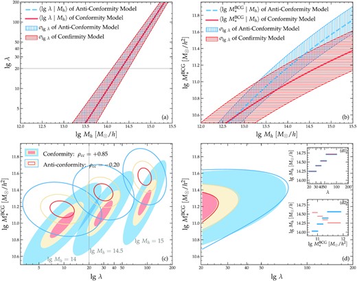
Pedagogical illustration of the degeneracy between conformity (ρcc > 0; red solid curves and filled contours) and anticonformity (ρcc < 0; blue dashed curves and open contours) models of clusters. Panel (a): the mass–richness relations of the two models are exactly the same by design. Panel (b): the stellar-to-halo mass relations of the two models are different, with the conformity model having a shallower slope and larger scatter than the anticonformity model. Panel (c): The three consecutive contours of each model indicate the two-dimensional (2D) PDFs of clusters on the |$M_*^{\texttt {BCG}}$| versus λ plane predicted at fixed log–halo masses of 14, 14.5, and 15 (from left to right), respectively. The differences are not observable due to the lack of individual halo mass measurements. Panel (d): The 2D abundance of clusters on the observed |$M_*^{\texttt {BCG}}$| versus λ plane, predicted by the conformity (filled) and anticonformity (open) models. The inset panels (d1) and (d2) show the average halo mass of clusters in four bins of λ and |$M_*^{\texttt {BCG}}$|, respectively. In each inset panel, thick blue and thin red lines indicate the predictions by the anticonformity and conformity models, respectively. The two sets of model predictions are almost indistinguishable in their 2D abundances (panel d) and halo mass in bins of λ (panel d1), despite the large discrepancies shown in panels (b) and (c). This strong degeneracy can be potentially broken by measuring the halo mass of clusters in bins of |$M_*^{\texttt {BCG}}$| (panel d2).
However, there exists a systematic uncertainty in our central galaxy stellar mass measurement due to the mis-centring effect, i.e. some of the BCGs identified by the maximum pcen are actually satellite galaxies (Zhang et al. 2019). From the weak lensing analysis, Paper I inferred that |${\sim }30{{\ \rm per\ cent}}$| of the redMaPPer clusters in our sample are mis-centred, and the mis-centring fraction decreases with increasing |$M_*^{\texttt {BCG}}$|. To assess the size of the systematic bias induced by mis-centring, we examine the distribution of the stellar mass gaps |$\Delta M_*^{\texttt {BCG}}$| between galaxies with the maximum (i.e. our BCG candidates) and second highest pcen in individual clusters. We find that in |$25{{\ \rm per\ cent}}$| of the clusters the second probable central is more massive than the BCG we select, and that among those clusters with |$\Delta M_*^{\texttt {BCG}}{\lt }0$|, |$70{{\ \rm per\ cent}}$| of them have |$\Delta M_*^{\texttt {BCG}}{\gt }-0.1$| dex. Therefore, assuming that the mis-centred clusters are likely those with negative stellar mass gaps, we expect that the BCG stellar mass of the mis-centred clusters could be systematically underestimated by ∼0.05−0.1 dex.
2.2 Cluster weak lensing measurements
We employ two sets of cluster weak lensing measurements in our analysis. For the Bayesian analysis in Section 4, we derive constraints on |$p(M_*^{\texttt {BCG}}, \lambda |M_\mathrm{ h})$|, the 2D probability density function of the |$M_*^{\texttt {BCG}}$| and λ of clusters at fixed Mh by making use of the weak lensing halo mass measurements of clusters in bins of λ from Simet et al. (2017). In particular, we assume the best-fitting mass–richness relation inferred by Simet et al. (2017) (their equation 28) and compute the mean halo mass in each of the four richness bins, which is listed in Table 1. Following Simet et al. (2017) (also see Costanzi et al. 2019b), we assign 50 per cent of the uncertainties as systematic errors, which we assume to be fully correlated between different richness bins. Murata et al. (2018) showed that the mass–richness relation of Simet et al. (2017) derived from the SDSS imaging is consistent with the recent measurements from the Hyper Suprime-Cam (HSC; Aihara et al. 2018; Mandelbaum et al. 2018). We refer interested readers to Simet et al. (2017) for technical details of the halo mass measurements.
Weak lensing mass estimates (and associated uncertainties) of the redMaPPer clusters binned by λ, derived from Simet et al. (2017). We assume that 50 per cent of the uncertainties are systematic errors.
| λ | [20,30) | [30,40) | [40,55) | [55, 100) |
|---|---|---|---|---|
| |$\lg \, M_\mathrm{ h}$| | 14.05 ± 0.05 | 14.25 ± 0.05 | 14.43 ± 0.05 | 14.64 ± 0.05 |
| λ | [20,30) | [30,40) | [40,55) | [55, 100) |
|---|---|---|---|---|
| |$\lg \, M_\mathrm{ h}$| | 14.05 ± 0.05 | 14.25 ± 0.05 | 14.43 ± 0.05 | 14.64 ± 0.05 |
For testing whether our best-fitting models of |$p(M_*^{\texttt {BCG}}, \lambda |M_\mathrm{ h})$|, in combination with the cluster assembly bias prescription, can resolve the ‘halo mass equality’ conundrum, we predict the surface density contrast profiles ΔΣ(rp) for the low- and high-|$M_*^{\texttt {BCG}}$| cluster subsamples and compare to the weak lensing measurements of the two subsamples made in Paper I from the DECaLS imaging (Dey et al. 2019). We will directly present the comparison in Section 5 and refer the readers to Paper I for technical details of the weak lensing measurements from DECaLS.
Note that we do not include the halo mass estimates for the low- and high-|$M_*^{\texttt {BCG}}$| clusters from Paper I in our Bayesian analysis of Section 4, because the estimates from Paper I do not include some of the systematic uncertainties considered by Simet et al. (2017), including the shear calibration errors, photo-z biases, halo triaxiality, etc. Therefore, to avoid inhomogeneity in our input data, we include only the weak lensing halo mass in bins of λ measured by Simet et al. (2017) in our Bayesian analysis but directly model the ΔΣ measurements from Paper I in Section 5.
3 METHODOLOGY
The data vector of our Bayesian analysis in Section 4 consists of three components:
Ncls = 5476: the total number of clusters observed with λ ≥ 20 and 0.17 < z < 0.30 over a sky area of 10401 deg2.
|$\lbrace M_*^{\texttt {BCG}}, \lambda \rbrace _{i=1 \cdots 5476}$|: BCG stellar mass and satellite richness of the observed 5476 individual clusters.
|$\lbrace M_\mathrm{ h} \mid [\lambda _{\mathrm{min}}^j, \lambda _{\mathrm{max}}^j]\rbrace _{j=1\cdots 4}$|: Weak lensing halo mass measurements of four richness bins listed in Table 1.
Below we will describe our analytic model for predicting each of the three components.
3.1 Modelling the 2D PDF of |$\boldsymbol {M_*^{\texttt {BCG}}}$| and |$\boldsymbol {\lambda }$| at fixed |$\boldsymbol {M_\mathrm{ h}}$|
The 2D PDF of |$M_*^{\texttt {BCG}}$| and λ at fixed Mh, |$p(M_*^{\texttt {BCG}}, \lambda |M_\mathrm{ h})$| is the centrepiece of our statistical model of galaxy–halo connection for clusters. Our model of |$p(M_*^{\texttt {BCG}}, \lambda |M_\mathrm{ h})$| consists of three components, the richness-to-halo–mass relation (RHMR) that describes the one-dimensional (1D) lognormal PDF of richness at fixed halo mass p(λ∣Mh), the stellar-to-halo−mass relation (SHMR) that specifies the 1D lognormal PDF of BCG stellar mass at fixed halo mass |$p(M_*^{\texttt {BCG}}\mid M_\mathrm{ h})$|, and the correlation coefficient between |$M_*^{\texttt {BCG}}$| and λ as a function of halo mass ρcc(Mh). We will refer to models with ρcc > 0 as ‘conformity’ models and those with ρcc < 0 as ‘anticonformity’ models, respectively.
As mentioned in Section 1, Paper I discovered that the scatter of the SHMR is at least partially driven by the concentration of dark matter haloes, so that the more massive BCGs are preferentially hosted by the more concentrated haloes at fixed halo mass. Therefore, to accurately predict the weak lensing profiles of clusters binned by |$M_*^{\texttt {BCG}}$|, we also need to take into account the concentration–bias relation predicted by the halo assembly bias effect, as will be discussed later in Section 5.
3.2 Predicting observing probability of each cluster
3.3 Predicting halo mass distribution of each cluster
4 BAYESIAN INFERENCE: A TALE OF TWO CONFORMITY MODELS
4.1 Model degeneracy: Conformity versus anticonformity
Before moving on to the Bayesian inference of model parameters, we illustrate in Fig. 1 that there exists a strong degeneracy in our current model so that both conformity and anticonformity models can describe the 2D abundance of clusters and the weak lensing halo mass in bins of richness, with exactly the same RHMR but different SHMRs.
In the top left-hand panel of Fig. 1, the red solid and blue dashed lines are the mean RHMRs of the conformity and anticonformity models, respectively, with horizontally and vertically hatched bands of the same colours indicating their corresponding scatters. The two RHMRs are exactly the same by design, so that the two models will predict exactly the same average halo mass for any cluster sample binned in richness (as shown in panel d1). The minimum richness cut of 20 is indicated by the grey horizontal line. In the top right-hand panel of Fig. 1, we adopt the same plotting styles for the conformity versus anticonformity models as in the top left-hand panel but show the SHMRs instead. The SHMR of the conformity model (red solid line with horizontally hatched band) has a shallower slope but a larger scatter than that of the anticonformity model (blue dashed line with vertically hatched band). As a result, the two models will predict different average halo masses for clusters selected by the BCG stellar mass (as shown in panel d2).
In the bottom left-hand panel of Fig. 1, filled and open contours indicate the 2D PDFs of |$M_*^{\texttt {BCG}}$| and λ at three fixed halo masses of |$\lg \, M_\mathrm{ h}{=}14$|, 14.5, and 15, of the conformity (ρcc = 0.85) and anticonformity (ρcc = − 0.2) models, respectively. Each contour has three levels at |$20{{\ \rm per\ cent}}$| (red), |$50{{\ \rm per\ cent}}$| (beige), and |$90{{\ \rm per\ cent}}$| (blue) enclosed probabilities expanding outwards. Unsurprisingly, the two models yield two drastically different |$p(\ln M_*^{\texttt {BCG}}, \ln \lambda \mid M_\mathrm{ h})$| at every mass. Yet, the 2D abundance of clusters on the |$M_*^{\texttt {BCG}}$| versus λ diagram (bottom right-hand panel) predicted by the two models are strikingly similar — the filled (conformity) and open (anticonformity) contours are mostly aligned and overlapping, leaving little observational signature to distinguish the two models from 2D abundance alone. In the two inset panels, we show the average halo mass of clusters in bins of λ (panel d1) and |$M_*^{\texttt {BCG}}$| (panel d2), respectively. As expected, the halo masses are exactly the same when binned by λ, as a result of the RHMRs being the same. Therefore, if we constrain conformity using just the 2D abundance and halo mass in bins of λ, there would be a strong degeneracy between the conformity and anticonformity models, as will be demonstrated later in Section 4.1.
However, the two sets of predicted halo mass in bins of |$M_*^{\texttt {BCG}}$| are significantly different. The conformity model predicts that the average halo mass is a decreasing function of |$M_*^{\texttt {BCG}}$|, while the anticonformity model predicts an increasing trend with |$M_*^{\texttt {BCG}}$|. This discrepancy is likely related to the ‘halo mass equality’ conundrum discovered in Paper I, showing that the halo mass trend with |$M_*^{\texttt {BCG}}$| could be highly non-trivial and depends critically on the level of conformity within the cluster sample. More important, the strong discrepancy shown in the panel d2 of Fig. 1 implies that the halo mass measurements for the low- and high-|$M_*^{\texttt {BCG}}$| subsamples from Paper I could be the key in breaking the degeneracy between the two types of conformity models, as will be shown later in Section 4.4. Note that the predictions of halo mass as a function of stellar mass shown in panel d2 (and throughout this paper) are for central galaxies of clusters with λ ≥ 20 and therefore cannot be directly compared with the measurements for central galaxies of all haloes (Mandelbaum et al. 2016; Zu & Mandelbaum 2016).
4.2 Likelihood model
To summarize our model parameters |$\boldsymbol {\theta }$| from Section 3, we have in total 12 free parameters, including {A, α, σln λ, 0, q} for describing the RHMR, |$M_{\mathrm{ h}, 1}, \lbrace M_{*,0}, \beta , \delta , \gamma , \sigma _{\ln M_*^{\texttt {BCG}}\mid M_\mathrm{ h}}\rbrace$| for describing the SHMR, and {ρcc, 0, s} for describing the sign and level of the BCG-satellite conformity.
Since β and γ describe the low-to-intermediate-mass portion of the SHMR, which is largely irrelevant to our constraint in the cluster mass regime, we apply two Gaussian priors informed by the constraint from Zu & Mandelbaum (2015) using the galaxy clustering and galaxy–galaxy lensing measurements from SDSS: |$\beta {\sim }\mathcal {N}(0.33, 0.18^2)$| and |$\gamma {\sim }\mathcal {N}(1.21, 0.19^2)$|, respectively. For the rest of the parameters, we assume uniform priors so that each parameter could vary freely within a range that is much larger than potentially allowed by the data.
To recap our data vector from Section 2, we have measured the total number of observed clusters Ncls, the BCG stellar mass and satellite richness of individual clusters |$\lbrace M_*^{\texttt {BCG}}, \lambda \rbrace _{i=1 \cdots N_{\mathrm{cls}}}$|, and the average halo mass of clusters binned in richness |$\lbrace M_\mathrm{ h} \mid [\lambda _{\mathrm{min}}^j, \lambda _{\mathrm{max}}^j]\rbrace _{j=1\cdots 4}$|. We will describe the likelihood model for each of the three components in turn below.
4.3 Parameter constraint
Equipped with the full likelihood model, we now set out to infer the joint posterior distribution of the 12 model parameters. We first perform the analysis by allowing ρcc, 0 to vary freely between −1 and 1, yielding a dominant solution that prefers a positive ρcc, 0 (i.e. conformity), as well as a secondary solution with ρcc, 0 < 0 (i.e. anticonformity). This model degeneracy is expected from our simple experiment in Section 4.1. To thoroughly explore the two solutions separately, we then repeat our inference twice by first limiting ρcc, 0 ∈ [0, 1) and then ρcc, 0 ∈ (− 1, 0] when sampling the posterior distributions, yielding a best-fitting conformity and an anticonformity model, respectively. Since we will be distinguishing the two degenerate solutions using the weak lensing of clusters binned by |$M_*^{\texttt {BCG}}$| in Section 4.4, we present the two solutions in parallel below without comparing their relative statistical significance.
For each inference, we employ the affine invariant Markov Chain Monte Carlo (MCMC) ensemble sampler emcee (Foreman-Mackey et al. 2013). We run the MCMC sampler for 2 000 000 steps for each analysis to ensure its convergence and derive the posterior constraints after a burn-in period of 500 000 steps. The median values and the 68 per cent confidence limits of the 1D posterior constraints are listed in Table 2.
Posterior constraints of the model parameters for the two models. The uncertainties are the |$68\%$| confidence regions derived from the 1D posterior probability distributions.
| Parameters | Conformity model | Anticonformity model |
|---|---|---|
| A | |$3.44_{-0.03}^{+0.03}$| | |$3.41_{-0.03}^{+0.03}$| |
| α | |$1.06_{-0.03}^{+0.03}$| | |$0.96_{-0.02}^{+0.03}$| |
| |$\ln \, M_{\mathrm{ h},1}$| | |$21.83_{-2.18}^{+2.60}$| | |$22.82_{-2.10}^{+1.97}$| |
| |$\ln \, M_{*,0}$| | |$20.57_{-1.13}^{+1.20}$| | |$20.23_{-1.36}^{+1.31}$| |
| β | |$0.35_{-0.15}^{+0.18}$| | |$0.42_{-0.17}^{+0.18}$| |
| δ | |$0.30_{-0.04}^{+0.05}$| | |$0.24_{-0.03}^{+0.03}$| |
| γ | |$1.21_{-0.19}^{+0.19}$| | |$1.20_{-0.19}^{+0.20}$| |
| |$\sigma _{\ln \, \lambda ,\, 0}$| | |$0.32_{-0.04}^{+0.03}$| | |$0.39_{-0.03}^{+0.03}$| |
| q | |$-0.20_{-0.03}^{+0.02}$| | |$-0.13_{-0.02}^{+0.01}$| |
| |$\sigma _{\ln \, M_*}$| | |$0.40_{-0.10}^{+0.09}$| | |$0.28_{-0.09}^{+0.10}$| |
| |$\rho _{\mathrm{ cc},\, 0}$| | |$0.60_{-0.23}^{+0.17}$| | |$-0.48_{-0.22}^{+0.24}$| |
| s | |$0.08_{-0.06}^{+0.05}$| | |$-0.12_{-0.05}^{+0.06}$| |
Fig. 2 compares the two separate parameter constraints derived for the conformity (red) and anticonformity (blue) models. For each model, the histograms in the diagonal panels show the 1D marginalized posterior distributions of each of the 12 parameters, and the contours in the off-diagonal panels are the |$50{{\ \rm per\ cent}}$| and |$90{{\ \rm per\ cent}}$| confidence regions for each of the parameter pairs. The grey solid line running through the ρcc, 0-related panels divides the conformity versus anticonformity models at ρcc, 0 = 0. In the top right corners, we provide a brief description of the functionality of each model parameter within each of the three components of our |$p(\ln M_*^{\texttt {BCG}}, \ln \lambda \mid M_\mathrm{ h})$| model (i.e. RHMR, SHMR, and BCG-satellite conformity).
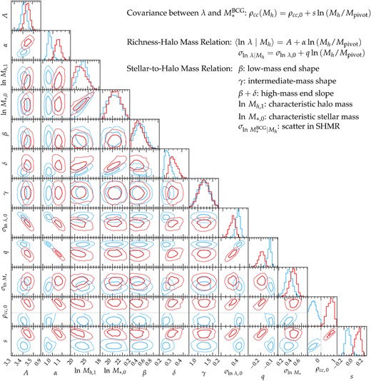
Parameter constraints of the conformity (red) and anticonformity (blue) models. Diagonal panels show the 1D posterior distributions of each of the 12 parameters, while the off-diagonal panels indicate the 2D confidence regions (50 per cent and 90 per cent from inside out) of the constraint on each of the parameter pairs. Grey dashed curves in the diagonal panels of β and γ are the Gaussian prior distributions. A short description of each parameter is given by the legend in the top right corner.
Fig. 3 compares the predictions from the conformity (red) and anticonformity (blue) posterior mean models to the data. The orange dots in the left-hand panel represent the observed cluster distribution on the |$M_*^{\texttt {BCG}}$| versus λ diagram, with the three thick grey dashed contour lines enclosing 20, 50, and 90 percentiles of the cluster sample (from the inside out), respectively. Red solid and blue dashed contour lines indicate the same three levels in percentiles predicted by the conformity and anticonformity posterior mean models. Both models provide adequate descriptions of the underlying 2D distributions of clusters on the |$M_*^{\texttt {BCG}}$| versus λ diagram. The right-hand panel of Fig. 3 compares the weak lensing-measured halo masses in four bins of richness (open circles with error bars) to those predicted by the conformity (red triangles) and anticonformity (blue inverted triangles) posterior mean models. Both model predictions are in good agreement with the weak lensing mass measurements, with the (anti-)conformity model predictions slightly lower (higher) than the observations at the low-richness end. Overall, Fig. 3 confirms our expectation from Fig. 1 that there exists a model degeneracy that cannot be overcome by the combination of 2D cluster abundance and halo mass measurements in bins of richness.
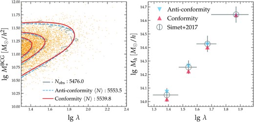
Comparison between the data and the predictions from the posterior mean parameters of the conformity (red solid) and anticonformity (blue dashed) model constraints. Left: 2D PDFs of clusters on the |$M_*^{\texttt {BCG}}$| and λ plane. Grey dot–dashed contours and yellow points indicate the observed PDFs and individual clusters, respectively. The total number of observed and predicted clusters are marked by the legend in the bottom right. Right: average log-halo mass in four bins of richness. Open circles with error bars are the measurements from Simet et al. (2017), and red and blue triangles indicate the posterior mean predictions from the conformity and anticonformity models, respectively. Both models provide good fits to the data.
Fig. 4 provides a more visually appealing way of comparing the two model constraints. Instead of showing the posterior distributions of the 12 individual parameters, we examine the behaviours of the best-fitting RHMRs (left), BCG-satellite conformities (middle), and SHMRs (right), respectively. In the left-hand panel, we also show the mean RHMRs derived by Murata et al. (2018) (grey dot dashed) and Costanzi et al. (2019b) (grey dotted) for the SDSS redMaPPer clusters. Unsurprisingly, the RHMRs predicted by the conformity (red solid) and anticonformity (blue dashed) models are reasonably similar at λ ≥ 20, because they are primarily constrained by the observed abundance and average halo mass of clusters binned in richness, which are independent of ρcc(Mh). The shaded band about each mean RHMR indicates the dependence of scatter on halo mass. Compared to the Murata et al. (2018) result, our RHMRs have a higher amplitude but the same slope, likely due to a slight shift in the weak lensing halo mass calibration compared to ours – they used the shear catalogue from the HSC survey and a cluster sample with z ∈ [0.1, 0.33]. The RHMR derived by Costanzi et al. (2019b) has a much shallower slope than the other three, because they also varied cosmology while inferring the RHMR.
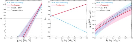
Mass–richness relation (left), correlation coefficient variation (middle), and stellar-to-halo mass relation (right), predicted by the conformity (red solid) and anticonformity (blue dashed) posterior mean models. Dotted and dot–dashed lines in the left-hand panel indicate the best-fitting models from Costanzi et al. (2019b) and Murata et al. (2018), respectively. In the right-hand panel, dotted and dot–dashed curves are the best-fitting models from Guo, Yang & Lu (2018) and Zu & Mandelbaum (2015), respectively. Shaded bands in the left-hand and right-hand panels indicate the 1 − σ logarithmic scatter about the median scaling relations.
In the right-hand panel of Fig. 4, we compare the SHMRs inferred from the conformity (red solid) and anticonformity (blue dashed) models, as well as the results from Zu & Mandelbaum (2015) (grey dot-dashed) using the galaxy clustering and galaxy–galaxy lensing at z ∼ 0.1 and from Guo et al. (2018) (grey dotted) using the LOWZ galaxy clustering at the same redshift of our sample. Unlike the RHMRs, our two inferred SHMRs are significantly different, with the conformity SHMR showing a shallower slope but a larger scatter than the anticonformity one. Additionally, the result from Guo et al. (2018) is consistent with the conformity constraint, while the Zu & Mandelbaum (2015) curve has a similar slope but a higher amplitude compared to the conformity prediction, probably due to some redshift evolution of the SHMR from z ∼ 0.25 to 0.1. Both the Guo et al. (2018) and Zu & Mandelbaum (2015) constraints are strongly inconsistent with the prediction by the anticonformity model.
Finally, the middle panel of Fig. 4 shows the correlation coefficients as functions of halo mass ρcc(Mh), predicted by the conformity (red solid) and anticonformity (blue dashed) models, respectively. Interestingly, both predictions favour a weak correlation between the BCG stellar mass and satellite richness at the low-mass end (i.e. below |$10^{13}\, h^{-1}M_{\odot }$|) but bifurcate into strong positive and negative correlations at the high-mass end (i.e. above a few times |$10^{14}\, h^{-1}M_{\odot }$|). The two different scenarios point to drastically different paths of galaxy formation within massive clusters – the conformity model implies a correlated growth between the BCG and satellite galaxies, while the anticonformity model favours a compensated growth between the two galaxy populations. Therefore, it is vital to observationally distinguish the two scenarios for a better understanding of the underlying physics behind cluster galaxy formation.
4.4 Resolving the ‘halo mass equality’ conundrum
As mentioned in the introduction, we are hopeful that the existence of a strong (anti-)conformity between the BCG stellar mass and satellite richness could potentially reconcile the ‘halo mass equality’ conundrum – that is, when split into two halves by the median |$M_*^{\texttt {BCG}}$| at fixed λ, the two cluster subsamples have almost the same average halo mass, despite having a 0.34-dex discrepancy in their average |$M_*^{\texttt {BCG}}$|. We refer readers to Paper I for details on the subsample definition (see also Fig. 5) and the original ‘halo mass equality’ conundrum. We now explore whether one of the two posterior mean models we inferred in Section 4.3 is consistent with such ‘halo mass equality’ phenomenon.
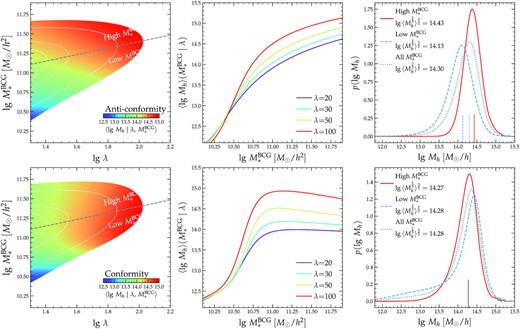
Predictions of halo mass distributions by the anticonformity (top row) and conformity (bottom row) posterior mean models. In each row, the left-hand panel shows the map of average log-halo mass on the |$M_*^{\texttt {BCG}}$| versus λ plane, colour-coded by the horizontal colour bar in the bottom right corner. Grey dashed line indicates the median log-|$M_*^{\texttt {BCG}}$| versus λ relation, which divides the clusters into two subsamples of high and low |$M_*^{\texttt {BCG}}$| with the same distribution of λ. The middle panel shows the variation of log-Mh as a function of |$M_*^{\texttt {BCG}}$| at four fixed values of λ of 20 (purple), 30 (cyan), 50 (yellow), and 100 (red), respectively. The right-hand panel compares the PDFs of log-Mh of the high-|$M_*^{\texttt {BCG}}$| (red solid) and low-|$M_*^{\texttt {BCG}}$| (blue dashed) subsamples, as defined in the left-hand panel, with the PDF of all the clusters shown by the grey dotted curve. The predicted average weak lensing halo mass of each cluster (sub)sample is marked by the bottom vertical tick of the respective line colour/style and shown in the legend. The two models predict significantly different halo masses for the high- and low-|$M_*^{\texttt {BCG}}$| subsamples, despite reproducing the similar observables in Fig. 3.
Fig. 5 illustrates the differences between the anticonformity (top row) and conformity (bottom row) models in decomposing the underlying halo mass distribution of the high- and low-|$M_*^{\texttt {BCG}}$| subsamples. In each row, the left-hand panel shows the variation of the average halo mass across the |$M_*^{\texttt {BCG}}$| versus λ plane, with the logarithmic mass indicated by the colour bar in the bottom right. The grey dashed line represents the median |$M_*^{\texttt {BCG}}$|–λ relation that splits the clusters into high- and low-|$M_*^{\texttt {BCG}}$| subsamples in Paper I. Interestingly, the high-|$M_*^{\texttt {BCG}}$| clusters have on average higher halo masses than the low-|$M_*^{\texttt {BCG}}$| systems in the anticonformity scenario (top left), while the trend of average halo mass with |$M_*^{\texttt {BCG}}$| is less clear in the conformity model (bottom left). We further clarify the halo mass trend with |$M_*^{\texttt {BCG}}$| in the middle panels by showing the average log-halo mass as functions of |$M_*^{\texttt {BCG}}$| at four different richnesses of 20 (purple), 30 (green), 50 (yellow), and 100 (red), respectively. Clearly, all the four curves are monotonic with |$M_*^{\texttt {BCG}}$| in the anticonformity model but exhibit a plateau above |$M_*^{\texttt {BCG}}{\sim }10^{11}h^{-2}M_{\odot }$| in the conformity model. Note that the plateau is a unique feature predicted by the conformity and cannot be mimicked by systematic effects like the mis-centring, which primarily affects the low-|$M_*^{\texttt {BCG}}$| systems.
The right-hand panels of Fig. 5 provide the key to potentially resolving the ‘halo mass equality’ conundrum. In each panel, we show the underlying halo mass distributions for all (grey dotted), low-|$M_*^{\texttt {BCG}}$| (blue dashed), and high-|$M_*^{\texttt {BCG}}$| (red solid) clusters, respectively. Additionally, we indicate the average weak lensing halo mass (|$\langle M_\mathrm{ h}^{2/3} \rangle ^{3/2}$|; see Mandelbaum et al. 2016) of each of the three distributions using a short vertical line of the same colour at the bottom. Unsurprisingly, the two subsamples are predicted to have an ∼0.3-dex discrepancy in their average weak lensing halo mass in the anticonformity model (top right), due to the monotonic trend of halo mass with |$M_*^{\texttt {BCG}}$| across the entire richness range.
However, in the bottom right-hand panel of Fig. 5, the conformity model predictions exhibit exactly the same ‘halo equality’ as discovered in Paper I – the two subsamples of clusters have almost the same weak lensing halo mass, despite the significant difference in the shape of their halo mass distributions. In particular, the conformity model predicts a stronger low-Mh tail and a more massive peak for the halo mass distribution of the low-|$M_*^{\texttt {BCG}}$| subsample than the high-|$M_*^{\texttt {BCG}}$| one. More important, the low-Mh tail and the high-Mh peak somehow conspire to produce an average weak lensing halo mass that is very similar to that of the high-|$M_*^{\texttt {BCG}}$| clusters, thereby resolving the ‘halo mass equality’ conundrum of Paper I.
The average halo mass estimated by Paper I for the low- and high-|$M_*^{\texttt {BCG}}$| subsamples is |$\lg M_\mathrm{ h}{=}14.24{\pm }0.02$|, roughly |$10{{\ \rm per\ cent}}$| lower than predicted by the best-fitting conformity model (14.28). However, as mentioned in Section 2.2, the estimated uncertainty of halo mass (±0.02 dex) in Paper I does not include many of the systematic uncertainties that were included by Simet et al. (2017) and therefore should be considered a lower limit. If we assume the typical mass error of 0.05 dex from Simet et al. (2017), e.g. by adding an extra 0.03 dex of fully correlated systematic error, the two sets of halo mass estimates would be consistent within 1σ. In the future, we can further tighten the constraints on conformity by applying a uniform halo mass measurement method to clusters binned by |$M_*^{\texttt {BCG}}$| and λ.
Before moving on to the second half of the paper, we summarize our key results so far as follows.
We have inferred the best-fitting models under different assumptions of conformity versus anticonformity between the BCG stellar mass and the satellite richness, using the combination of cluster abundance and weak lensing mass of clusters binned in λ as constraints.
Both best-fitting conformity and anticonformity models provide good descriptions of the data, but they predict significantly different average halo masses for clusters binned in |$M_*^{\texttt {BCG}}$|.
By comparing to the weak lensing halo mass measurements of the low- and high-|$M_*^{\texttt {BCG}}$| clusters, we demonstrated that while the anticonformity model is strongly disfavoured by the data, the best-fitting conformity model predicts the same average halo mass for the two cluster subsamples, thereby resolving the ‘halo mass equality’ conundrum discovered by Paper I (Fig. 5).
5 MODELLING CLUSTER WEAK LENSING WITH CONFORMITY AND ASSEMBLY BIAS
Apart from the ‘halo mass equality’ conundrum that we focused on in the first part of this paper, Paper I also discovered that the low-|$M_*^{\texttt {BCG}}$| clusters on average exhibit a |$20{{\ \rm per\ cent}}$| lower concentration (5.87 versus 6.95) and an |${\sim }10{{\ \rm per\ cent}}$| higher large-scale bias than their low-|$M_*^{\texttt {BCG}}$| counterparts. Paper I suggested that the bias discrepancy could be an evidence of cluster assembly bias (Zu et al. 2017). However, while the concentration measurements from the small-scale weak lensing profiles are robust (modulo the degeneracy with the cluster mis-centring effect), the modelling of large-scale biases in Paper I is lacking, due to the omission of the halo assembly bias effect that governs the concentration–bias relation of clusters at fixed Mh.
Therefore, in the second part of this paper, we will implement halo assembly bias in our posterior mean conformity model inferred from Section 4.3, in order to provide a more accurate model for the weak lensing profiles ΔΣ which can then be compared with the measurements for the low- and high-|$M_*^{\texttt {BCG}}$| subsamples from Paper I.
To avoid distracting the impatient, we will directly present the ΔΣ predictions from our best-fitting analytic models that include the halo assembly bias and (anti-)conformity in this section. For those who are interested in the modelling details, we describe the calibration and prescription of halo assembly bias in Appendix Section A, and the analytic model of weak lensing profiles in Appendix Section B.
5.1 Fitting to weak lensing of high- and low-|$\boldsymbol {M_*^{\texttt {BCG}}}$| clusters
Fig. 6 compares the stacked weak lensing measurements to those predicted by the posterior mean anticonformity model (left column), conformity model without assembly bias (middle column), and conformity model with assembly bias (right column), respectively. The top and bottom rows are the same except for the labels of the y-axes (ΔΣ versus rpΔΣ). In each panel, red circles and blue squares are the weak lensing measurements of the high- and low-|$M_*^{\texttt {BCG}}$| subsamples (same as those shown in fig. 5 of Paper I), respectively, while red solid and blue dashed curves are the respective model predictions. The values of average concentration 〈c〉 and average bias 〈b〉 adopted by each model are indicated in the top right of each top panel. Unsurprisingly, the predictions by the anticonformity model in the left-hand panels fail to describe the ΔΣ measurements on all scales, due to the factor of 2 difference between the two predicted average halo masses and the |${\sim }30{{\ \rm per\ cent}}$| discrepancy between the two predicted biases.
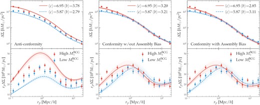
Comparison between the surface density contrast profile ΔΣ measured by Paper I from weak lensing and that predicted by three different models: anticonformity (left column), conformity without assembly bias (middle column), and conformity with assembly bias (right column). In each column, the top and bottom panels show the same information except that the y-axis of the bottom panel is rpΔΣ. In each panel, red circles and blue squares with error bars are the weak lensing measurements for the high- and low-|$M_*^{\texttt {BCG}}$| subsamples, respectively. Red solid and blue dashed thick curves are the predictions from the respective posterior mean model, while the bundle of thin curves around each thick curve is predicted from 100 random steps along the respective MCMC chain from Fig. 2. The values of average concentration and bias adopted by each model are listed in the top right corner of each column. For the ΔΣ prediction, we adjust the average halo concentrations to be the best-fitting values inferred from Paper I on small scales but predict the large-scale bias using different prescriptions (see text for details).
In the middle panels of Fig. 6, the conformity-only (i.e. without assembly bias) model provides good description of the small-scale ΔΣ measurements, echoing the finding in Fig. 5 that the average weak lensing halo masses of the two subsamples are similar. On large scales, the two predicted ΔΣ profiles converge to the same amplitudes, because the similar average halo masses produce similar biases in the absence of assembly bias. In the right-hand panels of Fig. 6, the small-scale behaviour of the ΔΣ profiles predicted by the conformity + AB (i.e. with assembly bias) model is the same as in the middle panels, but on large scales, the two predicted curves differ by about |$10{{\ \rm per\ cent}}$| – the high-|$M_*^{\texttt {BCG}}$| clusters are more concentrated, producing a lower bias than the low-|$M_*^{\texttt {BCG}}$| systems due to the cluster assembly bias effect.
Due to the relatively large error bars of ΔΣ on large scales, it is difficult to ascertain whether the conformity + AB model is superior to the conformity-only model. Therefore, we further examine the large-scale behaviours of the three models in Fig. 7, where we show the projected cross-correlation functions between clusters and LOWZ galaxies (left) and the cluster galaxy number density profiles measured from the cross-correlations with photometric galaxies (right). Although we cannot directly measure the cluster biases directly from the cross-correlations with galaxies, which also depend on the bias of the galaxies (Xu et al. 2021), we can distinguish the three models by examining the ratio between the cross-correlations of the high- and low-|$M_*^{\texttt {BCG}}$| with galaxies, which is a direct measure of b+/b− independent of galaxy bias.
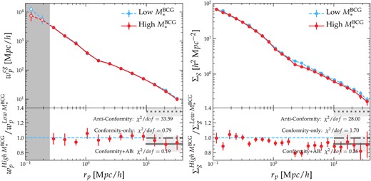
Left-hand panel: Comparison of the projected correlation functions |$w_\mathrm{ p}^{\mathrm{ cg}}$| of the low (blue) and high (red) |$M_*^{\texttt {BCG}}$| subsamples with the BOSS LOWZ spectroscopic galaxy sample in the upper sub-panel, with the ratio of the two shown in the bottom sub-panel. The grey shaded region on the left indicates the distance scales that are affected by the fibre collision in BOSS. Right-hand panel: Similar to the left-hand panel but for the excess galaxy surface number density profile Σg calculated from the SDSS DR8 imaging. In each sub-panel, the bias ratios predicted by the anticonformity, conformity-only (i.e. without assembly bias), and conformity + AB (i.e. with assembly bias) models are indicated by the grey horizontal dotted, dot–dashed, and solid lines on scales above 10h−1Mpc, respectively. The grey shaded band around each horizontal line indicates the 1σ uncertainty predicted by the constraints from Fig. 2.
In each panel of Fig. 7, red and blue circles with error bars indicate the measurements for the high and low-|$M_*^{\texttt {BCG}}$| subsamples, respectively. In the bottom sub-panel, red circles are the ratio between the measurements of the two subsamples. The grey shaded region in the left-hand panel indicates the projected distances that are affected by the fibre collision in BOSS. Fig. 7 is the same as the fig. 6 of Paper I, except that we mark the large-scale ratios predicted by the anticonformity (dotted horizontal line), conformity-only (dot–dashed), and conformity + AB (solid) models in the bottom sub-panels. Clearly, the anticonformity prediction is ruled out by the data. The conformity-only prediction without assembly bias is also disfavoured by the observations, which exhibit a |$10{{\ \rm per\ cent}}$| bias discrepancy between the two subsamples. Meanwhile, the direction and amplitude of this bias discrepancy are in good agreement with the prediction by the conformity model with assembly bias. This is very reassuring – the combination of BCG-satellite conformity and cluster assembly bias not only predicts the correct weak lensing masses of clusters selected by |$M_*^{\texttt {BCG}}$|, therefore resolving the intriguing conundrum discovered in Paper I, but also accurately reproduces the large-scale bias inversion with |$M_*^{\texttt {BCG}}$| using the cluster assembly bias model directly predicted by the ΛCDM simulations.
5.2 Exploring projection effects
The projection effects in photometric cluster detection could induce systematic errors in the cluster observables that could sometimes masquerade as physical phenomena (Busch & White 2017; Zu et al. 2017). As mentioned in the introduction, To et al. (2020) discussed the possibility of projection effects to induce a positive correlation between BCG luminosity and richness by enhancing the estimated richness in the dense environments that potentially host older and more luminous BCGs at fixed halo mass. If the project effects are indeed the culprit, we should expect some correlation between the BCG stellar mass and the level of cluster membership contamination due to projection effects.
We first examine the distributions of the low- and high-|$M_*^{\texttt {BCG}}$| clusters on the Rmem versus λ plane, which is shown on the left-hand panel of Fig. 8. Red and blue contours indicate the |$20{{\ \rm per\ cent}}$|, |$50{{\ \rm per\ cent}}$|, and |$90{{\ \rm per\ cent}}$| enclosed regions, while the red circles and blue squares with error bars show the median Rmem as functions of λ for the high- and low-|$M_*^{\texttt {BCG}}$| subsamples, respectively. The two sets of contours and median relations are well aligned, showing no systematic offset between the high- and low-|$M_*^{\texttt {BCG}}$| subsamples in Rmem. The solid black line is a fit to the median relations that we use to divide each |$M_*^{\texttt {BCG}}$|-based subsample into low- and high-Rmem quarter samples for the test on the right-hand panel.
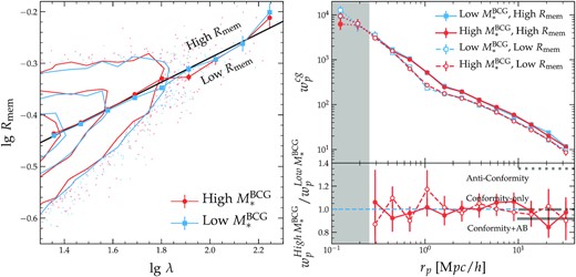
Impact of projection effects on the detection of conformity and assembly bias, using the average member galaxy distance Rmem as a proxy for the strength of projection effects. Left: Distributions of low (blue) and high (red) |$M_*^{\texttt {BCG}}$| clusters on the Rmem versus λ plane. Each set of contour lines indicates the |$20{{\ \rm per\ cent}}$|, |$50{{\ \rm per\ cent}}$|, and |$90{{\ \rm per\ cent}}$| enclosed regions from the inside out. Red circles and blue squares show the median Rmem at fixed λ of the low- and high-|$M_*^{\texttt {BCG}}$| subsamples, with the error bars indicating the uncertainties on the median. The solid black line is a power-law fit to the two median relations, dividing the clusters into low- and high-Rmem populations. Right: Similar to the left-hand panel of Fig. 7 but for subsamples further split by Rmem. We do not detect any significant dependence of |$M_*^{\texttt {BCG}}$| or bias ratio on Rmem.
The right-hand panel of Fig. 8 is similar to the left-hand panel of Fig. 7, except for that we divide each of the low- and high-|$M_*^{\texttt {BCG}}$| subsamples in half based on the solid black line in the left-hand panel and calculate the ratios between the high- and low-|$M_*^{\texttt {BCG}}$| signals within each Rmem half in the bottom right-hand panel. Filled and open red circles (blue squares) indicate the measurements for the high- and low-Rmem quarter samples split from the high (low)-|$M_*^{\texttt {BCG}}$| subsample, respectively. The high-Rmem profiles exhibit enhanced clustering on all scales above 400 h−1kpc than the low-Rmem ones due to strong projection effects, echoing the findings in Sunayama et al. (2020). However, the amplitudes of the relative enhancement are the same between the low- and high-|$M_*^{\texttt {BCG}}$| subsamples, indicating similar projection effects in the high-Rmem clusters regardless of the BCG stellar mass.
Despite the strong projection effects of the high-Rmem clusters, the ratio profiles in the bottom panels are both in good agreement with the prediction from the conformity + AB model as in Fig. 7, though they are also consistent with the prediction from the conformity-only model due to the large uncertainties. Therefore, using the average radius of the member galaxy candidates Rmem as a proxy of the projection effect, we do not find any correlation between projection effect and BCG stellar mass that could induce the strong conformity we detected among the SDSS clusters, nor do we find any evidence that our detected cluster assembly bias signal depends on the level of projection effects within the sample.
6 PHYSICAL IMPLICATIONS
6.1 Could dry mergers drive the strong BCG-satellite conformity?
The physical conformity between the BCG stellar mass and satellite richness implies a correlated growth between the BCGs and satellite galaxies inside clusters, and the increasing trend of ρcc with Mh suggests that the BCGs in the most massive haloes almost grow in lockstep with the accretion of satellite galaxies. This strong conformity could naturally occur if a significant fraction of the BCG stellar mass growth is ex situ, via the dry mergers with massive satellite galaxies that were transported to the cluster centre by dynamical friction (Chandrasekhar 1943; White 1976). Indeed, observations indicate that the mode of BCG stellar mass growth switched from in situ star formation to ex situ stellar accretion around z ∼ 1 (Webb et al. 2015; Lavoie et al. 2016; McDonald et al. 2016; Vulcani et al. 2016; Groenewald et al. 2017; Zhao et al. 2017).
In order for dry mergers to drive a correlated scatter between BCG stellar mass and satellite richness, the merger-induced stellar growth should be significant, e.g. comparable with the intrinsic scatter in the cluster SHMR of ∼0.05−0.1 dex (Golden-Marx et al. 2021). Observationally, the stellar growth from dry mergers since z ∼ 1 varies between |$30{{\ \rm per\ cent}}$| (Collins et al. 2009; Bundy et al. 2017; Lin et al. 2017) and almost a factor of 2 (Whiley et al. 2008; Burke & Collins 2013; Lidman et al. 2013). However, semi-analytic models (SAMs) predict that the BCG stellar mass could grow by a factor of 3–4 between z = 1 and z = 0 (De Lucia & Blaizot 2007; Ruszkowski & Springel 2009; Laporte et al. 2013; Oogi, Habe & Ishiyama 2016). The discrepancy between SAM predictions and observations is partly due to the numerical uncertainties in modelling dynamical friction (Boylan-Kolchin, Ma & Quataert 2008; Jiang et al. 2008), and it is also unclear what fraction of the accreted stars would end up in the diffuse intracluster light (Murante et al. 2007; Contini, Yi & Kang 2018).
Alternatively, using a self-consistent model of the observed conditional stellar mass functions across cosmic time, Yang et al. (2013) carefully accounted for the total amount of in situ growth by modelling the star formation histories of central galaxies as a function of halo mass, stellar mass, and redshift. Their indirect method estimated that at z ≥ 2.5 less than 1 per cent of the stars in the progenitors of massive galaxies are formed ex situ, but this fraction increases rapidly with redshift, becoming ∼40 per cent at z = 0. Therefore, by combining the observations, SAM predictions, and indirect estimates, we expect the average amount of merger-induced stellar mass growth to be between 0.1 and 0.3 dex, hence more than enough for driving a correlated scatter with richness.
Finally, the observed richness roughly corresponds to the number of massive, quenched satellite galaxies in each cluster, i.e. the same type of galaxies that would preferentially merge with the BCG within a Hubble time. For instance, Boylan-Kolchin et al. (2008) estimated that roughly |$10{-}20{{\ \rm per\ cent}}$| of all the accreted satellites with mass ratio above 1:10 would merge with the BCG within 7 Gyr due to dynamical friction (see also Jiang et al. 2008). As a result, the observed conformity between BCG stellar mass and richness could be strongly boosted by the fact that the low-mass, star-forming satellites are often not included when calculating the richness of optical clusters.
6.2 Is BCG-satellite conformity consistent with the |$\boldsymbol {c}-\boldsymbol {M_*^{\texttt {BCG}}}$| and |$\boldsymbol {c}-\boldsymbol {\lambda }$| relations?
Paper I showed that halo concentration is one of the key drivers of scatter in the SHMR of clusters, so that clusters with more concentrated cores host more massive BCGs at fixed halo mass – a positive |$c{-}M_*^{\texttt {BCG}}$| correlation. In Paper I, we speculated that the correlation between c and |$M_*^{\texttt {BCG}}$| is caused by the fact that the in situ stellar mass growth of the BCGs is closely tied to the rapid growth of dark matter mass at early times. At the onset of cluster formation, fast accretion and frequent mergers not only built up the central cores of dark matter haloes (Zhao et al. 2003; Klypin et al. 2016) but also drove strong starbursts in the progenitors of the BCGs via rapid cooling flows and shocks, respectively (Barnes & Hernquist 1991; Fabian 1994; Mihos & Hernquist 1996; McDonald et al. 2012; Hopkins et al. 2013).
Meanwhile, there exists a well-known anticorrelation between the concentration and substructure abundance of haloes at fixed halo mass (Giocoli et al. 2010), which should translate to a c − λ anticorrelation at fixed Mh. Combining this anticorrelation with the positive correlation between c and |$M_*^{\texttt {BCG}}$|, one might naively expect that the clusters with high λ (hence low c) would host less-massive BCGs than their low-λ counterparts at fixed Mh – an anticonformity between |$M_*^{\texttt {BCG}}$| and λ, in apparent contradiction with our finding of a strong BCG-satellite conformity from the data.
6.3 A toy model for the |$\boldsymbol {M_*^{\texttt {BCG}}}-\boldsymbol {\lambda }-\boldsymbol {c}$| relation at fixed |$\boldsymbol {M_\mathrm{ h}}$|
The key to understanding the connection between |$M_*^{\texttt {BCG}}$|, c, and λ at fixed Mh is to decompose the observed |$M_*^{\texttt {BCG}}$| into two components of different physical origins and formation epochs. As discussed in Section 6.1, the amount of ex situ BCG stellar mass is likely related to the frequency of late-time BCG-satellite mergers, which is directly tied to the number of massive quenched satellites, i.e. λ. The in situ portion of |$M_*^{\texttt {BCG}}$| is likely tied to c due to the co-evolution of BCGs and dark matter haloes in the early phase of cluster formation. Therefore, it is plausible that at fixed Mh, |$M_*^{\texttt {BCG}}$| is positively correlated with both c and λ, while c and λ are themselves anticorrelated.
To illustrate such a physical connection between |$M_*^{\texttt {BCG}}$|, c, and λ at fixed Mh, we can build a simple toy model for explaining the scatter in the BCG stellar mass using two separate components sourced by concentration and richness. To remove the halo mass dependence in the toy model, we choose to model the relative BCG stellar mass |$\hat{m}_*$| defined in equation (8) using the relative concentration |$\hat{c}$| (equation A1) and the relative richness (equation 9).
To produce a sample of mock clusters, we assume that |$\hat{c}$| and |$\hat{\lambda }$| jointly follow a zero-means, unit-variances bivariate Gaussian with a correlation coefficient of −0.30 and then generate 500 random values of |$\hat{c}$| and |$\hat{\lambda }$| from this anticorrelated 2D Gaussian. We then derive 500 values of |$\hat{m}_*$| using equation (29).
Fig. 9 shows the correlation for each of the three pairs of quantities: |$\hat{c}{-}\hat{m}_*$| (left), |$\hat{\lambda }{-}\hat{m}_*$| (middle), and |$\hat{c}{-}\hat{\lambda }$| (right), respectively. In each panel, each filled circle represents a mock cluster on the plane of the paired quantities, colour-coded by the value of the third quantity, indicated by the horizontal inset colour bar. The Pearson cross-correlation coefficient is indicated by legend on the top left. Similar to the observations, |$\hat{m}_*$| shows strong positive correlations with both |$\hat{c}$| and |$\hat{m}$|, with comparable correlation coefficients of 0.59 and 0.60, respectively, despite that |$\hat{c}$| and |$\hat{m}$| are by design negatively correlated. Therefore, such an extremely simple model of equation (29) can qualitatively reproduce the two key observations in Paper I and in this paper, the BCG-concentration correlation (left) and the BCG-satellite conformity (middle), respectively, without breaking the concentration-richness anticorrelation robustly predicted by simulations (right). The success of this toy model is very encouraging, pointing at a viable path to building a more comprehensive model of |$M_*^{\texttt {BCG}}-\lambda -c$| connection for future cluster surveys.
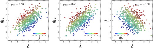
A toy model illustrating the relations between the relative BCG stellar mass |$\hat{m}_*$|, relative richness |$\hat{\lambda }$|, and relative concentration |$\hat{c}$| at fixed halo mass. The three panels show the distributions of 500 mock clusters generated with equation (29) on the planes of |$\hat{c}{-}\hat{m}_*$| (left), |$\hat{\lambda }{-}\hat{m}_*$| (middle), and |$\hat{c}{-}\hat{\lambda }$| (right), respectively. In each panel, each filled circle is colour-coded by the value of the third quantity (other than the quantities in the x- and y-axes) according to the inset colour bar. The Pearson cross-correlation coefficient is shown by the legend on the top left of each panel. Our toy model of equation (29) successfully reproduces the observed correlation between concentration and BCG stellar mass (left), BCG-satellite conformity (middle), and the simulation-predicted anticorrelation between concentration and richness (right).
7 SUMMARY AND CONCLUSION
We develop a prescription for the cluster assembly bias effect that ties the halo concentration measured by small-scale ΔΣ to the cluster bias measured by either ΔΣ or cluster–galaxy cross-correlation on large scales. By combining cluster conformity with assembly bias, we build an accurate model for the weak lensing profiles ΔΣ of the low- and high-|$M_*^{\texttt {BCG}}$| clusters across all distance scales. Our conformity + AB model of ΔΣ predicts that the high-|$M_*^{\texttt {BCG}}$| clusters have |${\sim }20{{\ \rm per\ cent}}$| more concentrated (c = 6.95) dark matter haloes but are |${\sim }10{{\ \rm per\ cent}}$| less biased (b = 2.85) than the low-|$M_*^{\texttt {BCG}}$| clusters (c = 5.87 and b = 3.11), in good agreement with the observations. Using the average membership distance as a proxy of the background contamination, we demonstrate that the impact of projection effects on the inferred conformity and assembly bias signal is likely small (Busch & White 2017; Zu et al. 2017; Sunayama et al. 2020).
We argue that a simple picture of the two-phase BCG–halo co-evolution can explain the complex connection between |$M_*^{\texttt {BCG}}$|, λ, and c at fixed halo mass, i.e. |$M_*^{\texttt {BCG}}$| is positively correlated with both c and λ despite the anticorrelation between c and λ. In this simple picture, the starbursting phase of the BCG in situ growth is induced by the rapid accretion and frequent mergers that built up the central core of the cluster haloes at high redshift, while the ex situ BCG stellar mass growth at late times is predominantly driven by the dry mergers with the massive satellites that sunk into the cluster centres via dynamical friction. Consequently, the in situ portion of |$M_*^{\texttt {BCG}}$| is tied to the halo concentration, while the ex situ portion of |$M_*^{\texttt {BCG}}$| naturally correlates with the richness of satellite galaxies. A simple toy model based on this physical picture can qualitatively reproduce the salient features of the observed |$M_*^{\texttt {BCG}}$|-c-λ connection.
The strength of the inferred conformity signal may depend on the cluster finder, especially the centroiding algorithm and the definition of richness. We plan to extend our analysis to other publicly available cluster catalogues, e.g. the Yang et al. (2021) halo-based group catalogue from DECaLS imaging (see also Tinker 2020; Zou et al. 2021) and the Wen & Han (2021) cluster catalogue based on HSC and WISE. Furthermore, the conformity signal could also depend on cosmology. Murata et al. (2019) showed that while the constraints on the mean richness-halo mass relation are consistent between the Planck and WMAP models, the best-fitting scatter for Planck is progressively larger than the WMAP model for lower-mass haloes. However, the conformity signal is primarily constrained by the dependence of average halo mass on |$M_*^{\texttt {BCG}}$| at fixed richness and therefore should be less affected by the size of the scatter in the richness-halo mass relation.
With the ever-increasing precision of cluster weak lensing measurements (Mandelbaum 2018), we will be able to routinely measure not only the average halo mass of clusters but also the average halo concentration robustly from the shape of ΔΣ on small scales, after marginalizing over the mis-centring (Zhang et al. 2019) and baryonic effects (Cromer et al. 2021). Meanwhile, the diminishing statistical uncertainties of cluster surveys demand a thorough physical understanding of the galaxy–halo connection at the high-mass end, which would greatly mitigate the systematic uncertainties in cluster cosmology (Wu et al. 2019, 2021) via the making of more realistic synthetic clusters (Varga et al. 2021). More important, an observationally motivated yet physically comprehensive model of galaxy–halo connection, e.g. an extension to our toy model of the |$M_*^{\texttt {BCG}}$|-c-λ connection in Section 6.3, could point us to a minimum-scatter proxy of halo mass (Bradshaw et al. 2020; Farahi, Ho & Trac 2020; Palmese et al. 2020; Tinker et al. 2021). Therefore, it is imperative that we incorporate the strong conformity and assembly bias effect into the modelling of galaxy–halo connection and weak lensing of clusters for next-generation cluster surveys, including the Rubin Observatory Legacy Survey of Space and Time (LSST; Ivezić et al. 2019), Euclid (Laureijs et al. 2011), Chinese Survey Space Telescope (CSST; Gong et al. 2019), and the Roman Space Telescope (Roman; Spergel et al. 2015).
ACKNOWLEDGEMENTS
We thank the anonymous referee for the helpful suggestions that have greatly improved this manuscript. We thank Weiguang Cui, Melanie Simet, and Rachel Mandelbaum for helpful discussions. We gracefully thank Christopher Conselice for suggesting the term ‘cluster conformity’ for describing the correlation between BCG and satellites. YZ acknowledges the support by the National Key Basic Research and Development Program of China (no. 2018YFA0404504), National Science Foundation of China (11873038, 11621303, 11890692, 12173024), the science research grants from the China Manned Space Project (no. CMS-CSST-2021-A01, CMS-CSST-2021-A02, CMS-CSST-2021-B01), the National One-Thousand Youth Talent Program of China, and the SJTU start-up fund (no. WF220407220). YZ and YPJ acknowledge the support by the 111 Project of the Ministry of Education under grant no. B20019. YZ thanks the wonderful hospitality by Cathy Huang during his visit at the Zhangjiang Hi-Tech Park during the summer of 2021.
DATA AVAILABILITY
The data underlying this article will be shared on reasonable request to the corresponding author.
Footnotes
We deliberately avoid the more commonly used nomenclature of ‘brightest cluster galaxies’ as BCGs, because we are interested in the properties of the central galaxies, which are not necessarily the brightest members in their host clusters (Chen et al. 2021).
REFERENCES
APPENDIX A: A PRESCRIPTION FOR CLUSTER ASSEMBLY BIAS
To calibrate an accurate prescription of cluster assembly bias, we employ a large-volume high-resolution cosmological N-body simulation from the CosmicGrowth suite developed by Jing (2019). In particular, we utilize the z = 0.23 (closest to the mean redshift of our cluster sample) snapshot of the Planck_2048_1200 simulation, which has a box length of |$1.2\, \mathrm{G}\mathrm{ pc/h}$| and a mass resolution of 1.76 × 10¹⁰h−1M⊙ at Planck cosmology. We refer readers to Jing (2019) for technical details of the simulation. We identify dark matter haloes using the spherical overdensity-based rockstar (Behroozi, Wechsler & Conroy 2013) halo finder and compute halo concentrations using the maximum circular velocity-based approach (Klypin, Trujillo-Gomez & Primack 2011; Prada et al. 2012).
We select all the haloes with mass between 1013 and 1015h−1M⊙ and divide them into six bins in halo mass. Within each halo mass bin, we measure the median |$\bar{c}$| and scatter σc of the concentration distribution and select the haloes within ±2σc into four concentration bins with equal 1 − σc widths. We then measure the three-dimensional (3D) isotropic halo–matter cross-correlation functions ξhm by cross-correlating the positions of haloes with that of dark matter particles, as shown in Fig. A1. The six panels of Fig. A1 present the ξhm measurements for the six halo mass bins of |$\lg M_\mathrm{ h}{=}13{-}13.29$|, 13.29−13.57, 13.57−13.86, 13.86−14.14, 14.14−14.43, and 14.43−15, respectively. In each panel, the main sub-panel shows the ξhm of haloes in four concentration bins: [ − 2σc, σc] (red), [ − σc, 0] (orange), [0, σc] (cyan), and [σc, 2σc] (purple), as well as the measurement for all the haloes in that mass bin (grey with error bars). The division of concentration bins is indicated by the concentration distribution in the inset panel, with each coloured segment mapped to one of the four concentration bins. We plot r2ξhm instead of ξhm in the y-axis to highlight the differences between the four concentration bins on both the small and large scales. The bottom sub-panel shows the ratio between the ξhm profile of each concentration bin and that of the all the haloes in that mass bin. We compute the uncertainties of ξhm and their ratios with Jackknife re-sampling, though we do not show the error bars (except for the grey curves) in Fig. A1 to avoid clutter.
![Dependence of the 3D isotropic halo–matter cross-correlation function ξhm on concentration in six halo mass bins ranging from 1013h−1M⊙ to 1015h−1M⊙ (increasing from left to right and from top to bottom). For each mass bin, the main sub-panel compares the ξhm of haloes in four concentration bins: [ − 2σc, σc] (red), [ − σc, 0] (orange), [0, σc] (cyan), and [σc, 2σc] (purple), illustrated by the four segments of concentration distribution in the inset panel. We plot r2ξhm instead of ξhm in the y-axes to highlight the difference between the four concentration bins on all distance scales. Grey curve with error bars indicates the ξhm of all the haloes in that mass bin. The bottom sub-panel shows the ratio profiles between the ξhm of four concentration bins and that of all haloes in the same mass bin. We calculate halo biases from the ξhm measurements on scales between 10h−1Mpc and 30h−1Mpc, where the biases are roughly linear.](https://oup.silverchair-cdn.com/oup/backfile/Content_public/Journal/mnras/511/2/10.1093_mnras_stac125/1/m_stac125figa1.jpeg?Expires=1750478244&Signature=gEEu5EgPqhtUdcFrZ6K02jcbnz0OGb0hsOLXhq3lKxdxdr~AsnIDcwGqjAeRr6ul4WH7LJbLvfrCTdCad5hgsy-gX-DvPASJyj8ctIvhE3GltHVJO8rjPquarD2eGMcOPMP3GiLmAsuKj7HtNDzYvAY6g-61YnVANjfDMJKwSHYEYW7eHYVxVSMS9ergJERaPpMoTy4ZHr081qT1~JVpmgYIXb76C7JJ-7rAYCIUNZE7JAMBUhgGQojeOjG2-3gf78k9ckuMlI2YE6uL1B4J95ESeGp9Y46MibOxMSvYYnSseGWwYc8Mg0y4yaDn3aVsQLxtp3L7CwWU~qa8SI62jQ__&Key-Pair-Id=APKAIE5G5CRDK6RD3PGA)
Dependence of the 3D isotropic halo–matter cross-correlation function ξhm on concentration in six halo mass bins ranging from 1013h−1M⊙ to 1015h−1M⊙ (increasing from left to right and from top to bottom). For each mass bin, the main sub-panel compares the ξhm of haloes in four concentration bins: [ − 2σc, σc] (red), [ − σc, 0] (orange), [0, σc] (cyan), and [σc, 2σc] (purple), illustrated by the four segments of concentration distribution in the inset panel. We plot r2ξhm instead of ξhm in the y-axes to highlight the difference between the four concentration bins on all distance scales. Grey curve with error bars indicates the ξhm of all the haloes in that mass bin. The bottom sub-panel shows the ratio profiles between the ξhm of four concentration bins and that of all haloes in the same mass bin. We calculate halo biases from the ξhm measurements on scales between 10h−1Mpc and 30h−1Mpc, where the biases are roughly linear.
The dependence of ξhm on halo concentration is consistent across all mass bins, with the low-concentration haloes showing stronger biases than the high-concentration systems. The probability distributions of concentration are reasonbaly Gaussian, with some level of skewness and kurtosis developed for the higher-mass bins. The lowest mass bin, however, does show a narrower range of variation of bias with concentration, as the concentration–bias relation would reverse its sign below the characteristic non-linear mass scale, i.e. low-concentration haloes would be less biased in the low halo mass regime (Gao et al. 2005). There, we drop the lowest mass bin of Fig. A1 from our assembly bias calibration. To accurately calibrate assembly bias well into the characteristic non-linear mass scale, a suite of extremely high-resolution simulations that can resolve haloes down to 1011h−1M⊙ is required, hence beyond the scope of this paper. None the less, since the main bulk of the halo mass distribution of our cluster sample is above |$\lg M_\mathrm{ h}{=}13.29$| (see Fig. 5), the systematic uncertainty of our assembly bias model caused by the omission of low-mass haloes should be small compared to the observational errors.
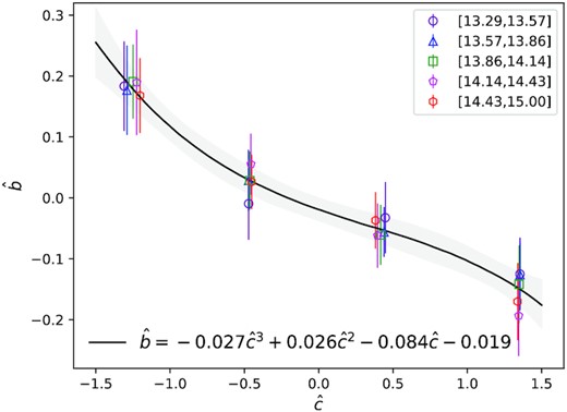
Our prescription of the cluster assembly bias calibrated for haloes at z ≃ 0.23. Symbols of different colours with error bars indicate the measurements of the relative bias |$\hat{b}$| (equation A2) as a function of the relative concentration |$\hat{c}$| (equation A1) in five different halo mass bins indicated by the legend in the top right. Black solid line is our third-order polynomial fit to the data points, with the best-fitting parameters indicated in the bottom left.
APPENDIX B: A JOINT MODEL OF CONFORMITY AND ASSEMBLY BIAS FOR |$\boldsymbol {\Delta \Sigma }$|
We are now ready to construct a comprehensive model of the cluster weak lensing profile ΔΣ by incorporating both the BCG-satellite conformity constrained in Section 4.3 and the cluster assembly bias calibrated in Fig. A2. In particular, in Section 5 we demonstrate the efficacy of our ΔΣ models by comparing their predicted full weak lensing profiles of the low- and high-|$M_*^{\texttt {BCG}}$| subsamples to the measurements from Paper I. We predict ΔΣ for the two cluster subsamples in two separate steps, with cluster assembly bias modelled in the first step and the BCG-satellite conformity modelled in the second. We describe each step in turn below.
To obtain a good description of the measured cluster weak lensing profiles on small scales, we adjust the values of |$\left\langle \hat{c}_\pm \right\rangle$| so that the average concentration of each subsample is consistent with the best-fitting average halo concentrations derived in Paper I, i.e. 〈c−〉 = 5.87 for the low-|$M_*^{\texttt {BCG}}$| and 〈c+〉 = 6.95 for the high-|$M_*^{\texttt {BCG}}$| subsamples, respectively. Assuming the mean concentration–mass relation from Zhao et al. (2009) and a constant concentration scatter of σc = 0.15, our best-fitting values are |$\left\langle \hat{c}_- \right\rangle {=}0.156$| and |$\left\langle \hat{c}_+ \right\rangle {=}1.045$| within the posterior mean conformity model, while in the anticonformity model they become |$\left\langle \hat{c}_- \right\rangle {=}0.17$| and |$\left\langle \hat{c}_+ \right\rangle {=}1.206$|. By applying those values of 〈c±〉, we can further infer the bias values via the cluster assembly bias prescription of equation (A3). In particular, within the conformity model, the biases are 〈b+〉 = 3.20 and 〈b−〉 = 3.21 when cluster assembly bias is switched off, and 〈b+〉 = 2.85 and 〈b−〉 = 3.11 when cluster assembly bias is on, respectively. We also infer 〈b+〉 = 3.78 and 〈b−〉 = 2.79 for the anticonformity but without applying cluster assembly bias, because the model is already ruled out regardless of the existence of cluster assembly bias. We adopt those best-fitting values of |$\left\langle \hat{c}_{\pm } \right\rangle$| and 〈b±〉 and predict the ΔΣ profiles for the low- and high-|$M_*^{\texttt {BCG}}$| subsamples under different assumptions of conformity and assembly bias.
