


ABSTRACT
A large fraction of stars are formed in dense clusters. In the cluster, close encounters between stars at distances less than 100 au are common. It has been shown that during close encounters planets can transfer between stars. Such captured planets will be on different orbits compared to planets formed in the system, often on very wide, eccentric, and inclined orbits. We examine how these captured planets affect Kuiper belt-like planetesimal belts in their new systems by examining the effects on habitable planets in systems containing an outer gas giant. We show that these captured planets can destabilize the belt, and we show that the fraction of the planetesimals that make it past the giant planets into the system to impact the habitable planet is independent of the captured planet’s orbital plane, whereas the fraction of the planetesimals that are removed and the rate at which they are removed depend strongly on the captured planet’s pericentre and inclination. We then examine a wide range of outcomes of planet capture and find that when a Jupiter-mass planet is captured it will in 40 per cent of cases destabilize the giant planets in the system and in 40 per cent of cases deplete the belt in a few Myr, i.e. not posing much risk to life on terrestrial planets that would be expected to develop later. In the final 20 per cent of cases, the result will be a flux of impactors 10–20 times greater than that on Earth that can persist for several Gyr, detrimental to the development of life on the planet.
1 INTRODUCTION
The majority of stars form in clusters (Lada & Lada 2003). These clusters have stellar densities of 100–1000 pc−3 (Dias et al. 2002; Lamers et al. 2005), compared to ∼1 pc−3 in the field (see e.g. Gaia Collaboration 2018), and lifetimes of several tens to hundreds of Myr (Gieles, Lamers & Portegies Zwart 2007). In such dense clusters, 10–20 per cent of solar-like stars will experience an encounter within 100 au with another star, which is close enough to affect the stability of existing planets (Malmberg, Davies & Heggie 2011).
Given that the giant planets form before gas dispersal in protoplanetary discs, typically within a few Myr after star formation (Machida et al. 2010; Piso & Youdin 2014; Piso, Youdin & Murray-Clay 2015; Bitsch et al. 2019), for most of these encounters the stars will have finished forming their giant planets. During these encounters, planets can be transferred between stars (Kenyon & Bromley 2004; Morbidelli, Emel’yanenko & Levison 2004; Jílková et al. 2015, 2016; Li, Mustill & Davies 2019). This can result in planets on orbits that are inconsistent with planet formation models. This is a possible explanation for the hypothesized presence of Planet 9 (Batygin & Brown 2016) on its (albeit loosely constrained; Brown & Batygin 2016) few hundred au wide orbit (Mustill, Raymond & Davies 2016).
In this paper, we will examine how capturing a planet will affect planets in the habitable zone. In particular, we consider systems like our own, i.e. a terrestrial planet at ∼1 au, with giant planets beyond it surrounded by a Kuiper belt-like disc of planetesimals (throughout the paper, we refer to this belt simply as ‘the belt’ and its component bodies as ‘planetesimal’). There are four ways in which the captured planet can affect them:
The planet can be captured on an orbit that crosses the orbits of planets in the system, meaning it can either directly scatter a planet in the habitable zone or trigger an instability among the outer planets. Instabilities among the outer planets can destabilize a large fraction of possible orbits in the habitable zone (Carrera, Davies & Johansen 2016; Kokaia, Davies & Mustill 2020).
The captured planet can induce Kozai oscillations on the existing planets, which can destabilize all of the planets without the captured planet ever having a close encounter with them. The stability of planetary systems with an external highly inclined companion has been well studied for both stellar and planetary companions by e.g. Innanen et al. (1997), Kaib, Raymond & Duncan (2011), Malmberg et al. (2011), Mustill, Davies & Johansen (2017), and Denham et al. (2019).
In the absence of an instability, the outer planets or a single outer planet can have its eccentricity pumped up putting it on an orbit crossing the habitable zone, which will destabilize most if not all possible orbits within it (Jones, Sleep & Chambers 2001; Menou & Tabachnik 2003; Matsumura, Ida & Nagasawa 2013; Agnew, Maddison & Horner 2018; Georgakarakos, Eggl & Dobbs-Dixon 2018).
Planetesimals in belts external to the planets such as the ones found in the Kuiper belt (which appear to be fairly common around Sun-like stars; Montesinos et al. 2016; Sibthorpe et al. 2018) can be directly scattered or undergo Kozai oscillations and end up crossing the orbits of the giant planets in the system. They can then be scattered further inwards and end up on orbits crossing the habitable zone. This can then lead to a large number of impacts on any planets in the habitable zone.
The main focus of the paper will be outcome (iv), with outcome (i) discussed briefly. In Section 2, we will discuss the theoretical framework of the Kozai mechanism and also show the results of an exploratory experiment comparing the theory with our simulation set-up. This set-up will be discussed in Section 3 and the findings from it will be presented in Section 4. In Section 5, we discuss the implications of said findings, perform some novel comparisons between our model and the Solar system, and then also explore the impact of having different set-ups.
2 THE KOZAI MECHANISM
The Kozai mechanism (Kozai 1962; Lidov 1962) is a secular three-body effect that can produce very large oscillations in eccentricity and inclination. Here follows a brief description of the process: Consider an inner body (A) and an outer companion (C) orbiting a central body (⋆). A particularly simple case of Kozai cycles occurs when the three conditions below are met (Innanen et al. 1997; Malmberg, Davies & Chambers 2007a).
aC ≫ aA: The semimajor axis of C needs to be much larger than the semimajor axis of A.
mC ≫ mA: The mass of C needs to be much larger than the mass of A.
180○ − icrit > i > icrit: The mutual inclination (i) between A and C needs to be between the critical angle icrit and 180○ − icrit, where |$i_{\rm crit}=\arcsin \sqrt{2/5}\approx 39.23^\circ$|.
When these conditions are met, the system will oscillate in eccentricity and in mutual inclination between i0 and icrit. Cycles in eccentricity and inclination will still happen if either of the first two conditions is not met. However, the formalism that follows will be less and less accurate as the mass and semimajor axis ratios approach unity (Katz, Dong & Malhotra 2011; Naoz et al. 2013a; Naoz, Yoshida & Gnedin 2013b; Antognini 2015).

2.1 Kozai between planets
The Kozai mechanism described in the previous section details how the system behaves in the test particle limit, i.e. when all the angular momentum is held by the inclined perturber.
The system that has been explored in greatest detail throughout this paper is set up as follows: a central body of one solar mass, an Earth-mass planet at 1 au, a Jupiter-mass planet on a circular orbit at 10 au, and an additional Jupiter-mass planet on a circular but inclined orbit at 100 au. We refer to each body as Sun, Earth, [lower case] jupiter, and Companion. The Companion being on a circular orbit is not realistic, but we chose to keep it so in order to do a straightforward comparison between the numerical and analytical results using the Kozai formalism.
We investigate how the behaviour of this system differs from what we expect from the analytical solution above by running a set of simulations for just these four bodies (SEjC) where we vary the inclination of the Companion (iC) from 0 to 1801 deg, with both the Earth and jupiter in the reference plane. In Fig. 2, we show the maximum eccentricity reached by jupiter during the 108 yr we run the simulation for as a function of Companion inclination. The black dashed line shows the theoretical expectation, which is symmetric about 90 deg as expected; given equation (5). The solid blue line that shows the simulated data is no longer symmetric due to the angular momentum of jupiter and the location of the maximum has now shifted from 90 to ∼100 deg. The flat peak of the blue line is due to the Sun having a radius of 0.2 au in the simulations, i.e. when anything gets within said distance it is removed. This was chosen for computational efficiency in the runs with planetesimals later on, but we chose to keep it as such here for consistency.
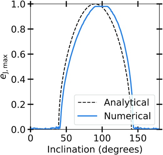
A range of simulations for the SEjC system. The dashed black line shows the theoretical emax predicted from equation (5), i.e. the test particle limit. The solid blue line shows the maximum eccentricity achieved by the jupiter in the SEjC runs.
This means that jupiter reaches an eccentricity of 0.98 for iC between 90 and 110 deg, rather than between 81 and 99 deg indicating an asymmetry between pro and retro-grade orbits. This makes sense because jupiter holds ∼1/3 of the system’s angular momentum and thus putting the Companion on a retrograde orbit will not invert the total angular momentum vector of the system.
2.2 Time-scales
As we will see later, time-scales will prove to be an important aspect of what happens when a planet is captured. This is because a planet on an orbit that is precessing sufficiently fast will not have its eccentricity pumped up by the Kozai mechanism (Kaib et al. 2011; Mustill et al. 2017; Denham et al. 2019). Orbits precess in any non-Keplerian potential (see e.g. Murray & Dermott 1999), i.e. any two bodies orbiting a central more massive body will precess.
3 SET-UP OF THE MAIN EXPERIMENTS
All the simulations were performed using the mercury N-body package (Chambers 1999). We used the Bulirsch–Stoer integrator with an accuracy parameter of 10−12 resulting in energy errors of <10−6. We set an ejection radius of 1000 au and set a stellar radius of 0.2 au. Both are done to speed up the simulations (reducing the number of bodies simulated and avoiding small pericentre passages). The stellar radius is also motivated physically as the planetesimals (test particles) simulated are icy bodies and would likely not survive such a pericentre passage.
3.1 The belt
To the SEjC system we now add planetesimals and examine how they interact with the Companion and with jupiter. For this, we use a belt analogous to the Kuiper belt using the prescription from Volk & Malhotra (2011).
We show this fraction (blue line) for aj = 10 au in Fig. 3 along with the fraction of planetesimals that can undergo Kozai cycles (black dashed line) for any given Companion inclination with respect to the reference frame.
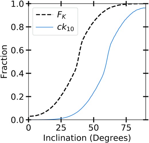
The black dashed line shows the fraction of test particles that can undergo Kozai cycles as a function of the inclination of the captured giant. Whereas the blue line shows the fraction of test particles that achieve a pericentre less than 10 au, i.e. the test particles that satisfy equation (11).
3.2 SEjC
We now go back to the SEjC system and simulate it with planetesimals. The planetary system contains one solar mass star, the Earth, jupiter, and a Companion. We set aj= 10 au, aC= 100 au, eC = 0, and mj = mC = MJ. This does also fulfill the inequality in equation (7), in fact any aC < 239 au with eC = 0 will do so for aj = 10 au. The inclinations simulated are iC = [25, 40, 55, 70, 85]○. We place Earth at 1 au and set it in the reference plane, whereas we give jupiter a small inclination (0–5 deg) and a small eccentricity (<0.01). This means that the mutual inclination between the Companion and Earth will exactly equal the Companion inclination in every realization (for each inclination we do a set of simulations with a small number of test particles), whereas the Earth–jupiter inclination will vary, mostly between 2–3 deg.
We do four different suites of runs, with three containing different subsets of planetesimal trajectories as determined in Fig. 3; the fourth being a retrograde version of the first:
full – Set where the planetesimal trajectories are simply drawn from the distributions described in the previous section – 100 realizations per inclination with 200 planetesimals each.
kozai – Set where only such planetesimals are drawn as to give Kozai oscillations, we do not do the 70 and 85 inclinations as Fig. 3 shows the fractions to be nearly identical to close kozai – 100 realizations with 200 planetesimals each.
close kozai – Set where only such planetesimals are drawn that give large enough Kozai oscillations to cross the orbit of jupiter – 300 realizations per inclination, 50 planetesimals in the first 150 runs, and 200 in the latter half of them.
full retro – Set where we reuse the initial conditions from the full simulations with only one thing changed, we set the companion on a ‘mirrored’ retrograde orbit. Given the broken symmetry we utilize Fig. 2 and define a mirrored system such that a system is mirrored if the companion on a retrograde orbit gives the same emax as its prograde equivalent. The mirrored inclinations are [25,40,55,70,85] → [161,146,136,125,–]. We do not do the 85 deg retrograde run as just as in the prograde run its mirror ends up pushing the planets into the star on a short time-scale, as seen in Fig. 2 – 100 realizations per inclination with 200 planetesimals each.
We will refer to SEjC runs as a1.n where a ∈ {f, k, ck} with f for full, k for kozai, and ck for close kozai, and n∈{1,5} denotes the five different inclinations. All of the simulations run for 108 yr.
4 RESULTS
Before even considering what happens with the planetesimals we consider jupiter as it too will undergo Kozai cycles, although it should be noted that the precession from a second giant planet in the system would have blocked the cycles. We can see in Fig. 2 that jupiter reaches high enough eccentricities (>0.9) to cross the orbit of the Earth for companion inclinations between 79 and 117 deg. This means that in 32.4 per cent of cases jupiter will reach sufficient eccentricities to cross the orbit of Earth leading to either a collision or a scattering which can either eject the Earth or send it into the Sun. We do indeed see this in the ck1.5 and f1.5 simulations but we report the behaviour of the planetesimals from those simulations regardless as most of the planetesimals will undergo several Kozai cycles and have time to reach their end state long before the 20–30 Myr it takes for the jupiter to increase its eccentricity and encounter the Earth.
4.1 SEjC – Earth impacts
The parameter values for the fits to the close encounters using equation (14) on the ck runs.
| Inclination | a | b |
|---|---|---|
| 25 | 0.22 ± 0.05 | 1.46 ± 0.03 |
| 40 | 0.40 ± 0.09 | 1.35 ± 0.04 |
| 55 | 0.32 ± 0.07 | 1.34 ± 0.04 |
| 70 | 0.12 ± 0.06 | 1.40 ± 0.04 |
| 85 | 0.19 ± 0.05 | 1.42 ± 0.04 |
| Inclination | a | b |
|---|---|---|
| 25 | 0.22 ± 0.05 | 1.46 ± 0.03 |
| 40 | 0.40 ± 0.09 | 1.35 ± 0.04 |
| 55 | 0.32 ± 0.07 | 1.34 ± 0.04 |
| 70 | 0.12 ± 0.06 | 1.40 ± 0.04 |
| 85 | 0.19 ± 0.05 | 1.42 ± 0.04 |
To compare the outcomes of the runs at the different inclinations we compare the ratio between the number of expected hits for an Earth-sized body with the number of planetesimals that get within 500 Earth radii. We plot these ratios for the different runs in Fig. 5. We see no clear trend with inclination and conclude that the outcomes at the different inclinations are consistent with each other.
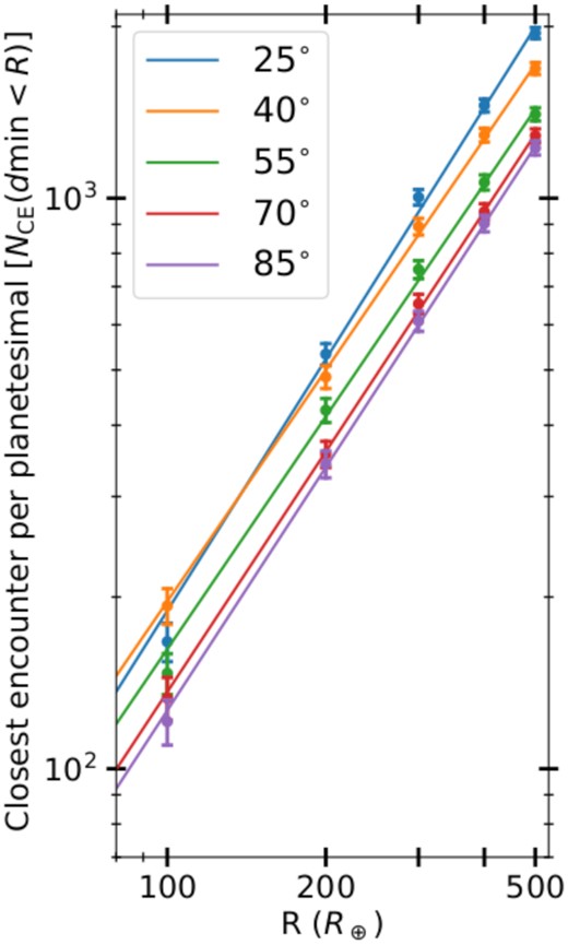
The number of planetesimals that have Earth–planetesimal close encounters where the closest approach is less than radius R for the five different inclinations.
This means that to get the fraction of planetesimals in the ck runs that would hit an Earth-sized planet we can stack the data from all the ck runs and compute the fraction. We find the fraction to be (7.1 ± 1.6) × 10−6. This fraction is interpreted as the fraction of planetesimals removed from the belt that end up hitting the Earth. The number of impacts this corresponds to depends on what fraction of the belt a given Companion destabilizes and the number of bodies in the belt. This is discussed in more detail in Section 5.
4.2 SEjC – planetesimals removal from belt
In Table 2, we show the outcome of the planetesimals in the k and f runs at two different times, 10 and 100 Myr. We pick 10 Myr because during this time the planetesimals undergo multiple cycles whereas jupiter does not have time to increase its eccentricity. If only the subset of planetesimals that are simulated in the ck runs end up crossing the orbit of jupiter we would expect the fractions crossing, fcross = ck10 for the full runs and fcross = ck10/FK for the k-runs. The table shows that after 10 Myr, the fraction of planetesimals removed is mostly consistent with the number of planetesimals that can cross the orbit of jupiter, whereas at later times significantly more of the planetesimals have been removed.
The outcomes of the kozai and full runs. fexpected is the fraction we expect to cross the orbit of J if only the ck subset were the ones crossing. fcross,10 and fcross,100 are the fractions of planetesimals that end up crossing the orbit of jupiter after 10 and 100 Myr. fremoved is the fraction of planetesimals removed after 100 Myr, either by being ejected or hitting the star or planets. Note: the output has a resolution in time of 10 kyr, i.e. if a particle crosses 10 au and is ejected within 10 kyr it will never be logged as having crossed the orbit of jupiter, resulting in an underestimation of fcross.
| System | fexpected | fcross,10 | fcross,100 | fremoved |
|---|---|---|---|---|
| k1.1 | 0.05 | 0.06 | 0.20 | 0.24 |
| k1.2 | 0.13 | 0.11 | 0.30 | 0.41 |
| k1.3 | 0.36 | 0.36 | 0.77 | 0.94 |
| f1.1 | 0.01 | 0.01 | 0.05 | 0.05 |
| f1.2 | 0.09 | 0.08 | 0.23 | 0.27 |
| f1.2r | 0.04 | 0.04 | 0.11 | 0.14 |
| f1.3 | 0.33 | 0.39 | 0.83 | 0.91 |
| f1.3r | 0.14 | 0.12 | 0.47 | 0.54 |
| f1.4 | 0.79 | 0.81 | 0.95 | 1.0 |
| f1.4r | 0.33 | 0.38 | 0.84 | 0.95 |
| f1.5 | 0.95 | 0.91 | 0.95 | 1.0 |
This means that there are two processes removing planetesimals from the system. The first and faster one is jupiter removing the planetesimals that have their eccentricity pumped up by the Companion. The second process is a combination of planetesimals being pushed to higher eccentricities through interactions with the Companion and jupiter eventually putting them on a jupiter-crossing orbit, which in some cases is due to jupiter itself gaining some eccentricity, leading to their eventual removal. Furthermore, planetesimals can be being removed directly by the Companion from the belt. The latter of these can happen because the Companion encounters the planetesimals at their apocentre giving encounters with very low ΔV during which the Companion can do enough work to unbind the planetesimals.
4.2.1 Examining longer time-scales
5 DISCUSSION
5.1 Initial impact rates
It is quite apparent from Table 2 that the Kozai formalism only works as a valid approximation for the first ∼10 Myr, i.e. that the number of jupiter-crossing planetesimals is well approximated by the ck-fraction as seen in Fig. 3. Given that we in Section 4.1 showed that 7.1 in 106 jupiter-crossing planetesimals will impact the Earth we can determine the impact rate during those first 10 Myr in the SEjC system. We consider the number of >1 km sized bodies in the primordial Kuiper Belt, which we from Nesvorný & Vokrouhlický (2016) find to be ∼1012. The impact rates are shown in Fig. 6, where we plot the cumulative density function of the average impact rate distribution for >1 km sized bodies using the Kuiper belt. The red line in the figure shows that roughly one third of captures will result in jupiter eventually ejecting the Earth, this, however, happens on a longer time-scale meaning that we can determine the impact rate before the orbits of the planets cross and for that reason we can include rates above the red line in the figure.
We consider the impact rate using the primordial Kuiper belt because capture of a planet is not possible after the star leaves its birth cluster. Therefore, these impacts would only occur very early in the evolution of the system. Taking the Solar system as a point of comparison, these high impact rates are comparable to the impact rates determined for the Late Heavy Bombardment (Zahnle et al. 2003), which occurred very early in the history of our system.
5.2 The companion as a transient perturber
Concerning our Solar system, using wide field infra-red data from WISE, Luhman (2014) excludes the possibility of having any planet above the mass of Saturn within |$28\, 000$| au and mass of Jupiter within |$82\, 000$| au, excluding the possibility of the Sun having a Companion such as the one we have simulated. However, as we have shown, many companions can deplete a large fraction of the Kuiper belt in only a few Myr. This means that most of the work could have been done while the Sun was still in its birth cluster. Therefore, even if the Companion is removed in a subsequent encounter a couple of Myr after capture it can already have removed a large fraction of the Kuiper Belt. In fact, Malmberg et al. (2007b) find that stars that have a close encounter in their birth cluster, have a higher probability of having another close encounter than they initially had to have one at all. Given that a captured Companion that affects the Kuiper belt but does not leave a significant dynamical imprint on the inner planets must be on quite a wide orbit, it can be unbound rather easily in subsequent close encounters in the birth cluster. If the Companion is not removed in the birth cluster it cannot later be removed by other stars as sufficiently close encounters only occur once every 1011 yr or so (Bailer-Jones et al. 2018), but it could have been removed by a giant molecular cloud. From Gustafsson et al. (2016), we see that the tidal field of a massive GMC (∼106 M⊙) could do enough work on the planet to unbind it as the star passes through the giant molecular cloud. Such encounters would occur approximately once per Gyr (Kokaia & Davies 2019).
5.3 Later impact rates
It is clear that using the Kozai mechanism to approximate impact rates at a later time does not work. In order to do this we consider the 1 Gyr simulations done in Section 4.2.1. As in the previous section, we determine the impact rates by using the number of bodies in the Kuiper belt and using equation (15). We find that 1 Gyr after the capture, for the three different inclinations and a 20 M⊕ Kuiper belt, we find impact rates of >1 km sized objects per Myr of: [108, 110, 8.5]. Here, we have assumed no other depletion of the Kuiper belt.
We can compare the rates we find with the inferred present-day impact rate on the Earth.3 While not very well constrained, the most recent estimates give a rate of ∼1 per Myr for asteroids with a radius of 1 km (Wheeler & Mathias 2019). This means that a capture on a low inclination will actually be worse for an Earth-like planet than a high one (assuming it is not so high as to destabilize it). This is because, rather than a short cataclysmic period during which most of the Kuiper belt is depleted before life has had any chance to develop, it instead results in an increased rate over a much longer time, giving life on the planet less time to recover and develop between potential extinction events.
5.3.1 Generalizing farther
We have hitherto been using a rather naive simulation set-up for our Companion in order to use the Kozai formalism; however, as we have shown, this does not work on longer time-scales. We now do a set of simulations where the Companion has a realistic eccentricity for a captured planet and consequently we also use larger semimajor axes and measure the depletion of the belt for these orbits. We chose semimajor axes and eccentricity such that three different depletion regimes for the belt (one additional regime exists if one considers planet stability separately) are probed:
The Companion can orbit-cross the belt disrupting it directly.
The Companion can pump up the eccentricities of the planetesimals with either the Companion itself or jupiter ejecting them later.
The Companion can pump up the eccentricities of the planetesimals and then have them be removed by only jupiter.
To explore the outcome of companions captured on their possible different orbits we do a suite of low resolution simulations. The chosen orbits are shown in Fig. 7 as black crosses with the different regimes highlighted, for each black cross we do low-resolution simulations (1000 planetesimals per run) at 6 different Companion inclinations; 40, 55, and 70 deg prograde and 124, 134, and 145 deg retrograde selected by looking at Fig. 2 as described in Section 3.
5.3.2 Mapping the outcome-space
For each run we log the mean impact rate and use this to map the outcome-space following Companion capture. We explore the outcome-space by drawing Companions with random eccentricities and inclinations at the two semimajor axes. The eccentricity is drawn from a thermal distribution and the inclination from an isotropic distribution (Li et al. 2019). For each of the |$40\, 000$| Companion inclination and eccentricity drawn, we interpolate between the results from the runs described above and determine the time during which the impact rate greater than the impact rate on present Earth and the mean impact rate during this time-period.
We stack all of the outcomes and do a kernel density estimate, shown in Fig. 8. The first thing to note is that the figure only shows approximately 60 per cent of the outcomes. At both semimajor axes nearly 40 per cent (∼30 per cent due to Companion inclination and ∼10 per cent due to capture on high eccentricity) of captured Companions lead to the system becoming unstable.
The remaining ∼60 per cent of the time one of two things tends to happen:
High enhancement over a short period of time: companions that cross the belt or get near it or have a high inclination but not so high as to destabilize the system.
Low enhancement over a long time: companions that have a moderate inclination and a pericentre greater than 90 or so au. These companions can deplete most if not all of the belt given sufficient time and it results in an enhancement by a factor of 10–20 on a time-scale of Gyr.
We see here that the type of Companions that we concluded pose the greatest danger for life on a habitable planet when discussing the initial 1 Gyr simulations corresponding to a considerable fraction of possible Companion orbits. That is, the low-inclination Companions (25 and 40 deg but for more distant pericentres also the 50 deg) as they can produce an enhancement that persists for a much longer time.
6 CONCLUSIONS
Using a simple model of a planetary system with a planet in its habitable zone, we have studied the impact that capturing a planet on a wide, inclined orbit would have on the habitability of the system by considering the delivery of impactors. From this simple model, we then generalized further and considered the possible outcomes of capturing planets in systems with primordial planetesimal discs comparable to what is inferred for the primordial trans-Neptunian disc of the Solar system. Our key findings are as follows:
We show that due to the planetary system not being in the test particle limit, the Kozai oscillations deviate somewhat from the analytical description of the problem (Innanen et al. 1997), as we can see in Fig. 2. Regardless, we use the theory to determine the fraction of planetesimals that cross the orbit of jupiter and show that this is a valid approximation for what happens in the first 10 Myr of the system, for all Companion inclinations, as shown in Table 2.
For the SEjC system (Sun + Earth + Jupiter-mass planet at 10 au + Jupiter-mass Companion at 100 au), we find that for all inclinations roughly 7 out of 106 planetesimals that are destabilized will hit the Earth (Figs 4 and 5).
The impact rates due to a Companion captured early in a systems life are comparable to the Late Heavy Bombardment.
Inclined captured companions are very effective at clearing out the belt, with Companions that have an inclination greater than 55 deg (∼60 per cent of an isotropic distribution) and pericentre less than 100 au eventually clearing out the whole belt. This is contingent on the precession from the inner planets on the belt being slower than the Kozai oscillations.
With e ∼ 0.7 for captured planets as it follows a thermal distribution (see e.g. Li et al. 2019), the pericentres will likely often be small and captured planets will often remove a large fraction of the belts.
For habitable planets, Companions captured on low-inclination orbits have worse consequences, as it can give an enhanced impact rate for several Gyr (Fig. 8), rather than the short cataclysmic event produced by highly inclined captured companion.
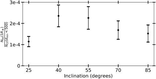
The number of planetesimals expected to hit an Earth-sized planet in our simulations divided by the number that get within 500 Earth radii of the Earth.
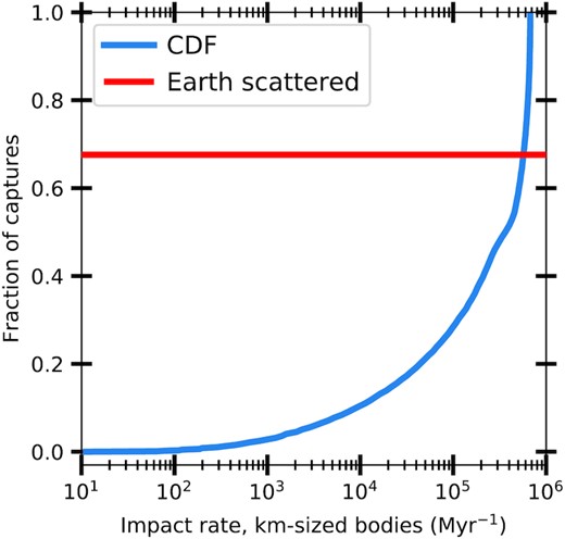
The blue line shows the CDF of the average number of impacts per Myr of bodies greater than 1 km as a function in the first 10 Myr following the capture of a planet on isotropically distributed orbit orientations. The numbers are calculated assuming a 20 M⊕ primordial Kuiper belt. The red line shows the limit above which the outcome is that the Earth ends up being either ejected or scattered and removed from the system.
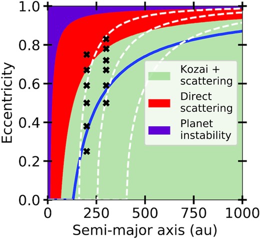
The different effects that are dominant for different a and e for captured planets. Planets captured in the purple region will disrupt the whole system. In the red region, they will be orbit-cross the belt and disrupt it. In the green region, planetesimals need to have their eccentricities increased through Kozai oscillations in order to be scattered by either the planets in the system or the companion, where the blue line is a line of constant pericenter and indicates the region within which the Companion can get within a Hill radius and scatter high-eccentricity (e ∼ 1) planetesimals. The black crosses show where we have done 1 Gyr long simulations with a Jupiter-mass companion and a Jupiter-mass internal planet at 5 au in order to determine what fraction is depleted. The white lines show where the precession from a Jupiter-mass inner planet with a semimajor axis of (from left to right) 2.5, 5, and 10 au blocks the Kozai cycles of the planetesimals.
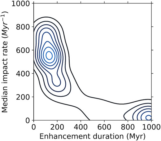
A kernel density estimate of the outcome space for the enhancement duration and corresponding mean enhancement for captured companions with semimajor axis of 200 and 300. The contours identify the highest density regions in the outcome space, based on the |$80\, 000$| randomly drawn Companions. The figure is generated by drawing eccentricities from a thermal distribution and inclinations from an isotropic distribution and then interpolating between the simulations done in Fig. 7.
ACKNOWLEDGEMENTS
The authors are supported by the project grant 2014.0017 ‘IMPACT’ from the Knut and Alice Wallenberg Foundation. AJM acknowledges support from the Swedish Research Council (starting grant 2017-04945) and from the Swedish National Space Agency (career grant 120/19C). The computations were enabled by resources provided by the Swedish National Infrastructure for Computing (SNIC) at LUNARC partially funded by the Swedish Research Council through grant agreement no. 2016-07213.
DATA AVAILABILITY
The data underlying this article will be shared on reasonable request to the corresponding author
Footnotes
Inclinations for the Companion above 90 deg denote retrograde orbits.
Note that Martin & Livio (2021) found that the collision cross-section does not scale as R2 and attributed this to gravitational focusing.
It should, however, be noted that the vast majority of Earth impactors originate in the asteroid belt and not the Kuiper belt (Strom et al. 2005).
