Out of one, many: distinguishing time delays from lensed supernovae Free

ABSTRACT

1 INTRODUCTION

Time delays in strong gravitational lens systems are one of the few dimensionful quantities that can be measured cosmologically. This enables an absolute distance measurement, rather than a ratio of distances, and so determines an absolute cosmic length-scale, e.g. the Hubble constant (Refsdal 1964). The time delay distance formed from the time delay involves combinations of distances from observer to source, observer to lens, and lens to source; this is a valuable probe of both the cosmic expansion behaviour and hence dark energy, and spatial curvature (Linder 2004, 2011; Treu & Marshall 2016; Liao et al. 2020; Millon et al. 2020; Shajib et al. 2020; Wong et al. 2020).

Each strongly lensed source is split so as to appear as multiple images, with generally the central lensed image unobservable due to lens galaxy obscuration, leaving two or four images. These images will be magnified in flux, and delayed in time, relative to the source flux and each other. Type Ia supernovae (hereafter just SN) have particular advantages as gravitationally lensed sources, as they are time variable (so time delays are detectable), their intrinsic time variation is fairly well known, the observations needed to measure time delays span a month or two rather than years as for lensed quasars, and the SN distances are standardizable, simplifying the lens system modelling.

If the multiple images can be resolved, i.e. their angular separations are greater than the observing resolution, then each image can be measured separately. Some particular recent work on such lensed supernova cosmology appears in, e.g. Huber et al. (2021), Pierel et al. (2021) and Rodney et al. (2021). However, for worse image resolution, smaller lensing masses, or less favourable geometry of the lens and source positions, the images may overlap and blend together – be unresolved. In this case, only a single combined light curve (flux versus time) can be measured, defining a system. We only use this observed light-curve data.

We focus here on such unresolved lensed SN, investigating whether we can determine from a combined light curve its constituent elements: is it lensed or unlensed, how many images, and what are their time delays (and magnifications, to a lesser extent). For unresolved lensed supernovae this work covers the key range of 6–14 d motivated by the expected distribution of time delays generally peaked around 10 d as in, e.g. Goldstein, Nugent & Goobar (2019). This extends Paper 1 (Bag et al. 2021) in this series by going beyond two-image systems to allow four images and a more robust exploration of multiplicity, and using a complementary fitting method, also without a fixed source template.

In Section 2, we describe the new fitting method and crosscheck it against both simulations and the previous method for two images. We analyse it for four-image systems in Section 3 and quantify its precision, accuracy, and range of robustness against simulations. Section 4 investigates determination of multiplicity, i.e. distinguishing unlensed (one-image) systems from two-image from four-image systems, presenting the ‘confusion matrix’ between them. We summarize the current state and future work in fitting unresolved lensed SN in Section 5.

2 FREEFORM FITTING

If one knew the source time evolution U(t) perfectly, then fitting for Δt_i, μ_i is straightforward. However, SN do vary in their light curve intrinsically, and any template adopted will lead to errors, and possibly biases, in the extracted time delays. Furthermore, we wish to keep our method reasonably general so it might be applicable in the future to other lensed transients besides Type Ia supernovae. Therefore, we did not adopt a fixed template in Paper 1, and do not here.

2.1 Free within bounds

In Paper 1, we took a base light-curve form with an asymmetric rise and fall (specifically a lognormal) and multiplied it with a Crossing hyper-function (fourth-order polynomial constructed from the first four Chebyshev polynomials) (Shafieloo, Clifton & Ferreira 2011; Shafieloo 2012a, b; Hazra & Shafieloo 2014). This gives considerable freedom for the light-curve shape. However, it does correlate the shape at one time with that at another time (recall the Chebyshev polynomials represent a linear tilt, parabolic curvature, etc. as they increase in order). Therefore, we also explored an alternate form allowing freedom in the light-curve shape, which we use in this paper.

The hyperparameters h_j are independently chosen at nodes t_k throughout the SN phase. The light curve in between nodes, i.e. the full U_j(t), is formed by multiplying a Gaussian kernel smoothing in time of the 1 + h_j(t_k) factor (denoted by the subscript GS(t); the smoothing length is itself a hyperparameter, lying in [3, 8] d) by a linear spline of H_j (the Hsiao template is defined at discrete epochs). We found this works better and is more computationally efficient than Gaussian smoothing (or splining) both factors. The number of nodes used is typically 50–70, depending on the observation range. Too small a number of nodes will not give sufficient freedom for variations, while too large a number of nodes will oversample the data as well as increase the computational cost. We experimented with both adaptive and equal time spacing, and found equal spacing to work well, avoiding the potential for adaptive spacing to become too sparse in certain epochs and miss useful features (e.g. troughs as well as peaks inform the time delay estimation).

As in Paper 1, we simulate data using our lcsimulator code based on the sncosmo (Barbary et al. 2020) python package, with light curves generated by applying noise and observing characteristics as in (Goldstein et al. 2019) to Hsiao spectra (see Appendix  A for tests with alternative light curves). The modelled light curves in g, r, i ZTF bands include observations with ∼2−4 d cadences with the flux uncertainties set to 5 per cent of the peak value. We normalize the input data to unit intervals in flux and time for consistent treatment of numerical precision. For a system modelled with N_image images, then the N_image − 1 relative time delays and N_image − 1 relative magnifications are derived from N_image absolute time positions and N_image magnifications.

We infer the time delays and relative magnifications using the No-U-Turn Hamiltonian Monte Carlo (HMC) sampler within CmdStan, the command-line interface to the Stan statistical modelling language (Stan Development Team 2021). Our typical HMC run includes eight chains, each with 1400 iterations and 250 warm up steps, with a system taking ∼0.4–4 h per chain, depending on the number of parameters (images) fit.

2.2 Comparison with crossing method

Advantages exist for each one of the fitting methods we apply to lensed light curves. The method of Paper 1, which we call the crossing method, allows the amplitude of deviation from the base form to vary widely, but places some constraints on the shape deviations. The freeform method here allows the shape of the light curve to vary widely but bounds the amplitudes of deviation. Allowing both shape and amplitude to vary without constraint is untenable as strong degeneracies are introduced such that, for example, an unlensed SN could be made to look like a blend of two images. We believe both the freeform and crossing method are useful, and provide valuable crosschecks.

We begin the comparison between the two by considering the two-image systems used in Paper 1 for blind testing. By fitting them with the freeform technique, we can directly compare the results.

Fig. 1 shows the results for this paper’s freeform technique (left) and Paper 1’s crossing technique (right) for those 100 systems. The top panels show Δt_fit versus Δt_true, the middle panels show the cumulative distribution function plots, and the lower panels the Δt_fit − Δt_true histograms.

Figure 1.

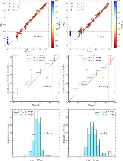
Blind tests using the freeform method (left-hand panels) and crossing technique (right-hand panels) on a set of 100 systems, with 9 unlensed and 91 two-image systems with time delays are distributed over 6−30 d. (Top panels) Time delay fits lie closely along the diagonal Δt_fit = Δt_true. For Δt_fit < 10 d, the crossing technique of Paper 1 tends to level out, while the freeform method continues to follow the diagonal. Unlensed systems (Δt_true = 0) are also clearly distinct from Δt_fit ≥ 10 fits with the freeform method. Error bars show the 95 per cent confidence intervals. (Middle panels) The cumulative distribution functions are shown for the systems with Δt_fit ≥ 10 d (blue) and Δt_fit ≥ 15 d (orange). The central 68 per cent of fit probability encompasses 65–68 per cent probability in the freeform case, showing excellent accuracy, an improvement over the 52–56 per cent of the crossing technique. (Bottom panels) Histograms of the time delay fits versus truth. Both show good peakiness around the truth.

Open in new tabDownload slide

For Δt_fit versus Δt_true, both techniques do quite well for Δt_fit ≥ 10 d, tightly following the diagonal, i.e. truth. The freeform method continues to follow the diagonal below 10 d, down to about 6 d (this was the limit of the Paper 1 testing; in Appendix  B here we see it actually works well to 2 d), while the crossing technique had levelled off with Δt_fit = 10 (all Δt are given in units of days). Also, for the unlensed systems (Δt_true = 0), the freeform method seems to control the fit somewhat better, keeping false positives well below Δt_fit = 10, unlike the crossing technique. This makes the freeform method appear promising for application to the four-image fits of the next section.

For the cumulative distribution functions (CDFs), the key characteristic is whether the distribution has slope one, i.e. the fit distribution follows the true distribution, in the central part of the diagram, indicating reliable fit uncertainties. We indicate the central 68 per cent probability distribution, between the 0.16 and 0.84 quantiles, by the vertical dotted lines. In that central 68 per cent probability, the freeform method fits occur 65–68 per cent of the time (depending on the cut-off in Δt_fit), demonstrating its accuracy, while the crossing technique had 52–56 per cent. Note that the vertical offset from the diagonal is due to a sample selection bias due to the imposed cut-off in Δt_fit, so that quantile zero is shifted to CDF >0; but again, the central part of the diagram is the most important.

The histograms of Δt_fit − Δt_true in Fig. 1 for Δt_fit ≥ 10 d show that the freeform approach accurately recovers the true time delays, with better than 1.25 d precision in ∼97 per cent of the cases, with accuracy ≲0.1 d. The freeform nature of the approach allows greater flexibility in the light-curve shape for robustness and eliminates the bias seen for the crossing method when 10 ≤ Δt_fit < 15.

Thus, the freeform technique has shown good accuracy and precision on two-image systems, motivating its use for four-image systems as well. We note that both approaches have advantages in particular areas. The crossing technique from Paper 1 starts from a form that is merely a rise and fall of flux, i.e. a fairly generic transient, without assuming it comes from an SN Ia, while the freeform technique does use deviations around a Hsiao SN Ia light curve. We might expect the crossing technique to be useful for unclassified transients, and then the freeform method to be more accurate for those suspected of being SN Ia. In the remainder of the paper we assume we are dealing with potentially lensed (one, two, or four images) SN Ia and employ the freeform method.

3 TIME DELAYS OF FOUR IMAGES

Having established that the freeform method works well on two-image systems, and distinguishes them from unlensed SN, we now proceed further and consider four-image systems (recall that strong lensing generally produces two or four visible images, not an odd number).

For four-image systems, there are four (unobservable) times t₁, t₂, t₃, t₄ associated with the four images, and three observable, independent relative time delays, Δt_AB, Δt_BC, Δt_CD. We use the numerical 1–4 and alphabetical A−D notation to emphasize the difference between unobservables and observables. Furthermore, there are four magnifications relative to the unlensed source flux, so there are a large number of permutations for the test system parameters. We therefore carry out two types of studies, one with systematic time delays and one with random time delays within a range.

First, we systematically study the accuracy of four-image fits by considering equal true delays: Δt_AB = Δt_BC = Δt_CD ≡ ΔT for ΔT = 4, 6, 8, 10, 12 d. We still fit for each time delay as independent free parameters. These systems are simulated with a flux noise level of 5 per cent of peak flux and a variety of image magnifications.

Fig. 2 shows the fits, relative to truth, for the three relative time delays Δt_AB, Δt_BC, Δt_CD for each of 10 four-image systems (we choose 10 systems randomly, enough to be statistically informative while not swamping the figure with 100 + data bars). We exhibit the cases for ΔT = 6 (left-hand panel) and ΔT = 10 (middle panel). While the fits have more variation than those for two images, nearly all contain the true value within the 95 per cent uncertainties. Even for ΔT = 6 (well below what we will use), there is clear recognition that it is lensed at some non-zero time delay.

Figure 2.

The time delay deviations from the truth in four-image systems for the equal time delay differences ΔT = 6 (left-hand panel), ΔT = 10 (middle panel), and randomly chosen from the Δt_i = [10, 14] interval (right-hand panel). The thin dashed and dotted vertical lines are used to indicate 2 and 3 d deviations, respectively. Error bars show the 95 per cent confidence intervals.

Open in new tabDownload slide

While we can fit four images well, plus distinguish them from the unlensed (zero time delay) case, we also want to see if we can distinguish them from the two image, lensed case. We therefore take the same systems and fit them as two-image systems as well, i.e. with a single relative time delay and a relative magnification.

Fig. 3 evaluates the relative χ² of the fit with four images relative to the fit with two images, as a function of true (four images) time delay spacing ΔT. If |$\Delta \chi ^2\equiv \chi ^2_{\rm min,4im}-\chi ^2_{\rm min,2im}\lt 0$|⁠, this means the four-image fit is preferred. However, as the four-image fit has four more parameters (two more time delays and two more relative magnifications), one might also look at the Akaike Information Criterion AIC =Δχ² − 2ΔN_dof. Then four images is robustly preferred when Δχ² < −8. These two criteria are shown as the dotted red and dashed magenta horizontal lines, respectively. We see that for ΔT > 8 d we can have significant confidence that we can distinguish four image from two-image lensed systems.

Figure 3.

Distinction between systems with four images and with two images is statistically highly significant for time delay spacing of greater than 8 d, generated for four-image systems. Error bars give the mean Δχ² difference and 68 per cent confidence region at each ΔT spacing. Fits with Δχ² < 0 (dotted red line) correctly prefer a four-image fit, while those with Δχ² < −8 (dashed magenta line) have Akaike Information Criterion AIC <0, accounting for the four extra parameters of a four- versus two-image fit, and hence are fully robust.

Open in new tabDownload slide

For the second study, we focus on time delays randomly distributed in the range Δt_i = [10, 14], where the subscript runs over AB, BC, CD. While we have seen that we can fit well smaller time delays for four-image systems, and for two-image systems, we will not have as robust confidence that we can tell the two cases apart. Therefore, we concentrate on this range, which should be the most challenging of the fits for which we have confidence not only in the fits themselves but the number of images as well (see Section 4 for further investigation). We also randomly select the magnifications μ_i.

For the magnification we impose μ_i > 0.25, since recall that μ_i = 0 means there is no image (so a four-image system with two μ_i = 0 is really a two-image system) and there is a perfect degeneracy for all values of that Δt_i, while for μ_i near zero such a low-amplitude bump is degenerate with a local shape perturbation h(t). Thus the condition μ_i > 0.25 is employed to avoid these issues and enable robust fit convergence. The upper bound is μ_i < 4.

The right-hand panel of Fig. 2 illustrates some time delay fits relative to the truth for these varying delay systems. The best fits are scattered about the truth, with no strong correlation between different time delays in a system, i.e. if one is on the positive side, the others may be on the positive or negative side. (More quantitatively, the correlation coefficients are ≲0.5.) As for the previous study of equal time delays, the fits are well consistent with the truth. Fig. 4 shows two examples of the four-image fit to the observed light-curve data, one with equal ΔT = 12 and one with time delays in the range Δt_i = [10, 14]. The points with error bars are the observed data, with the thick solid line being the light curve constructed by the sum of the four-image fits. The thin solid curves are the true image fluxes and the non-solid curves the fit reconstructions – remember, the only observable is the data points of the unresolved, summed light curve. The fit looks quite good, with excellent χ² and accurate time delay fits. The magnification fits are less good but not unreasonable. Our main focus however is identifying that an unresolved system is in fact a lensed system – out of one, many – and how many images, rather than optimizing per se the time delay and magnification estimation.

Figure 4.

The simulated four-image data with |$5{{\ \rm per\ cent}}$| noise level are shown for two systems, with equidistant ΔT = 12 time delays (left-hand column) and randomly distributed time delays in the range Δt_i = [10, 14] (right-hand column). The upper, middle, and bottom rows show the light curves in g, r, i bands, respectively. The thin solid black and blue pairs of lines are the true light curves of individual images. The dashed, dotted, dash–dotted, and dash–double-dotted lines are the individual image flux reconstructions of our model using the best-fitting parameters. The extracted time delays and magnification ratios as well as their true counterparts are indicated in each panel. The χ² values in the boxed texts indicate how well the reconstructed light curves fit the observations in comparison to the true ones.

Open in new tabDownload slide

4 HOW MANY IMAGES?

While obtaining four good image fits for data simulated with four images (or two for two) is important and valuable, we will not know the true number of images behind observed data (unlike for resolved lensed systems). Therefore, it is essential that we be able to distinguish systems with one (unlensed) versus two versus four images. Fitting a system with the incorrect number of images will likely lead to either degeneracies or biases.

We have already explored this partially with Fig. 3, and found robust distinction between four images and two images for ΔT ≳ 8 d. Now we examine this more thoroughly, forming a statistical confusion matrix between one- (unlensed), two-, and four-image systems, for realizations of random time delays Δt_i = [10, 14] and magnifications.

We simulate one-, two-, and four-image systems, 100 of each, and fit every one with one, two, and four images (e.g. not just true two with fit two, but true two with fit one, two, and four). By examining the Δχ² minima, and AIC, between the N and M image fits, we can decide whether we can robustly identify the number of images, and determine the time delays for the optimized case. The results of the fitting to simulations is summarized in the confusion matrix, with entries for each case where there are N images simulated, i.e. truth, and M images fit, for N, M = 1, 2, 4. We assign the system to the highest number of images for which the AIC <0 and the fit time delays of the images exceed a given threshold, e.g. Δt_fit ≥ 10 d. The fraction of true systems in each image category fit is given in the matrix entries.

Table 1 shows the results for our fiducial threshold, Δt_fit ≥ 10 d. The confusion matrix is perfectly diagonal, showing purity of classification. As we have already seen in the previous sections, the time delay fit accuracy is excellent as well.

Table 1.

Open in new tab

The confusion matrix showing the performance of our one-, two-, four-image models on a simulation set consisting of 100 unlensed systems, 100 two-image and 100 two-image lensed systems. The lensed systems have true adjacent time delays random in [10, 14] and magnification ratios in [0.5, 1.5]. The threshold is Δt_fit ≥ 10 d.

Table 1.

Open in new tab

The confusion matrix showing the performance of our one-, two-, four-image models on a simulation set consisting of 100 unlensed systems, 100 two-image and 100 two-image lensed systems. The lensed systems have true adjacent time delays random in [10, 14] and magnification ratios in [0.5, 1.5]. The threshold is Δt_fit ≥ 10 d.

Studying the results as we reduce the threshold below our fiducial, we see in Table 2 that we still identify the number of images in the system perfectly for a threshold of Δt_fit ≥ 8 d. Note we do have 10 per cent of two-image systems that are fit as four-image systems with one time delay greater than 8 d, but 0 per cent with two time delays greater than 8 d, and hence would not identify this as a four-image system above threshold. It is not until the threshold is lowered to Δt_fit ≥ 6 d that the confusion matrix becomes offdiagonal, as seen in Table 3.

Table 2.

Open in new tab

As Table 1 but with a threshold of Δt_fit ≥ 8 d.

Table 2.

Open in new tab

As Table 1 but with a threshold of Δt_fit ≥ 8 d.

Table 3.

Open in new tab

As Table 1 but with a threshold of Δt_fit ≥ 6 d.

Table 3.

Open in new tab

As Table 1 but with a threshold of Δt_fit ≥ 6 d.

Thus, the freeform method can successfully identify both the number of unresolved images, and the individual image time delays, for Δt_fit ≳ 10 d.

5 CONCLUSIONS

Lensed Type Ia supernovae have the potential to become a significant new cosmological probe with the new generation of cosmic surveys. The time delays between images carry information on the scale and expansion history of the universe. However, not all multiply imaged SN will have visibly and resolved multiple images from which to measure the time delays. Images may be unresolved or blended, with a single measured light curve summing over the images. We investigate the problem of how to get out of one, many – detecting the actual number of images and measuring their time delays.

In Paper 1, we demonstrated one successful approach on two-image systems. While it allowed wide variations in amplitude, it placed constraints on the shape of the light curve, correlated over its rise and fall. Here, we include four-image systems, where the variations in shape can be significant, so we develop and validate a new fitting method, essentially freeform in shape but more limited in amplitude variations. Neither method assumes a fixed template for the light curve.

The freeform method performs quite well for time delays Δt ≳ 10 d, and has reasonable behaviour for Δt ≲ 10 d as well. We then address the question of multiplicity, distinguishing not only whether a source has been lensed, but accurately discerning the number of images, while simultaneously fitting for their time delays (and to a lesser extent their magnifications). The confusion matrix – detailing whether a system is correctly identified or whether there are false negatives or positives – is nearly diagonal, i.e. pure, for the freeform method for Δt ≳ 10 d, and does well for shorter time delays as well.

The goal of this research is to establish the ability to achieve out of one, many, to go as far as possible with unresolved but potentially blended light curves, in order to productively select systems for follow-up. That follow-up, e.g. obtaining resolved images through higher resolution imaging (and further ingredients such as for lens modelling) can turn the time delay systems into incisive cosmological probes.

Our approach avoids fixed templates in the hope of eventually being applicable to a wide range of transients, beyond Type Ia supernovae. While the crossing technique in Paper 1 is particularly useful to deal with unclassified lensed transients, the freeform method used here is seen to be more precise and accurate for those suspected of being SN Ia that are of crucial importance in cosmology. A combination of these two approaches and crosschecks between their results offer the potential to deal with a broad range of transients. [While we focus on transients, combined light curves from quasars have been studied by, e.g. Shu, Belokurov & Evans (2021), Springer & Ofek (2021a, b), Pindor (2005), and Geiger & Schneider (1996).]

Future research could include recognition of lensing for diverse transients, fitting of partial light curves (e.g. early times) or different cadence (we studied the effect of S/N in Paper 1, and for this article chose a conservative noise level), etc. We will seek to improve further our approaches to classify various lensed transients and estimate their time delays. An overall objective for the community is to determine accurate time delay distances for a large fraction of real systems (not just Type Ia supernovae). While a large sample is desired, our focus here emphasized an unbiased pure sample over completeness. We present a model that is designed to be accurate for transients with intrinsic light curves within ∼0.1 mag of a base shape at independent phases, and can characterize lensed systems when the unresolved observed summed light curves deviate more than 0.1 mag from that single unlensed source light curve. From simulations, we find that accepting SN with Δt_fit ≳ 10 effectively removes lensing false positives. We leave to further work the development of methods that identify more general systems with significant Δt, but a very different shape, i.e. deviating by more than 0.1 mag from the base shape. Comparison of fits of multiple models, such as the crossing method and the freeform method using base shapes from different source classes, may be used to identify systems needing further examination.

In addition, Paper 3 (in draft) deals with the impact of microlensing on supernova time delay estimation; preliminary results show it appears tractable within the approaches of Paper 1 and this paper, while having two methods acts as a useful crosscheck.

ACKNOWLEDGEMENTS

We are grateful to Nazarbayev University Research Computing for providing computational resources for this work. This work was supported in part by the Energetic Cosmos Laboratory. AK and EL were supported in part by the U.S. Department of Energy, Office of Science, Office of High Energy Physics, under contract no. DE-AC02-05CH11231. AS would like to acknowledge the support by National Research Foundation of Korea NRF-2021M3F7A1082053, and the support of the Korea Institute for Advanced Study (KIAS) grant funded by the government of Korea.

DATA AVAILABILITY

The data for the 300 simulated light curves of one-, two-, and four-image systems, as used in the confusion matrix results, are available on the GitHub repository https://github.com/mdeatecl/LensedSN124imagesLCs. We include the lcsimulator code used to generate the light curves for this article in the same repository.

REFERENCES

APPENDIX A: TESTING FREEFORM WITH SALT2

The Hsiao template is used in two ways: to generate the simulated systems, and also as the base from which the freeform method starts in allowing shape deviations. We want to assess whether this affects the fits, despite the addition of 50–70 free parameters allowing a free form. To do so, we generate systems using the SALT2 light-curve template Guy et al. (2007) instead, and fit them with the freeform method acting on the Hsiao base, i.e. equation (2).

Fig. A1 shows that the freeform fit works comparably well whether the data are generated based on SALT2 or Hsiao. As a further check, we have verified that the clear distinction between four-image and two-image systems continues to hold with the freeform method even when generated with SALT2.

Figure A1.

The time delay deviations from the truth in four-image systems generated using the SALT2 (left-hand panel) or Hsiao (right-hand panel; as the right-hand panel in Fig. 2) templates and fitted using the freeform method with the Hsiao base. The time delays are randomly chosen from the Δt_i = [10, 14] interval. The freeform fit works even with a different supernova input form. Error bars show the 95 per cent confidence intervals.

Open in new tabDownload slide

APPENDIX B: ESTIMATING TWO-IMAGE TIME DELAYS BELOW 8 d

As seen in Fig. 1 for two-image systems, the freeform method continues to yield Δt_fit ≈ Δt_true below the fiducial threshold of Δt_fit = 10 d. Although we do not use systems with shorter time delays in the main text, here we explore two-image time delays with 2 d ≤ Δt_true < 8 d. Fig. B1 shows that the fits continue to follow Δt_fit ≈ Δt_true, with scatter of approximately 2 d (comparable to the observation cadence). However, also as seen in Fig. 1, we expect unlensed systems to ‘upscatter’ into this region of Δt_fit and so to avoid false positives we conservatively do not use a lower threshold Δt_fit < 10.

Figure B1.

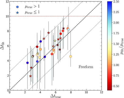
Time delay fits are given for 30 two-image systems, showing that Δt_fit ≈ Δt_true even in the regime 2 d ≤ Δt_true < 8 d, below the threshold used in the main text. The dashed diagonal line gives Δt_fit = Δt_true, while the dotted diagonals give ±2.5 d around this. Error bars show the 95 per cent confidence intervals.

Open in new tabDownload slide