


ABSTRACT
We present new 3-mm continuum and molecular lines observations from the ATOMS survey towards the massive protostellar clump, MM1, located in the filamentary infrared dark cloud (IRDC), G034.43+00.24 (G34). The lines observed are the tracers of either dense gas (e.g. HCO+/H13CO+ J= 1–0) or outflows (e.g. CS J= 2–1). The most complete picture to date of seven cores in MM1 is revealed by dust continuum emission. These cores are found to be gravitationally bound, with virial parameter, αvir < 2. At least four outflows are identified in MM1 with a total outflowing mass of ∼45 M⊙, and a total energy of 1 × 1047 erg, typical of outflows from a B0-type star. Evidence of hierarchical fragmentation, where turbulence dominates over thermal pressure, is observed at both the cloud and the clump scales. This could be linked to the scale-dependent, dynamical mass inflow/accretion on clump and core scales. We therefore suggest that the G34 cloud could be undergoing a dynamical mass inflow/accretion process linked to the multiscale fragmentation, which leads to the sequential formation of fragments of the initial cloud, clumps, and ultimately dense cores, the sites of star formation.
1 INTRODUCTION
High-mass stars (M⋆ > 8 M⊙) are of great importance in many astrophysical processes ranging from the production and transfer of heavy elements via nucleosynthesis, to the structure and evolution of their host galaxies, and even to future star formation in their natal molecular clouds (e.g. Kennicutt 2005; Urquhart et al. 2013). However, high-mass star formation remains poorly understood due to the observational challenges stemming from the relatively large distances to young high-mass stars, their rarity, opaque surroundings, short lifetime, and the complicated, crowded cluster environment (e.g. Zinnecker & Yorke 2007; Tan et al. 2014; Motte, Bontemps & Louvet 2018). High-mass stars are known to form mainly in clusters through hierarchical fragmentation. In both observations and theoretical treatments (e.g. Zhang et al. 2009; Wang et al. 2011; Peretto et al. 2013; Wang et al. 2014; Beuther et al. 2018; Motte et al. 2018; Yuan et al. 2018; Vázquez-Semadeni et al. 2019), hierarchical fragmentation has been observed to proceed on almost all scales from cloud, through filaments and clumps, to individual star-forming cores,1 ultimately leading to a cluster of young stars. Moreover, the entire fragmentation process has been recognized to play a crucial role in determining the final mass of the individual stars formed, and thus the initial mass function, where the latter is a key input to the current theories.
Several efforts have been made to investigate the process of fragmentation, especially on clump and core scales (e.g. Palau et al. 2013, 2014; Csengeri et al. 2017; Beuther et al. 2018; Li et al. 2019, 2020; Sanhueza et al. 2019; Svoboda et al. 2019; Palau et al. 2021). However, finding different degrees of fragmentation makes it difficult to draw a decisive conclusion about the modality of fragmentation, which is a key parameter, especially for high-mass star formation. For example, Csengeri et al. (2017) found a low level of fragmentation with fragment masses above 40 M⊙ in their ALMA-880 |$\mu$|m (i.e. 340.1 GHz) observations of 35 massive clumps down to 0.06-pc scale. In contrast, based on ALMA-1 mm observations towards 12 infrared dark cloud (IRDC) clumps, Sanhueza et al. (2019) revealed a higher level of fragmentation with a large population of low-mass (≤1 M⊙) cores of sizes ≤0.1 pc but no high-mass counterparts (≥30 M⊙). These different degrees of fragmentation probably represent different modalities that control the mass reservoir feeding the individual stars, as predicted by the two main competing theories of high-mass star formation: ‘core-accretion’ (McKee & Tan 2003) and ‘competitive-accretion’ (Bonnell, Vine & Bate 2004). The core-accretion hypothesis, which is essentially a scaled-up version of low-mass star formation, favors the fragmentation of a clump into massive cores that proceed to form high-mass stars. In comparison, the competitive-accretion theory predicts the fragmentation of a clump into a larger population of low-mass cores that competitively accrete from the common mass reservoir. In this framework, cores located at the gravitational well of the system preferentially form high-mass stars. Therefore, more detailed investigation is still needed to establish the link between the observations of the degree of fragmentation and theoretical predictions.
Fragmentation tends to be associated with rich and complex kinematics and dynamics as a result of the interaction among gravity, turbulence, magnetic fields, and/or other factors such as intense radiative feedback from newly formed stars. Both kinematics and dynamics are therefore thought to be useful probes for dissecting the underlying physics (e.g. mass accretion, outflows) related to hierarchical, multiscale fragmentation processes in star formation. Recent state-of-the-art numerical simulations of cloud complexes (e.g. Padoan et al. 2020) have reproduced a web of filamentary structures, each with longitudinal velocity gradient indicative of a mass flow along the filament converging towards the web node, where high-mass young stellar objects (YSOs) are preferentially found to reside. The mass of the final stars has therefore been suggested to be regulated not only by the clump- or core-scale mass accretion but also by the larger scale mass inflow/accretion. In fact, this multiscale mass inflow/accretion has been revealed in previous multiscale kinematic observations (Zhang & Wang 2011; Peretto et al. 2013; Chen et al. 2017; Yuan et al. 2018). For example, in their study of the high-mass protostellar clump, G22, Yuan et al. (2018) observed that the protostar grows in mass simultaneously via core, clump, and cloud-fed accretion with an increasing trend of mass inflow/infall rates of 7.4 × 10⁻⁵ , 7.2 × 10⁻⁴, and ∼100 |$\mathrm{M}_\odot \, \rm yr^{-1}$|, respectively. It thus appears extremely promising to conduct similar studies to obtain an in-depth understanding of the kinematics and dynamics involved in the process of multiscale fragmentation associated with high-mass star formation.
The primary target for this study is the massive clump, MM1, located in the well-known filamentary IRDC, G034.43+00.24 (hereafter G34; Rathborne et al. 2005; Rathborne, Jackson & Simon 2006; Lu et al. 2014; Liu et al. 2020a). We have also probed another associated massive clump, MM2, which is partly covered with the ATOMS survey. We adopt a kinematic distance of 3.7 ± 0.3 kpc (e.g. Rathborne et al. 2005; Xu et al. 2016; Tang et al. 2019; Liu et al. 2020a) to this cloud. The two massive clumps have a few hundred solar masses within diameters of 0.2–0.5 pc. MM1 has a bolometric luminosity of 2.4 × 10⁴ L⊙ mainly due to an associated B0-type YSO (Fig. 1), while MM2 has a bolometric luminosity of 1.4 × 10⁴ L⊙ mainly from an associated ultracompact H ii region (UC-H ii, i.e. IRAS 18507+0121, Bronfman, Nyman & May 1996). The coexistence of these star-forming signatures and the IRDC nature of the G34 cloud suggests early stages of high-mass star formation in the clumps, MM1 and MM2.
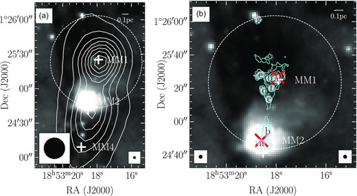
Panel (a): the two massive protostellar clumps, MM1 and MM2, of IRDC G34 in Spitzer 8.0-μm image overlaid with the ATLASGAL 870-μm continuum contours. The contours start at 3 rms (rms ∼0.6 Jy beam−1) increasing in steps following the power-law D = 3 × Np + 2, where D is the dynamical range of the intensity map (i.e. the ratio between the peak and the rms noise), N is the number of contours used (8 in this case). The millimeter clumps identified from the 1.2-mm continuum maps presented by Rathborne et al. (2006) are indicated with plus symbols. The beams of the 8.0- and 870-μm data are shown at the bottom left-hand, and bottom right-hand corners, respectively. Panel (b): close-up view of MM1 and MM2. The contours represent the ATOMS 3-mm continuum emission. Note that the ATOMS map is not corrected for the primary beam. The contour levels start at 3 rms (rms ∼0.3 mJy beam−1) with steps following the same power-law form as in panel (a). Labels (a)–(g) identify the cores extracted from the continuum emission. The beams of the 8.0-μm and 3-mm data are shown at the bottom left-hand, and bottom right-hand corners, respectively. The locations of the B2-type YSO associated with MM1 and the UC-H ii region associated with MM2 are indicated with red X symbols. The dashed circle in both panels demarcates the field view of the ATOMS 3-mm observations.
In this paper, we present our new ALMA 3-mm observations towards IRDC G34, which is part of the ATOMS survey2 (Project ID: 2019.1.00685.S, Liu et al. 2020b,c, 2021, hereafter Paper I, Paper II, and Paper III, respectively, see Section 2). The ATOMS survey is aimed to investigate statistically the relation between high-mass star formation and the distribution of dense gas, filamentary structures, and feedback, by observing 3-mm continuum and gas emission at a nearly uniform angular resolution of ∼2 arcsec towards a sample of 146 high-mass star-forming IRAS regions in the range −80○ < l < 40○ and |b| < 2○ (Bronfman et al. 1996; Faúndez et al. 2004). The overview paper (Paper I) presents the source sample, the spectral setup, and the major goals of the survey. Paper II addresses the relation between high-mass star formation and the dense gas distribution by investigating the star formation scaling relations inferred from different dense gas tracers (e.g. HCO+/H13CO+, HCN/H13CN). Paper III includes the catalogues of candidate hot molecular cores and hyper/ultracompact H ii regions, which provide an important foundation for future studies of the early stages of high-mass star formation across the Milky Way.
In this paper, we make full use of the ATOMS data to gain insight into the fragmentation and dynamical processes of the G34 cloud through observations of its two massive, luminous protostellar clumps, MM1 and MM2. This paper is organized as follows: Section 2 gives a brief description of the ALMA observations of the ATOMS survey, Section 3 presents analysis of the ATOMS data, Section 4 discusses the observed hierarchical fragmentation and the associated dynamical mass inflow/accretion scenario, and Section 5 summarizes the results.
2 ALMA OBSERVATIONS AND DATA REDUCTION
Observations of the ATOMS survey consist of single pointings towards 146 IRAS clumps by both the Atacama Compact 7-m Array (ACA; Morita Array) and the 12-m array (C43-2 or C43-3 configurations) in Band 3. Eight spectral windows (SPWs) were optimised to cover 11 commonly used lines that includes the tracers of dense gas (e.g. HCO+/H13CO+), hot molecular core gas (e.g. CH3OH), shocked gas (e.g. SiO, and SO), and ionized gas (e.g. H40α). The basic parameters (e.g. rest frequency, transition) of these lines are listed in table 2 of Paper I. The SPWs 1–6 are located at the lower sideband in the range [86.31, 99.40] GHz with spectral resolution of ∼0.2–0.4 km s−1 for kinematic measurements, while SPWs 7–8 in the upper sideband in the range [99.46, 101.34] GHz each has a broad bandwidth of 1875 MHz at a spectral resolution of ∼1.6 km s−1 for sensitive continuum measurements.
The data were calibrated in casa 5.6 (McMullin et al. 2007). We then imaged and cleaned the ACA and 12-m-array data jointly using natural weighting (to optimize the signal-to-noise ratio) and taking pblimit = 0.2, in the casa tclean task, for both continuum images and line cubes. Continuum images were created from line-free frequency ranges of SPWs 7–8 centred at ∼99.4 GHz while the spectral line cube of each SPW was produced with its native spectral resolution. The resulting continuum image and line cubes for the 146 target clumps have angular resolutions ∼1.2–1.9 arcsec, and maximum recoverable angular scales ∼60 arcsec.
In this paper, we analyse the I18507+0121 source from the ATOMS, whose ALMA observations cover the MM1 and MM2 clumps of G34. The analysis presented is carried out on the combined data sets unless specified otherwise. The 12m+ACA combined continuum image of this source has a beam size of 1.9 × 2.1 arcsec2, and a sensitivity of 1rms = 0.3 mJy beam−1, which corresponds to a mass sensitivity of ∼0.1 M⊙ at the distance of the source for a dust temperature of ∼20 K (see Section 3.1 for the detailed mass calculation). For line cubes, only the HCO+ (1–0), H13CO+ (1–0), SiO (2–1), SO (3–2), CS (2–1), and CH3OH 2(1, 1)–1(1, 0)A lines are utilized for investigating the kinematics and dynamics of MM1 and MM2. The velocity resolutions for the HCO+, H13CO+/SiO, and SO/CS/CH3OH lines are 0.1, 0.2, and 1.5 km s−1, respectively, and the sensitivity levels are ∼12, 8, and 3 mJy beam−1, respectively.
3 RESULTS AND ANALYSIS
3.1 3-mm continuum emission
Fig. 1 illustrates the overall morphology and location of the MM1 and MM2 protostellar clumps of G34 in the Spitzer 8.0-μm image overlaid with ATLASGAL 870 |$\mu$|m dust continuum in panel (a), and with the ATOMS 3-mm continuum data in panel (b). The ATOMS continuum image presented in this figure and Fig. 2 is not corrected for the primary beam response. This is done only for the purpose of display since it enables a uniform noise level to be shown in the map. But for the analysis of the core properties, the primary-beam corrected 3-mm image is used (see Paper III for more details). The dashed circle in Fig. 1(a) marks the field of view (80 arcsec in diameter) of the resulting combined image of ATOMS used in this study. As seen, the MM1 clump is fully covered while only half of the MM2 area is observed by the ATOMS. The large-scale filamentary cloud overall appears dark against the background emission at 8 |$\mu$|m. Also marked in the figure is the chain of the three millimeter clumps (i.e. MM1, MM2, and MM4), identified by Rathborne et al. (2006) from 1.2-mm continuum observations. The orientation of the clumps along the filament is seen to be replicated on smaller scales as well, as is evident from the north–south spread of the detected cores in the 3-mm continuum of the ATOMS data. The 3-mm continuum emission observed across the entire region mainly comes from thermal dust emission since ATOMS detected no H40α emission. Further, only two very compact centimetre sources of size ∼1 arcsec are detected by Rosero et al. (2016), which are confined within the centres of the MM1 and MM2 clumps.
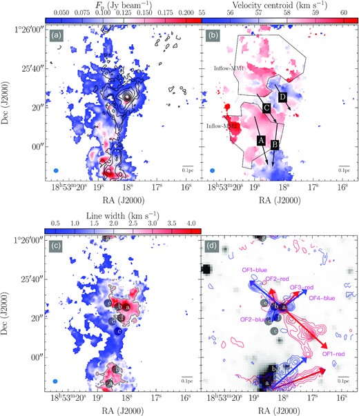
Panel (a): peak intensity map of H13CO+ (1–0) for the MM1 and MM2 protostellar clumps in G34. The 3-mm dust continuum emission is shown in black contours, starting at 3 rms (rms ∼0.3 mJy beam−1) with the steps following the same power-law form as in Fig. 1. Panel (b): moment 1 map of H13CO+ (1–0). The arrows A–D mark the directions of the observed velocity-coherent gradients. The polygons represent the gas inflow regions for each cluster of cores in MM1 and MM2. Panel (c): line width map of H13CO+ (1–0). The contour represents a line width of 2.5 km s−1. Panel (d) CS (2–1) outflows (contours) superimposed on the Spitzer 4.5-μm image. The red and blue arrows indicate the red and blue lobes of outflows, respectively. Labels a–g in panels (c) and (d) identify the dense cores in MM1 and MM2 protostellar clumps. In all panels, the map is displayed only at the positions where the peak intensity of the spectrum is ≥5 times the local noise level.
The high angular resolution of the ATOMS 3-mm continuum map allows to identify the dense cores where stars form. Paper III adopted a combination of the Dendrogram algorithm and casa-imfit function to extract cores. As discussed by these authors, the former technique does not always provide good measurements of the core parameters on size and position angle, while the latter performs better in this regard through a two-dimensional Gaussian fit to the emission. Following this approach, nine cores are extracted from the 3-mm continuum map with seven (i.e. MM1a–g, see Fig. 1b) in MM1 and two (i.e. MM2a–b) belonging to MM2. Note that the MM1-b core was manually located and then extracted with casa-imfit since it was not automatically detected by Dendrogram due to its close proximity and small intensity contrast relative to the neighbouring MM1-a core. The additional extraction of MM1-b was driven by the associated outflows (see Fig. 2d). Its existence was further verified through a careful visual examination of the radial intensity profile along the direction connecting both MM1-b and MM1-a sources, where the weak and strong intensity peak components correspond to the two sources, respectively.
Overall, the result of core extraction in this work matches that of Paper III with the exception of the two cores, MM1-g, and MM2-a. Both of them are located outside a circle of radius 36 arcsec around the image centre, which was imposed as a mask for batch extraction of cores from all of the 146 ATOMS clumps, and thus ignored in Paper III. Our ATOMS observations have revealed the most complete population of cores (i.e. a cluster of seven cores) in MM1, compared with the previous SMA observations (e.g. Rathborne et al. 2011), in which only the MM1-a core was revealed. This could be a consequence of either the missing-flux effect due to the limited uv coverage by SMA or the poor sensitivity. Additionally, due to the incomplete coverage by the ATOMS for MM2, we believe that the population of cores in this clump has not been fully unveiled, and this clump could also be harbouring a cluster of cores.
The measured parameters of the nine cores are listed in Table 1, including the deconvolved sizes of the major and minor axes (Column 4), the position angle (Column 5), the core-integrated 3-mm flux (Column 6), and the core-peak flux (Column 7). Note that both MM1-a and MM2-a cores have an associated compact centimeter source, each with a size of ∼1 arcsec. The two sources coincide with an early B-type star in MM1 (see Fig. 1; Shepherd et al. 2007), and an UC-H ii region in MM2. In addition, the centimetre sources in MM1-a and MM2-a correspond to partially optically-thick free–free emission and non-thermal emission, respectively, with the former having a spectral index of α = 0.7 in the frequency range 4.9–25.5 GHz and the latter having α = −0.5 (Rosero et al. 2016). Given a total flux density of ∼0.4 and 9.5 mJy at 4.9 GHz for the centimeter sources in MM1-a, and MM2-a, respectively, the relation Sν∝να yields a flux density of ∼3 and 2.1 mJy, respectively, at 3 mm, which is negligible compared to the total fluxes of the two cores.
Continuum core parameters.
| Name | RA | Dec. | FWHMDec. | PA | |$F_{\rm 3\,mm}^{\rm int.}$| | |$F_{\rm 3mm}^{p}$| | Rcore | Tgas | Mcore | log(ncore) | Σcore | Vlsr | ΔV | αvir |
|---|---|---|---|---|---|---|---|---|---|---|---|---|---|---|
| (J2000) | (J2000) | maj(arcsec) × min(arcsec) | (°) | (mJy) | (mJy beam−1) | (10−2 pc) | (K) | (M⊙) | (cm−3) | (g cm−2) | (km s−1) | (km s−1) | ||
| MM1-a | 18:53:18.02 | 1:25:25.7 | 2.3 × 2.2 | 21.4 | 124.2 ± 0.8 | 54.7 ± 0.2 | 2.0 ± 0.2 | 100.0 | 199 ± 32 | 7.4 | 32.7 | 57.6 ± 0.2 | 4.5 ± 0.2 | 0.5 |
| MM1-b | 18:53:18.29 | 1:25:25.9 | 2.2 × 2.0 | 102.1 | 9.6 ± 0.1 | 9.6 ± 0.2 | 1.9 ± 0.2 | 27.6 | 58 ± 9 | 7.3 | 11.0 | 57.1 ± 0.2 | 2.9 ± 0.2 | 0.6 |
| MM1-c | 18:53:18.30 | 1:25:13.6 | 3.5 × 2.4 | 16.0 | 9.1 ± 1.0 | 2.8 ± 0.2 | 2.6 ± 0.2 | 14.2 | 115 ± 19 | 7.0 | 11.1 | 59.3 ± 0.2 | 1.1 ± 0.2 | 0.1 |
| MM1-d | 18:53:18.50 | 1:25:18.4 | 3.8 × 2.5 | 32.0 | 10.3 ± 1.0 | 3.0 ± 0.2 | 2.7 ± 0.2 | 13.8 | 136 ± 22 | 7.0 | 12.1 | 58.6 ± 0.2 | 1.8 ± 0.2 | 0.1 |
| MM1-e | 18:53:18.64 | 1:25:28.0 | 4.5 × 3.5 | 112.9 | 5.6 ± 0.1 | 1.9 ± 0.2 | 3.5 ± 0.3 | 22.6 | 42 ± 7 | 6.5 | 2.2 | 57.4 ± 0.2 | 1.6 ± 0.2 | 0.5 |
| MM1-f | 18:53:18.19 | 1:25:20.3 | 2.7 × 2.1 | 152.5 | 6.9 ± 0.1 | 5.5 ± 0.2 | 2.1 ± 0.2 | 18.6 | 65 ± 11 | 7.2 | 9.5 | 56.9 ± 0.2 | 3.3 ± 0.2 | 0.8 |
| MM1-g | 18:53:18.71 | 1:26:1.3 | 3.7 × 1.6 | 151.0 | 24.5 ± 0.9 | 9.1 ± 0.2 | 2.1 ± 0.2 | 21.7 | 196 ± 32 | 7.4 | 28.3 | 58.4 ± 0.2 | 3.4 ± 0.2 | 0.3 |
| MM2-a | 18:53:18.60 | 1:24:46.7 | 5.3 × 4.0 | 23.2 | 62.3 ± 1.5 | 9.8 ± 0.2 | 4.1 ± 0.3 | 100.0 | 97 ± 16 | 6.4 | 3.8 | 56.5 ± 0.2 | 2.5 ± 0.2 | 0.7 |
| MM2-b | 18:53:18.38 | 1:24:54.1 | 6.7 × 2.9 | 0.8 | 34.0 ± 1.4 | 5.5 ± 0.2 | 3.9 ± 0.3 | 20.8 | 281 ± 46 | 6.9 | 12.2 | 56.2 ± 0.2 | 2.7 ± 0.2 | 0.2 |
Note. Rcore is derived from Reff/3600 × π/180 × D given the relation |$R_{\rm eff} = \sqrt{FWHM_{\rm dec}^{\rm maj}\times FWHM_{\rm dec}^{\rm min}}/2$|, and the distance D of the core. Gas temperature for all the cores, except for MM1-a and MM2-a, is estimated from the kinetic temperature map obtained from VLA observations of NH3 by Lu et al. (2014). For cores MM1-a and MM2-a, the temperature is assumed to be 100 K, given their association with a hot molecular core and an UC-H ii region, respectively. Vlsr and ΔV along with the associated errors are derived from single Gaussian component fit to the average spectrum of H13CO+ (1–0) over each core. The errors for the fluxes result from the 2D Gaussian fitting in the core extraction, while the ones for Rcore, Mcore, and ncore are mainly due to the distance uncertainty.
The mass, Mcore, and the column density, Ncore, of the cores were calculated following equations (B1)– (B2) of Paper III. In the calculation, the gas temperature for all the cores, except for MM1-a and MM2-a, is estimated from the kinetic temperature map obtained from the VLA 3-arcsec-resolution observations of the NH3 (1, 1) and (2, 2) inversion lines by Lu et al. (2014). For MM1-a and MM2-a, the temperature is assumed to be 100 K due to the presence of an associated hot molecular core, and an UC-H ii region (Rathborne et al. 2011, Paper III), respectively. In addition, a gas-to-dust mass ratio of Rgd = 100 was adopted. Recent works propose higher values (|$R_{\rm gd}^{\prime }$|) like 150 (Draine 2011) or 162 (Peters et al. 2017). One can estimate Mcore and Ncore with different gas-to-dust mass ratios simply by multiplying a scaling factor of |$R_{\rm gd}^{\prime }/R_{\rm gd}$|. In the above calculation, the core flux includes background emission, which could lead to the overestimation of the core masses. In practice, the background emission is difficult to be accurately subtracted especially from the high-resolution ATOMS data that have already filtered out a significant portion of large-scale components. For a conservative estimate, we assume a constant value of 1 rms level for the background emission. Using this, it is seen that the median value of the new core masses decreases by |$\sim \! 25{{\ \rm per\ cent}}$| where the decrease in mass is mostly seen in the relatively low-density cores while the more massive and dense ones remain more or less unchanged.
Furthermore, the mass surface density can be derived from |$\Sigma _{\rm core} = M_{\rm core}/(\pi R_{\rm core}^2)$|, while the number density from ncore = Ncore/2Rcore, where Rcore is the core radius equal to the geometric mean of |$FWHM_{\rm maj}^{\rm Dec.}$| and |$FWHM_{\rm min}^{\rm Dec.}$| at the core distance. The above derived parameters can be found in columns 9–11 of Table 1. In summary, we find Rcore ∼ 0.02–0.04 pc with a median value of 0.03 pc, Mcore ∼ 42–281 M⊙ with a median value of 115 M⊙, ncore ∼ 0.2 × 10⁷–2.8 × 107 cm−3 with a median value of 1.1 × 107 cm−3, and Σcore ∼ 2–32 g cm−2 with a median value of 11 g cm−2. If a theoretical threshold of 1 g cm−2 above which the cores most likely form high-mass stars, is assumed (Krumholz & McKee 2008), then the entire population of cores detected in this study have the ability to form high-mass stars.
Following the method described above, we also estimated the mass, Mcl, and the number density, ncl, of the G34 cloud (80 arcsec in size) considering the region within the field of view of the ATOMS observations. Since the kinetic temperature map of Lu et al. (2014) is obtained using interferometric observations, structures with spatial scales larger than that of the ATOMS cores are resolved out. Hence, for these calculations, we assume a cloud-average dust temperature of ∼21 K, which was measured over the field of view of the ATOMS observations from the publicly available dust temperature map created using the point processing mapping (PPMAP) technique, a state-of-the-art spectral energy distribution fit method (Marsh et al. 2017). The assumption of this temperature is in good agreement with the cold nature of the IRDC cloud (e.g. Carey et al. 1998, 2000; Rathborne et al. 2006; Soam et al. 2019). Taking the integrated flux of 480 Jy at 870 |$\mu$|m from the ATLASGAL image of the cloud leads to Mcl ∼ 4.2 × 10⁴ M⊙, and ncl ∼ 2.6 × 105 cm−3. The mass conversion efficiency from cloud to cores is rather low at about |$3{{\ \rm per\ cent}}$|, although the masses of the cores are far above the mass sensitivity (i.e. ∼0.3 M⊙ for a 3- rms detection) of the observations, implying that most of the cloud gas is not efficiently transformed into cores.
3.2 Molecular gas emission
The average spectrum of H13CO+ (1–0) over the entire region investigated here reveals a systemic velocity of Vlsr = 57.6 km s−1. In general, H13CO+ emission is treated as relatively optically thin. However, this may not be the case for the densest part of cores. Following equation (1) of Liu et al. (2020a), we calculate the optical thickness from the peak intensity of H13CO+ of the nine cores with the assumptions of local thermodynamic equilibrium (LTE). This yields optical depth values in the range of 0.04–0.39 and hence supports the optically thin assumption for the H13CO+ emission. Besides, extended emission of H13CO+ appears as a single-peaked spectral profile across the entire region at a high spectral resolution 0.2 km s−1, which makes the H13CO+ (1–0) line a good probe for the spatial distribution of molecular gas within the MM1 and MM2 clumps.
Fig. 2(a) displays the map of the peak intensity of H13CO+ (1–0). For comparison, the 3-mm dust continuum is also overlaid as contours in the figure. H13CO+ (1–0) gas and 3-mm dust continuum distribution are found to match each other well in dense regions, with the former being much more extended than the latter across the entire region. In particular, a bright branch of H13CO+ emission, which appears to stretch towards the cluster of cores (MM2a–b) in MM2, does not have detectable continuum emission at the current sensitivity. The non-detection of dust continuum indicates that this branch of H13CO+ emission could be ambient gas having lower column density than that concentrated in the clusters of cores with apparent dust emission.
Fig. 2(b) presents the moment 1 map of H13CO+ (1–0) that can reveal the global velocity field. Velocity gradients can be seen towards the cluster of cores in both MM1 and MM2. In particular, the velocity gradients towards the cluster of cores in MM2 appear to match the bright branch of H13CO+ gas emission mentioned above, suggesting that ambient gas is being accelerated by the gravity of the cluster of cores in MM2, and thus inflowing towards them (see Section 4.2 for additional discussion). Quantitatively, the velocity gradients are evaluated along the four directions (indicated by arrows A–D in Fig. 2b). These four directions are visually identified after a careful examination of the moment 1 map. We find from Fig. 3 that the gradients lie in the range of ∼3–8 km s−1 pc−1. Of particular interest is the gradient along the direction D, which appears to be the signature of rotational motion (see Section 3.5 for more analysis).
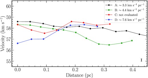
Velocity distribution derived from H13CO+ (1–0) along the four selected directions A–D, which are indicated in Fig. 2(b). The typical error bar of the velocity gradient is shown at the bottom right-hand side.
Fig. 2(c) shows the line width map of H13CO+ (1–0) reflecting the global kinematics of the entire region investigated here. The line width tends to be enhanced around the centres of the clusters of cores in both MM1 and MM2. Given that the H13CO+ (1–0) emission is seen to be optically thin, the effect of optical depth can be ruled out and this enhancement can be attributed to intense star-forming feedback (e.g. energetic outflows and stellar winds) due to the presence of the luminous YSO in MM1 and the UC-H ii region in MM2 (Shepherd et al. 2007; Liu et al. 2020a). Moreover, the dynamical motions of the gravity/turbulence-driven inflows toward the centres of MM1 and MM2 can be an additional source for the enhanced line width.
To quantitatively describe this enhancement, we plot, in Fig. 4, the distribution of the line widths for the entire region. A distinct inflection at the line width of ∼2.5 km s−1 is evident on visual inspection of the distribution. This turnover could represent the threshold above which the line width is enhanced by strong feedback from star formation and probably by the dynamical gas inflows, and below which the gas kinematics are less affected. This threshold can also be found in Fig. 2(c) where the threshold of ∼2.5 km s−1 (in grey contour) does separate the weak- and strong-feedback areas well. The mean line width is ∼2.9 km s−1 in the area of strong feedback, and ∼1.3 km s−1 elsewhere.
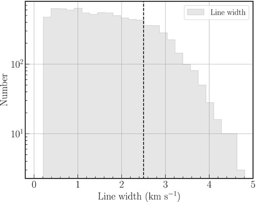
Distribution of the line widths derived from H13CO+ (1–0). The y-axis shows the number of pixels. An inflection in the distribution can be found at ∼2.5 km s−1(indicated by the dashed vertical line).
3.3 Molecular outflows
Previous single-dish as well as interferometric observations have shown the presence of outflows in the MM1 and MM2 clumps (e.g. Rathborne et al. 2011; Zhang et al. 2014; Liu et al. 2020a). With the new observations from the ATOMS survey that include several commonly used outflow tracers like HCO+, CS, SiO, SO, and CH3OH, we identify, in different tracers, the outflows associated with the two clusters of cores in MM1 and MM2. In the identification, the outflowing gas velocities of each tracer (line) are taken from the line wings of its spectrum, which lie outside the full width of half-maximum of the spectrum. The spectrum used is averaged over the entire region investigated here. The blue and redshifted outflowing gas emission, in sequence, is integrated over the velocity ranges (1) [44.0, 55.0] and [60.0, 76.0] km s−1 for HCO+ (1–0), (2) [40.0, 51.4] and [63.4, 82.0] km s−1 for CS, (3) [42.0, 51.3] and [63.5, 74.0] km s−1 for SiO, (4) [42.0, 52.7] and [62.2, 78.0] km s−1 for SO, and (5) [46.0, 54.2] and [60.6, 66.0] km s−1 for CH3OH.
In total, six outflows are identified with four within the MM1 clump (i.e. MM1-OF1 to MM1-OF4) and two within MM2. All of the outflows are identifiable in the five tracers with the exception of MM1-OF3, which is visible only in CS and SiO emission. The outflows identified with each tracer are plotted in Figs 2(d) and A1. For comparison, the Spitzer 4.5 |$\mu$|m is overlaid, which is thought to be an indicator of shocked gas. As seen, the outflow gas extent does not correspond to the extended 4.5-|$\mu$|m emission well. From the figure, MM1-OF1/OF3/OF4 appear to be driven by the embedded source(s) in MM1-a while MM1-OF2 by the source(s) in MM1-b. In MM1, all of the outflows except for MM1-OF1 are distinct from the results of Shepherd et al. (2007). The low-resolution (angular resolution of 3.6 arcsec) CO (1–0) observations presented by these authors do not reveal the presence of MM1-OF2 nor do they distinguish between the MM1-OF3 and MM1-OF4 outflows. Although both MM1-OF3 and MM1-OF4 outflows display single lobes, these have a high possibility of being associated with the MM1-a core due to the outflowing velocities ranging around the systemic velocity of MM1-a.
In a later study by Isequilla et al. (2021), based on higher 0.8-arcsec-resolution observations of CO (2–1), the two lobes of MM1-OF2 were reported as separate outflows but not as a bipolar outflow. Since the driving source(s) of the outflows within MM2 (i.e. MM2-OF1/OF2) could not be probed due to the incomplete coverage of ATOMS, they are not considered for further analysis. In addition, we find that the outflows identified with the new observations are more collimated than those seen from the CO (1–0) observations by Shepherd et al. (2007), suggesting that the outflow tracers used here, that have much higher critical density than CO (1–0), could be probing the compact, highly-collimated jets.
3.4 Outflow parameters in MM1
Parameters such as the momentum, dynamical age, and ejection rate are valuable for characterizing the outflows. In principle, both CS and SiO emission can be used for the calculation since from Figs 2(d) and A1 they both are found to trace the extent of all of the outflows better than the other three tracers. Since the shock-sensitive SiO is preferentially enhanced in shocked regions, and less abundant elsewhere, the core-scale abundance is required to more properly estimate the abundance-related parameters like the momentum. Since no core-scale measurement of SiO abundance is available for the cluster of cores in MM1, we consider CS emission only, which can be abundant in non-shocked as well as shocked regions, and in general is not as sensitive to shocked gas as SiO emission.
Following Shepherd et al. (2007), an inclination angle of 45 ○ was assumed for simplicity, which minimizes the errors introduced by inclination effects for outflows with unknown orientation. The total outflowing gas mass, Mout, was inferred from ΣMi, where the gas mass, Mi, in the velocity channel i was calculated from equation (4) of Liu et al. (2020a) assuming optically-thin emission, LTE conditions, and a CS abundance of 5.8 × 10⁻¹⁰ inferred by Liu et al. (2020a). In addition, the clump-average dust temperature of 38 K as quoted in Liu et al. (2020a) was taken as the excitation temperature in the calculation. The momentum, Pout, was derived from ΣMivi and the kinetic energy, Eout, from |$({1}/{2}) \Sigma M_{i} v_{i}^2$|, with vi defined as the central velocity of the ith channel relative to Vlsr. The dynamical age, tdyn, was estimated from |$\langle$|L|$\rangle$|/|$\langle$|V|$\rangle$|, where |$\langle$|L|$\rangle$| is the average length of the red and/or blue lobes of outflows and |$\langle$|V|$\rangle$| is the intensity-weighted mean velocity defined as Pout/ΣMi. Accordingly, the outflowing mass rate, |$\dot{M}_{\rm out}$|, is given by ΣMi/tdyn, and the mechanical force, Fout, by Pout/tdyn.
Table 2 summarizes the above-derived parameters for the CS outflows within MM1. The parameter errors mainly arise from the uncertainties of the distance and/or velocity measurements. The global properties of all of the outflows in MM1 (e.g. Mout, and Pout) agree with those derived from CO (1–0) interferometric observations by Shepherd et al. (2007), who treated all outflows in MM1 as a single outflow. Further, the estimated dynamical ages of all outflows suggest that MM1-OF1 is the oldest while the lifetimes of MM1-OF2/OF3/OF4 are comparable, whereas all of the outflows are very young with respect to the average dynamical time of order of 104 yr over near 400 molecular outflows catalogued by Wu et al. (2004).
CS (2–1) outflow parameters.
| Outflow | Lobes | |$\langle$|L|$\rangle$| | |$\langle$|V|$\rangle$| | Mout | Pout | Eout | Fout | tdyn | |$\dot{M}_{\rm acc}$| |
|---|---|---|---|---|---|---|---|---|---|
| (pc) | (km s−1) | (M⊙) | (102M⊙ km s−1) | (1046erg) | (10−3M⊙ km s−1 yr−1) | (103 yr) | (10−5M⊙ yr−1) | ||
| MM1-OF1 | B+R | 0.47 ± 0.07 | 14.6 ± 1.5 | 34.9 ± 1.7 | 5.1 ± 0.3 | 7.8 ± 0.4 | 16.2 ± 5.0 | 3.1 ± 0.8 | 3.0–6.0 |
| MM1-OF2 | B+R | 0.18 ± 0.03 | 14.9 ± 1.5 | 8.0 ± 0.4 | 1.2 ± 0.1 | 1.8 ± 0.1 | 10.1 ± 3.3 | 1.2 ± 0.3 | 2.0–4.0 |
| MM1-OF3 | R | 0.23 ± 0.02 | 18.2 ± 1.8 | 1.8 ± 0.1 | 0.3 ± 0.1 | 0.6 ± 0.1 | 2.6 ± 0.6 | 1.3 ± 0.2 | 0.4–0.7 |
| MM1-OF4 | B | 0.14 ± 0.01 | 12.0 ± 1.2 | 1.1 ± 0.1 | 0.1 ± 0.1 | 0.2 ± 0.1 | 1.1 ± 0.3 | 1.2 ± 0.2 | 0.2–0.3 |
| Total | – | – | – | 44.7 ± 1.7 | 6.6 ± 0.3 | 10.2 ± 0.4 | 29.0 ± 5.0 | – | 5.4–10.7 |
Note. B and R in Column 2 stand for the blue and red lobe of outflows, respectively.
If we assume momentum-driven outflows in protostellar-jet/outflow systems (e.g. Masson & Chernin 1993; Goddi et al. 2020) along with momentum conservation, the relation |$\dot{M}_{\rm jet} V_{\rm jet} = \dot{M}_{\rm out} V_{\rm out} = F_{\rm out}$| follows, where |$\dot{M}_{\rm jet}$| and Vjet are the mass-loss rate and the speed of the jet, respectively. The jet speed for massive outflows was observationally measured to be around 500 km s−1 in several proper motion studies of radio continuum jets (e.g. Marti, Rodriguez & Reipurth 1995). In protostellar jet/outflow systems, the ejection rate is expected to correlate with the accretion rate via the relation |$\dot{M}_{\rm acc} = (1+f_{\rm jet})/f_{\rm jet} \times \dot{M}_{\rm jet}$|. The fraction fjet, defined as the ratio between the accretion mass rate and the mass-loss rate through the jet, is poorly constrained by observations, but predicted in models to be 0.2–0.5 (e.g. Offner & Arce 2014; Kuiper, Turner & Yorke 2016). This fjet range yields a range of the mass accretion rates for each outflow (last column of Table 2). If all of the outflows in MM1 are treated as a single entity, the total mass accretion rate on to the protostars will be in the range [5, 11]× 10−5 M⊙ yr−1, which is in agreement with rates estimated for other high-mass star-forming systems (e.g. Zhang et al. 2005, 2013; Yuan et al. 2018)
3.5 A rotating envelope within MM1?
The extended H13CO+ emission presents a clear south-west-north-east (SW-NE) velocity gradient (i.e. along the direction D in Fig. 2b), with redshifted emission to the SW and blueshifted emission to the NE of the MM1-a core. This observed velocity gradient has already been reported in higher 0.6-arcsec-resolution observations of CH3OH at ∼345 GHz with SMA by Rathborne et al. (2011, see the right panel of their fig. 6). Ruling out the possibility of the influence from the large-scale MM1-OF1 outflow, these authors interpreted the velocity gradient as arising from a rotating structure surrounding the protostar(s) embedded in the core. Note that the SW-NE velocity gradient shown here is seen only in emission of H13CO+ but not in other species including the complex organic molecules (COMs), such as CH3OH, which are hot-gas tracers. This could perhaps be attributed to either the different transitions involved or the different spatial resolutions of the two data sets. For example, the transition responsible for CH3OH emission at ∼90 GHz in the ATOMS data has a much lower upper energy temperature (∼20 K) than that of the transition of CH3OH at ∼345 GHz where the temperature is >100 K. The CH3OH emission at ∼90 GHz could therefore be tracing different physical regions than those by CH3OH at ∼345 GHz. Besides, the resolution of the ATOMS ∼2 arcsec (corresponding to ∼0.035 pc at the distance of the G34 cloud) is around 3.3 times lower than that of the SMA observations of Rathborne et al. (2011), and hence, the CH3OH emission of the ATOMS may not be able to resolve the velocity structure at the small-scale, local area of hot gas of around 0.004 pc as revealed in Rathborne et al. (2011).
To better understand the velocity distribution along the direction of the velocity gradient (i.e. direction D in Fig. 2b), we plot the position–velocity diagram in Fig. 5. It reveals a typical butterfly-shaped appearance that is characteristic of Keplerian rotation pattern, which might be another indication of the existence of a rotating envelope. Quantitatively, the velocity pattern can be fitted with a Keplerian rotation curve around an Msin2θ ∼10–50 M⊙ protostar, where θ is defined as the inclination angle between the rotation axis and the line of sight. Although this range of masses is consistent with the luminosity (104.3 L⊙) and spectral type (B0) determined from the SED of the MM1-a core by Rathborne et al. (2006), it is still rather small compared with the core’s mass (∼200 M⊙, see Table 1) and is inconsistent with the assumption of the Keplerian rotation that requires the gas mass to be negligible with respect to the central mass (e.g. Cesaroni et al. 2019). This inconsistency can be alleviated if the rotating envelope is sufficiently inclined. For example, if Msin2θ ∼10 M⊙, the stellar mass can exceed the core mass of 200 M⊙ for θ < 13○.
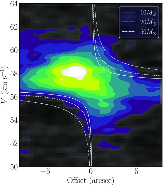
Position velocity diagram of H13CO+ (1–0) for G34–MM1. The position offset is along the D direction indicated in Fig. 2(b). Overlaid on the image are models for Keplerian rotation with central masses of 10, 20, and 50 M⊙.
The mass discrepancy can also be addressed if one considers the mass of ∼8 M⊙ of the more concentrated ∼0.02-pc diameter core, as defined by Rathborne et al. (2011), rather than the large mass of the MM1-a core ∼0.04 pc in diameter estimated with the ATOMS data. Even if this is the case, the rotating structure is too large, around 10 arcsec (0.18 pc), to be arising from an accretion disc, which is generally observed to have a size of a few hundred aus (e.g. Rathborne et al. 2011; Moscadelli et al. 2021). We therefore suggest that the large-scale velocity-coherent gradient revealed in H13CO+ emission could be ascribed to a relatively large, rotating structure.
3.6 Virial analysis
3.7 Jeans length and Jeans mass
Fig. 1 clearly shows fragmentation on two different scales of the cloud and clumps. On the cloud scale, the fragmentation proceeds with ∼0.7 -pc-separated fragments of masses 200–500 M⊙ (clumps MM1, MM2, and MM4 in Fig. 1a), where the fragment masses are from table 1 of Liu et al. (2020a) and the fragment separation is the averaged distance between neighbouring clumps. On the core scale, the fragmentation is evidenced by ∼0.12-pc-separated fragments of typical mass 115 M⊙, where only the fragments (cores) within MM1 are considered, since the population of cores in MM2 suffers from the incomplete coverage in the ATOMS. In this case, the typical mass of the fragments is taken to be the average mass of the cores within MM1, while the typical separation between fragments is determined from the minimum spanning tree technique (e.g. Dib & Henning 2019), which determines the shortest distances that can possibly connect each of the cores in the sampled field.
For the estimate of Jeans parameters on the cloud scale, we assume a gas kinetic temperature of ∼21 K, which corresponds to the average dust temperature over the entire cloud region investigated here (see Section 3.1), and a line width of |$\Delta \, V_{\rm H^{13}CO^{+}}=1.3$| km s−1, which is a typical value of the weak-feedback cloud area (see Fig. 2c and Section 3.2), and thus more representative of the initial turbulence of the cloud than the line widths found in the relatively strong-feedback areas. Following Liu et al. (2019), σth is estimated from the gas kinetic temperature and σnt is determined from |$\Delta \, V_{\rm H^{13}CO^{+}}$|. Finally, using the cloud-average density, ncl ∼ 2.6 × 105 cm−3 (i.e. |$\rho _{\rm eff}^{\rm cl}\sim 4.4\times 10^{-19}$| g cm−3), both thermal and turbulent Jeans parameters are calculated on the cloud scale. Likewise, both thermal and turbulent Jeans parameters on the clump scale can be estimated assuming the same values of gas temperature and line width values as above. This assumption is valid if both cloud- and clump-scale fragmentation occur sufficiently early that the cloud is free of strong star formation feedback. In this case, the mean density of the clump, nclump ∼ 4.9 × 105 cm−3 (Liu et al. 2020a, i.e. |$\rho _{\rm eff}^{\rm clump}\sim 8.2\times 10^{-19}$| g cm−3) is adopted.
Table 3 summarizes the derived Jeans parameters at both cloud and clump scales. At the cloud level fragmentation, the predicted thermal Jeans length is a factor of ∼7 smaller than the observed separation of the fragments (clumps) and the thermal Jeans mass is a factor of ∼150–200 smaller than the observed masses. In comparison, the turbulent Jeans parameters are closer to the observed values. Now, considering the fragmentation at the clump scale, the typical core separation observed is similar (within a factor of ∼2) to the predicted Jeans parameters with and without turbulence. In contrast, the predicted thermal Jeans mass is significantly (by a factor of ∼60) smaller than the observed core masses which are closer to the estimated turbulent Jeans mass. This strongly suggests that the observed hierarchical fragmentation seen at two different spatial scales of the G34 cloud is driven in part by turbulence.
Jeans parameters on cloud and clump scales.
| Parameter | Cloud | Clump |
|---|---|---|
| |$L_{\rm Jeans}^{\rm th}$| (pc) | ∼0.1 | ∼0.06 |
| |$M_{\rm Jeans}^{\rm th}$| (M⊙) | ∼2.6 | ∼1.9 |
| |$L_{\rm Jeans}^{\rm turb}$| (pc) | ∼0.4 | ∼0.32 |
| |$M_{\rm Jeans}^{\rm turb}$| (M⊙) | ∼180 | ∼130 |
| |$L_{\rm frag}^{\rm ob}$| (pc) | ∼0.7 | ∼0.12 |
| |$M_{\rm frag}^{\rm ob}$| (M⊙) | ∼400–500 | ∼115 |
As magnetic fields provide support against gravity, their role in the fragmentation process has been extensively investigated in several theoretical and simulation studies (and references therein Commerçon, Hennebelle & Henning 2011; Palau et al. 2013). Recent observations by Palau et al. (2021) of a sample of 18 fragmenting massive cores enable a comprehensive study of fragmentation and magnetic fields, where a tentative correlation between the fragmentation level and the magnetic field strength has been found with stronger magnetic fields corresponding to a less fragmentation level. From thermal dust polarization observations at 350 μm within the filamentary G34 cloud, Tang et al. (2019) propose a combination of gravity, turbulence, and magnetic field, with varying degree of contribution, to explain different levels of fragmentation in the associated clumps, MM1, MM2, and MM3. Based on SMA and CARMA observations (Hull et al. 2014; Zhang et al. 2014), where no smaller scale structures are resolved in MM1, these authors conclude that the absence of observed fragmentation in this clump is due to the dominance of gravity over magnetic field and turbulence, which enables a global collapse. In another study, Soam et al. (2019) have mapped the magnetic fields in the G34 cloud at 870 μm and estimated the field strength of the MM1 clump to be ∼500 μG, which would dominate given the inferred sub-Alfvénic nature of the cloud.
Our ATOMS continuum observations give a new insight into the above processes in MM1 by revealing a cluster of seven cores. In addition to the turbulence driven fragmentation picture observed in G34, the above analysis based on the previous studies suggests that magnetic fields play a decisive role in fragmentation both at the cloud and the clump scale, especially for the fragmentation discerned in the clump MM1. Comparing the distribution of the resolved cores with the orientation of the magnetic field given in Soam et al. (2019) and Tang et al. (2019) indicates that fragmentation has ensued mostly along a preferred direction perpendicular to the magnetic field. This agrees well with strong magnetic field cases discussed in Palau et al. (2021).
Additionally, recent statistical studies towards several tens of high-mass star-forming protoclusters or IRDC clumps with interferometic observations down to ∼1000-au scales (e.g. Palau et al. 2013; Beuther et al. 2018; Sanhueza et al. 2019) have revealed large populations of low-mass cores that are consistent with thermal fragmentation. As can be deciphered from these studies and the analysis carried out in this present work, massive fragments (at the scale of clump, cores, or condensations) are additionally supported by turbulence and/or magnetic field where the core/condensations eventually form high-mass stars. In case of small-scale condensations, which would either competitively accrete to form high-mass stars or proceed to form the low-mass population of the protocluster, thermal pressure dominates and these are consistent with thermal Jeans fragmentation. Further high-resolution observations of the ATOMS cores would enable us to probe the fragmentation process involved from core to condensation (or star-forming ‘seed’) scales in the G34 cloud. In this regard, surveys like ALMAGAL hold the potential for in-depth studies of a large sample of similar star-forming regions to gain a better insight into the complex fragmentation processes involved. In summary, while the fragmentation details on the core scales require future in-depth studies, the current observations from the ATOMS suggest that turbulence and magnetic field could act together to drive the fragmentation of both cloud and clump scales.
4 DISCUSSION
4.1 Hierarchical fragmentation
It is widely accepted that hierarchical fragmentation takes place in the star formation process on multiple scales, from molecular cloud to clump, and down to core scales. As shown in Fig. 1, the G34 cloud does present a hierarchical fragmentation scenario with the intermediate-scale clumps fragmented from the large-scale filamentary cloud, followed by the small-scale cores fragmented from the clumps. Moreover, subsequent fragmentation of these detected cores is likely to occur as has been observed towards other star-forming clumps in previous high-resolution observations (e.g. Palau et al. 2013; Beuther et al. 2018), where the fragmentation on core scales into <1000-au-size fragments has been revealed.
The observed fragmentation scenario in G34 could favour the hierarchical fragmentation-based models such as the ‘global hierarchical collapse’ and ‘inertial-inflow’ models (Vázquez-Semadeni et al. 2019; Padoan et al. 2020). The former model assumes that fragmentation can occur hierarchically on all scales through the thermal Jeans fragmentation of the relative-scale density structures being in transonic and/or subsonic state. In contrast, the latter model of ‘inertial-inflow’ (Padoan et al. 2020) requires supersonic turbulence to trigger the hierarchical fragmentation, which is consistent with the fragmentation analysis carried out in Section 3.7. Certainly, the understanding of the exact driving agents, thermal versus turbulent fragmentation, in the hierarchical fragmentation-based models needs to be constrained in future studies. Moreover, from a theoretical point of view, the above models could be complementary to the class of other high-mass star formation models like the ‘core-accretion’ and ‘competitive accretion’ models (McKee & Tan 2003; Bonnell et al. 2004). For example, the ‘global hierarchical collapse’ model claims that the ‘Bondi–Hoyle’ accretion still holds on core scales as predicted by the ‘competitive accretion’ model. To reconcile these two classes of theoretical models requires high-resolution observations of both continuum and lines on multiple scales, i.e. from a few pc to a few hundred aus. This strongly advocates for future higher resolution, and sufficiently deep observations to scrutinize the core-scale fragmentation process of the G34 cloud.
4.2 Dynamical mass inflow and accretion
The multiscale, hierarchical fragmentation process could coexist with rich, and characteristic dynamics, such as scale-dependent gas flows and mass accretion (e.g. Peretto et al. 2013; Yuan et al. 2018; Avison et al. 2021; Ren et al. 2021). Such dynamical processes are believed to determine the final mass of the newly formed stars (e.g. Beuther et al. 2018; Motte et al. 2018; Vázquez-Semadeni et al. 2019; Padoan et al. 2020). Therefore, it is worthwhile to investigate the dynamics of G34 to gain further insight into the fragmentation scenario of the cloud.
On the clump scale, we find from Fig. 2(b) the evident large-scale velocity-coherent gradients along several directions, for example A and B, towards the cluster of cores within MM2. These velocity gradients are reliable since they are measured from H13CO+ (1–0), whose emission has a single-peak spectrum almost everywhere especially for the regions investigated here. They are estimated to be around a few km s−1 pc−1 (see Fig. 3). Both outflowing and inflowing gas can contribute to the apparent velocity-coherent gradients. Moreover, we do not find the outflow signatures (i.e. enhanced, high-speed blue or redshifted emission) from the visual inspection of the PV diagram of H13CO+ (1–0) at several particularly selected directions (in Fig. 2b). These results indicate that the relatively optically thin H13CO+ (1–0) emission is not significantly affected by outflows.
As mentioned in Sect.3.2, the bright branch of the H13CO+ emission (see Fig. 2a), being morphologically linked to the cluster of cores in MM2, could be an imprint of ambient gas inflowing on to the cluster due to its strong gravitational attraction. In support of this picture, the imprint of the inflowing ambient gas is suggested by a spoke-like gas streamers converging toward the centre of the cluster in MM2 from N2H+ (1–0) emission of the ALMA-IRDC survey (Barnes et al. 2021) that reaches a matching angular resolution to the ATOMS survey. Analysing the N2H+ (1–0) gas kinematics towards G34, Tang et al. (2019) have discussed about the presence of a large-scale east–west velocity gradient. At smaller and localized scales towards the MM1/MM2 clumps, close alignment between the local magnetic field orientation is also evident indicating that gravity has aligned the gas flow along the field lines on to the protoclusters MM1/MM2. These results agree well with the observed velocity-coherent gradients illustrated in Fig. 2(b).
For a quantitative analysis, we proceed along the lines discussed in Moscadelli et al. (2021) to estimate the mass inflowing rate of the gas flows on to the cluster of cores within both MM1 and MM2. Based on the peak intensity map (see Fig. 2a), we approximately delineate the gas inflow regions with two polygons (see Fig. 2b), each morphologically encompassing the gas emission possibly linked to each cluster of cores. Here, the mass inflowing rate, |$\dot{M}_{\rm inf}$|, is calculated from the ratio of the momentum, Pinf, to the length, Linf, of the flow, similar to the approach followed in calculating the outflow properties in Section 3.4. Linf corresponds to the largest extent of the gas inflowing areas (see Fig. 2b), i.e. ∼0.26 pc and ∼0.33 pc for the cluster of cores in MM1, and MM2, respectively. We assume a clump-averaged abundance of 9 × 10⁻¹² for H13CO+ (1–0) as estimated in Liu et al. (2020a). The velocities of inflowing gas are in the range [53, 61] km s−1 bracketing the systemic velocity of 57.6 km s−1 for the individual MM1 system, and 57 km s−1 for MM2. Following Section 3.4, and confining the analysis to the gas inflowing area for each cluster of cores, we find that the gas could be inflowing on to the cluster of cores in MM1 at |$\dot{M}_{\rm inf}\simeq 2.7\times 10^{-4}$| M⊙ yr−1, and in MM2 at |$\dot{M}_{\rm inf}\simeq 3.6\times 10^{-4}$| M⊙ yr−1. These results are in good agreement with those of Moscadelli et al. (2021), who observed the mass inflow rate on to the core cluster to be around 10−4 M⊙ yr−1 in a high-mass star-forming clump in IRAS 21078+5211. On the core scale, several associated, highly collimated outflows are found in both clusters of cores. The outflows are generally thought to be an indirect evidence for disc accretion.
|$\dot{M}_{\rm inf}$| corresponds to the mass inflow of clump scale gas on to the cores, while |$\dot{M}_{\rm acc}$| corresponds to the mass accretion of the core scale on to the stellar disc. It is therefore natural to compare the mass inflow/accretion rates of different scales. We find that |$\dot{M}_{\rm inf} \gt \gt \dot{M}_{\rm acc}$|, suggesting that the mass inflow/accretion rate from the clump to core scales is higher than that from the core to disc scales. While the observed scale-dependent mass inflow/accretion rates seem to agree well with the ‘inertial-inflow’ model (Padoan et al. 2020), one cannot rule out the ‘global hierarchical collapse’ scenario. In the ‘inertial-inflow’ model, the mass inflow/accretion rate is predicted to be a growing function of distance from the centre of star-forming clusters, so that the large-scale mass inflow rate can control the small-scale mass accretion rate on to the star(s), leading to a cascade of the scale-dependent mass feeding from large to small scales. In comparison, the scenario of the large-scale density structures regulating the small-scale structures in dynamical accretions is also predicted in the ‘global-hierarchical collapse’ model that suggests a similar cascade of scale-dependent mass feeding due to the top-down mass accretion process from large to small scales (Vázquez-Semadeni et al. 2019). Therefore, further dedicated dynamics and kinematics analysis in the future remains necessary to distinguish between the two models from an observational point of view.
This cascade of scale-dependent mass feeding scenario has already been demonstrated from observations (e.g. Motte et al. 2018; Yuan et al. 2018; Avison et al. 2021), in which the central protostar, the core, and the clump are found to simultaneously grow in mass via core-fed/disc accretion, clump-fed accretion, and filamentary/cloud-fed accretion, respectively, with a trend of increasing mass inflow/accretion rate. This suggests that high-mass star formation could be a dynamical mass inflow/accretion process linked to the multiscale fragments from the clouds, through clumps and cores, down to seeds or condensations of star formation. We therefore suggest that the high-mass star-forming G34 cloud could be undergoing a multiscale, and dynamical inflow/accretion process, which could be linked to multiscale fragmentation.
5 SUMMARY AND CONCLUSIONS
We have presented new observations of 3-mm continuum and molecular transitions (e.g. HCO+/H13CO+ J = 1–0, and CS J = 2–1 from the ATOMS survey) for tracing both dense gas and outflows in the two massive protostellar clumps, MM1 and MM2, in the G34 filamentary IRDC cloud. We have analysed the fragmentation and dynamics of the cloud down to the cores of ∼0.03 pc in radius, and our main results are the following:
Nine dust cores have been extracted from 3-mm dust continuum emission: seven within the MM1 clump and two within MM2. The seven cores represent the most complete population of cores unveiled so far for MM1, while the small population of only two detected cores in MM2 is mainly attributed to the incomplete coverage by the ATOMS survey.
The nine cores have median radius 0.03 pc (range 0.02–0.04 pc), median mass 115 M⊙ (range ∼ 40–280 M⊙), median number density 1.1 × 107 cm−3 (range 0.2 × 10⁷–2.8 × 107 cm−3), and median mass surface density 11 g cm−2 (range ∼2–33 g cm−2). All of the cores have viral parameter αvir < 2, suggesting that they are most likely gravitationally bound and will proceed towards the formation of new stars.
The identification of new outflows suggests the presence of at least four individual, highly collimated outflows within MM1 as opposed to the two wide-angle outflows reported in Shepherd et al. (2007). The outflow properties in MM1 are confirmed to be attributed to a B0-type star with a total outflowing mass of ∼45 M⊙, and total energy of ∼1 × 1047 erg. Additionally, a total mass accretion rate on to the protostars in MM1, |$\dot{M}_{\rm acc}$|, is estimated to be of the order of 10−5 M⊙ yr−1 in the framework of momentum conservation between mass infall and momentum-driven outflows in a protostellar-jet/outflow system.
A large-scale, butterfly-shaped velocity gradient pattern is observed in H13CO+ (1–0) emission surrounding the MM1-a core, which is consistent with the picture revealed in CH3OH at 345 GHz by Rathborne et al. (2011). The large-scale nature of the pattern (size ∼ 0.18 pc) suggests that the observed velocity gradient could arise from a large, rotating structure rather than from a small, rotating disc.
Two-scale hierarchical fragmentation is evident on both cloud and clump scales. It could be driven by a combination of the initial turbulence and magnetic field on both scales. With the potential of the cores to fragment further into star formation seeds of sizes <∼ 1000 au, we assume that a multiscale, hierarchical fragmentation process is at work in the G34 cloud.
Intermediate-scale velocity gradients towards each cluster of cores are found in both MM1 and MM2 clumps with a typical amplitude of 3–8 km s−1 pc−1. These are interpreted as the gas inflowing on to the cluster in the context of the multiscale, hierarchical fragmentation. The corresponding mass inflow rate, |$\dot{M}_{\rm inf}$|, is estimated to be of the order of 10−4 M⊙ yr−1.
|$\dot{M}_{\rm acc}$| responsible for the small-scale mass accretion from cores on to protostars and discs is found to be lower than |$\dot{M}_{\rm inf}$| for the larger scale mass inflow from clumps on to the cluster of cores. This difference suggests a scale-dependent inflow/accretion cascade scenario from large to small scales, which could be linked to the multiscale fragmentation process.
Multiscale fragmentation from clouds, through clumps and cores, down to seeds of star formation and the cascade of scale-dependent mass inflow/accretion observed in G34 allow us to conclude that the cloud is undergoing a dynamical mass inflow/accretion process. Confirmation of this process would support hierarchical fragmentation-based models, e.g. ‘global hierarchical collapse’ and ‘inertial-inflow’ models.
ACKNOWLEDGEMENTS
We thank the anonymous referee for comments and suggestions that greatly improved the quality of this paper. TL acknowledges the support by National Natural Science Foundation of China (NSFC) through grants Nos 12073061 and 12122307, the international partnership program of Chinese academy of sciences through grant No. 114231KYSB20200009, and Shanghai Pujiang Program 20PJ1415500. This research was carried out in part at the Jet Propulsion Laboratory, which is operated by the California Institute of Technology under a contract with the National Aeronautics and Space Administration (80NM0018D0004). S-LQ is supported by NSFC under No. 12033005. LB and AS acknowledge support from CONICYT project Basal AFB-170002. AS gratefully acknowledges funding support through Fondecyt Regular (project code 1180350). CWL is supported by Basic Science Research Program through the National Research Foundation of Korea (NRF) funded by the Ministry of Education, Science and Technology (NRF-2019R1A2C1010851). This paper makes use of the following ALMA data: ADS/JAO.ALMA#2019.1.00685.S. ALMA is a partnership of ESO (representing its member states), NSF (USA), and NINS (Japan), together with NRC (Canada), MOST and ASIAA (Taiwan), and KASI (Republic of Korea), in cooperation with the Republic of Chile. The Joint ALMA Observatory is operated by ESO, auI/NRAO, and NAOJ. This research made use of astrodendro, a python package to compute dendrograms of Astronomical data (http://www.dendrograms.org/). This research made use of astropy, a community-developed core python package for astronomy (Astropy Collaboration 2018).
DATA AVAILABILITY
The data underlying this study are available in this paper .
Footnotes
The nomenclature of Zhang et al. (2009) and Wang et al. (2011, 2014) is adopted where a cloud is referred to as a structure of >1 pc size, a clump as a structure of ∼1 pc size, and a core as a structure of ∼0.1 pc size. A core does not necessarily collapse into a single star but can fragment into substructures (also known as condensations) and form a small cluster of stars.
ATOMS: ALMA Three-millimeter Observations of Massive Star-forming regions survey.
REFERENCES
APPENDIX: OUTFLOWS SEEN IN OTHER MOLECULES
![Outflow emission traced by different tracers overlaid on the Spitzer 4.5-μm image. Blue and redshifted outflowing gas emission in order is integrated over [44.0, 55.0] and [60.0, 76.0] km s−1 for HCO+ (1–0) in panel (a), [42.0, 51.3] and [63.5, 74.0] km s−1 for SiO in panel (b), [42.0, 52.7] and [62.2, 78.0] km s−1 for SO in panel (c), and [46.0, 54.2] and [60.6, 66.0] km s−1 for CH3OH in panel (d). Labels (a)–(g) identify the dense cores in both MM1 and MM2 protostellar clumps. The red and blue arrows correspond to the axes of the CS (2–1) outflow lobes.](https://oup.silverchair-cdn.com/oup/backfile/Content_public/Journal/mnras/510/4/10.1093_mnras_stab2757/1/m_stab2757figa1.jpeg?Expires=1750391038&Signature=OOpgSKD2j3WZ7635bDIskoJ9a4H6wlowNDbA5qbrXsDwBfY5WYYlW3RW3aH~f5QTJ8Yc6P1NMjeG1h1oeGQwpxCqTjMNStUesAwHCUARaPZVjkOnvUnsNO3oFSrBuI7ZrH9khzGHO8tGSdkKj3oLWP8gCpqdR6cEPzvfqm0uylIvHJnCNaZvAb3m05fZUSO2lPRkP-7rFTfQrXlKwcY5dxNyejkESHgEnuI89ledmXAXMviH2sTBdcBHJ3eBoIlGiP6bIYW53kOPBvZ2a-aR~9krEXuabWT2EPrsPclqVyrmjOkPtSg4S67~ESdvflZ2pB3dr5oEVSZFhFesgoGycw__&Key-Pair-Id=APKAIE5G5CRDK6RD3PGA)
Outflow emission traced by different tracers overlaid on the Spitzer 4.5-μm image. Blue and redshifted outflowing gas emission in order is integrated over [44.0, 55.0] and [60.0, 76.0] km s−1 for HCO+ (1–0) in panel (a), [42.0, 51.3] and [63.5, 74.0] km s−1 for SiO in panel (b), [42.0, 52.7] and [62.2, 78.0] km s−1 for SO in panel (c), and [46.0, 54.2] and [60.6, 66.0] km s−1 for CH3OH in panel (d). Labels (a)–(g) identify the dense cores in both MM1 and MM2 protostellar clumps. The red and blue arrows correspond to the axes of the CS (2–1) outflow lobes.
