


ABSTRACT
The emergence of novel differential rotation laws that can reproduce the rotational profile of binary neutron star merger remnants has opened the way for the construction of equilibrium models with properties that resemble those of remnants in numerical simulations. We construct models of merger remnants, using a recently introduced 4-parameter differential rotation law and three tabulated, zero-temperature equations of state. The models have angular momenta that are determined by empirical relations, constructed through numerical simulations. After a systematic exploration of the parameter space of merger remnant equilibrium sequences, which includes the determination of turning points along constant angular momentum sequences, we find that a particular rotation law can reproduce the threshold mass to prompt collapse to a black hole with a relative difference of only |$\sim 1{{\ \rm per\ cent}}$| with respect to numerical simulations, in all cases considered. Furthermore, our results indicate a possible correlation between the compactness of equilibrium models of remnants at the threshold mass and the compactness of maximum-mass non-rotating models. Another key prediction of binary neutron star merger simulations is a relatively slowly rotating inner region, where the angular velocity Ω (as measured by an observer at infinity) is mostly due to the frame dragging angular velocity ω. In our investigation of the parameter space of the adopted differential rotation law, we naturally find quasi-spherical (Type A) remnant models with this property. Our investigation clarifies the impact of the differential rotation law and of the equation of state on key properties of binary neutron star remnants and lays the groundwork for including thermal effects in future studies.
1 INTRODUCTION
The detection of gravitational waves (GW) from the inspiral phase of the GW170817 binary neutron star (BNS) merger event (Abbott et al. 2017a, b) combined with complementary information from its electromagnetic counterpart (Abbott et al. 2017b, c; Goldstein et al. 2017) have produced new constraints on the equation of state (EOS), see Bauswein et al. (2017), Abbott et al. (2018), De et al. (2018), Fattoyev, Piekarewicz & Horowitz (2018), Most et al. (2018), Abbott et al. (2019), Montaña et al. (2019), Capano et al. (2020), Landry, Essick & Chatziioannou (2020), Dietrich et al. (2020), Breschi et al. (2021), and references therein, as well as Chatziioannou (2020), Dietrich, Hinderer & Samajdar (2021) for recent reviews. A second likely BNS merger event, GW190425, was reported in Abbott et al. (2020b) and more are expected in the next years (Abbott et al. 2020a). Although the sensitivity of the LIGO and Virgo GW detectors was not sufficient to detect the post-merger phase in GW170817 (Abbott et al. 2017a, d), such a detection is likely to be achieved in the future, either with upgraded or next-generation detectors, see e.g. Clark et al. (2014, 2016), Chatziioannou et al. (2017), Bose et al. (2018), Yang et al. (2018), Torres-Rivas et al. (2019), Martynov et al. (2019), Oliver et al. (2019), Easter et al. (2019), Tsang, Dietrich & Van Den Broeck (2019), Breschi et al. (2019), Hall & Evans (2019), Easter et al. (2020), Ackley et al. (2020), Haster et al. (2020), Aggarwal et al. (2021), Ganapathy et al. (2021), Page et al. (2021).
The outcome of a BNS merger is closely tied to the EOS and the total mass M = m1+m2 of the system, where m1 and m2 are the binary’s components masses, see Shibata & Hotokezaka (2019), Bernuzzi (2020), Radice, Bernuzzi & Perego (2020), Friedman & Stergioulas (2020) for recent reviews. If M < Mthres (the threshold mass for prompt black hole formation), the merger results in a hot, massive, and differentially rotating, compact object with a substantial material disc around it. If, at the same time, M > Mmax, rot (the maximum mass of a cold, uniformly rotating neutron star), the remnant will initially survive several tens of milliseconds (ms) due to the support of differential rotation and thermal pressure. However, the loss of angular momentum, due to GW emission, as well as dissipative effects (e.g. shear viscosity, magnetic breaking, and effective viscosity due to the development of the magnetorotational instability, see Shibata & Hotokezaka (2019), Ciolfi (2020), Sarin & Lasky (2021), Ruiz, Shapiro & Tsokaros (2021) for recent reviews and also Radice (2020)) will ultimately lead to a delayed collapse to a black hole. A remnant with mass Mmax, rot > M > Mmax, where Mmax is the maximum mass of a non-rotating star, will be long-lived, spinning down on the time-scale of electromagnetic emission, before reaching the axisymmetric instability limit. Only if M < Mmax, can a stable remnant form.
During the first few milliseconds after its formation, the remnant is still highly non-axisymmetric, featuring also strong non-linear oscillations and deformations away from equilibrium. Characteristic non-linear features are combination tones and spiral deformations (Stergioulas et al. 2011; Bauswein & Stergioulas 2015; Bauswein, Stergioulas & Janka 2016; Bauswein & Stergioulas 2019). On a somewhat longer time-scale, one can regard the remnant as a quasi-stationary, slowly drifting equilibrium state with the addition of linear oscillations. If one neglects some aspects of the state of the remnant (non-axisymmetric deformations, oscillations, time-dependence, and thermal structure), one can construct simplified, stationary axisymmetric models of its structure.
Merger remnants that survive for more than a few milliseconds before collapsing to black holes have been studied through numerical simulations (Hotokezaka et al. 2011; Sekiguchi et al. 2011; Bauswein et al. 2012; Bauswein & Janka 2012; Hotokezaka et al. 2013; Bernuzzi et al. 2014; Dietrich et al. 2015; De Pietri et al. 2016; Radice et al. 2018). The remnant’s structure, including its rotation profile was studied extensively in Kastaun & Galeazzi (2015), Paschalidis et al. (2015), Bauswein & Stergioulas (2015), Kastaun, Ciolfi & Giacomazzo (2016), East et al. (2016), Endrizzi et al. (2016), Kastaun et al. (2017), Ciolfi et al. (2017), Hanauske et al. (2017), Endrizzi et al. (2018), Kiuchi et al. (2018), Ciolfi et al. (2019), East et al. (2019), De Pietri et al. (2020), Kastaun & Ohme (2021). A common finding is that the remnant’s rotation profile exhibits a maximum away from the centre, which is in sharp disagreement with the differential rotation law by Komatsu, Eriguchi & Hachisu (1989), hereafter KEH, which was widely used in the context of differentially rotating neutron stars (see Ansorg, Gondek-Rosińska & Villain 2009; Espino & Paschalidis 2019; Espino et al. 2019 for different types of equilibrium models that can be constructed with the KEH rotation law).
A 3-parameter piecewise extension of the KEH rotation law was used in Bauswein & Stergioulas (2017), Bozzola, Stergioulas & Bauswein (2018), in order to allow the outer regions to rotate more slowly than the core, reaching high masses (typical of remnants) without encountering mass-shedding (see also Galeazzi, Yoshida & Eriguchi (2012), Uryū et al. (2016) for other rotation laws). Two different 3-parameter and 4-parameter rotation laws were proposed by Uryū et al. (2017), who presented selected example equilibrium models.
Zhou et al. (2019) constructed differentially rotating strange star models, using the 4-parameter rotation law of Uryū et al., whereas Passamonti & Andersson (2020) and Xie et al. (2020) studied the onset of the low T/|W| instability (Watts, Andersson & Jones 2005) in models constructed with the 3-parameter rotation law of Uryū et al. In Camelio et al. (2021) models of stationary remnants of a BNS merger at ∼10−50 ms after merger were presented, which were differentially rotating, hot, and baroclinic, using their own, 5-parameter rotation law. The models were constructed with the assumption of spatial conformal flatness (IWM-CFC approximation).
An important aspect of modelling post-merger remnants is to separate the effects of (i) the differential rotation law, (ii) the cold part of the EOS, and (iii) thermal effects on the structure of the remnant and on its dynamical properties (stability to axisymmetric collapse and oscillations). To do so, we embarked on a systematic study of each of these three effects in separation from the other two. Our first step was to present equilibrium sequences of rotating relativistic stars, constructed with the 4-parameter rotation law of Uryū et al., adopting a cold, relativistic N = 1 polytropic EOS and choosing rotational parameters motivated by simulations of binary neutron star merger remnants (Iosif & Stergioulas 2021). A distinctive feature of the Uryū et al. law is that it allows for the angular velocity to attain a maximum value Ωmax away from centre (as seen in simulations), which was not possible with the KEH law. We compared the sequences of equilibrium models to published sequences that used the KEH rotation law, revealing only a small influence of the choice of rotation law on the mass of the equilibrium models and a somewhat larger influence on their radius. Both Type A and Type C solutions (in correspondence to the classification of KEH-type models by Ansorg et al. 2009) were found. While our models were highly accurate solutions of the fully general relativistic structure equations, we also demonstrated that for models relevant to merger remnants the IWM-CFC approximation still maintains an acceptable accuracy.
Here, we take a second step in this program and construct sequences of models of post-merger remnants, using the 4-parameter rotation law of Uryū et al. and different tabulated EOS. In Bauswein & Stergioulas (2017), the threshold mass to black hole collapse, as determined in simulations, was reproduced in a semi-analytic way, using equilibrium models obeying a piecewise extension of the KEH rotation law. Following the analysis detailed in that work, our sequences are constructed using an empirical relation between angular momentum at merger and the radius and compactness of the progenitor stars (assuming equal masses). Again, we find both Type A and Type C sequences. For a particular combination of rotation-law parameters, we find that the sequence of merger remnants terminates very near the threshold mass to collapse (as obtained by numerical simulations) for all three representative EOS that we used in this study. For somewhat different combinations of rotation-law parameters, we find sequences of merger remnants with realistic rotation profiles, for which the angular velocity in the core is close to the angular velocity of frame dragging, reproducing a characteristic feature seen in binary neutron star merger simulations. The next step in this program will be the inclusion of thermal effects, which we are planning to present in the future.
The structure of the paper is as follows: in Section 2 we discuss the theoretical framework and numerical methods. In Section 3, we present the main results. In Section 4, we discuss our findings.
Throughout the text we set c = G = 1 in equations (except for equations where units are explicitly included) and choose appropriate physical units to report numerical results. We also denote with RX the radius of non-rotating neutron stars with gravitational mass |$X \, \mathrm{M}_\odot$|. E.g. R1.4 stands for the radius of a |$1.4\, \mathrm{M}_\odot$| star.
2 THEORETICAL FRAMEWORK AND METHODS
2.1 Space-time metric and matter description
2.2 Rotation law
2.3 Numerical scheme
In order to build our equilibrium configurations, we use an extended version of the rns code (Stergioulas & Friedman 1995), which implements the iterative Komatsu et al. (1989) scheme with improvements by Cook, Shapiro & Teukolsky (1992). The initial rns code was updated to tackle differential rotation in Stergioulas, Apostolatos & Font (2004) and further extended for the 3-parameter, piecewise KEH law in Bauswein & Stergioulas (2017). In Iosif & Stergioulas (2021), we extended rns with the implementation of the 4-parameter Uryu + rotation law of equation (4). This allowed for the construction of models with realistic rotation profiles for BNS merger remnants that have off-centre maxima in the angular velocity profile. The solutions were shown to be highly accurate and converging at second order with an increasing number of grid points. A standard resolution was chosen that yields solutions with 3D virial theorem index (GRV3) of the order of 10−5. In this study, we employ a grid size of SDIV × MDIV = 401 × 201 (compactified radial times angular) for all models. We refer to Iosif & Stergioulas (2021) for further details on the numerical scheme.
2.4 Equations of state
Considerable uncertainty still exists in the determination of the EOS of dense nuclear matter. Fig. 1 shows the gravitational mass M versus the circumferential radius R for non-rotating models constructed with several different hadronic EOS that cover the large uncertainty range that existed before the historic detection of gravitational waves from the source GW170817. The initial analysis of GW170817 resulted in a constraint on neutron star radii |$R=11.9_{-1.4}^{+1.4}$| km (Abbott et al. 2018) for both stars involved in the merger, at the 90 per cent credible level. In the meantime, a large number of studies presented multimessenger constraints on the neutron star radius, taking into account observations in the electromagnetic spectrum as well as nuclear-theory computations using chiral effective field theory. Recent studies provide predictions for the radius of a |$1.4 \, \mathrm{M}_{\odot }$| neutron star with an uncertainty range of |$R_{1.4}=12.32_{-1.47}^{+1.09}$| km (90 per cent credible level) (Landry et al. 2020), |$R_{1.4}=11.0_{-0.6}^{+0.9}$| km (90 per cent credible level) (Capano et al. 2020), |$R_{1.4}=11.75_{-0.81}^{+0.86}$| km (90 per cent credible level) (Dietrich et al. 2020), |$R_{1.4}=12.2_{-0.5}^{+0.5}$| km (1σ level) (Breschi et al. 2021), and |$R_{1.4}=11.94_{-0.87}^{+0.76}$| km (90 per cent credible level) (Pang et al. 2021). Furthermore, the Neutron Star Interior Composition Explorer (NICER; Gendreau et al. 2016) measurements of PSR J0740+6620 have yielded radius estimates of |$R_{1.4}=12.45_{-0.65}^{+0.65}$| km (1σ level) (Miller et al. 2021), km (95 per cent credible level) and |$R_{1.4}=12.18_{-0.79}^{+0.56}$| km (95 per cent credible level) for different high-density EOS parametrizations (Raaijmakers et al. 2021; Riley et al. 2021).
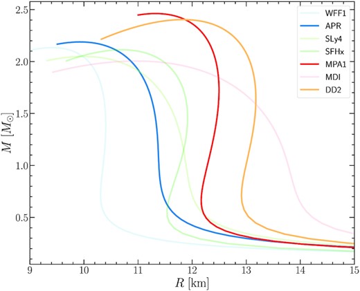
Gravitational mass M versus circumferential radius R of non-rotating models for different EOS.
Taking into account the above range of radii uncertainties, we selected three tabulated, zero-temperature, hadronic EOS that correspond to typical neutron star radii between 11 and 13 km. These are APR (Baym, Pethick & Sutherland 1971; Akmal, Pandharipande & Ravenhall 1998; Douchin & Haensel 2001), DD2 (Möller, Nix & Kratz 1997; Hempel & Schaffner-Bielich 2010; Typel et al. 2010) and MPA1 (Müther, Prakash & Ainsworth 1987), shown with darker colours in Fig. 1. All three EOS satisfy the current constraints for the maximum neutron star mass (Demorest et al. 2010; Antoniadis et al. 2013; Cromartie et al. 2020) as well as the minimum radius constraint, when combining causality and GW170817, of R1.6 ≥ 10.68 km (Bauswein et al. 2017). EOS with strong phase transitions are not included in this study.
2.5 Construction of merger remnant sequences
Our aim is to construct sequences of equilibrium models that mimic characteristic properties of post-merger remnants and reach the threshold mass to prompt collapse.
We construct sequences of models of merger remnants with different combinations of {λ1, λ2} and with remnant masses of |$M_\text{tot} = \lbrace 2.2, 2.3, 2.4, 2.5, \dots \rbrace \, \mathrm{M}_\odot$|. We continue to larger values with a step of |$0.1 \, \mathrm{M}_\odot$| up to the maximum possible Mtot for which we can construct an equilibrium sequence for the particular rotation law and EOS. For each value of Mtot, we compute the corresponding RNS and MNS of a non-rotating star. From (8) we compute the corresponding angular momentum of the remnant. The detailed properties of the equilibrium models of merger remnant sequences are reported and discussed in detail in Section 3.
2.6 Constant angular momentum sequences and turning points
The dynamical instability to prompt collapse to a black hole is detected through numerical simulations or by finding the models for which the frequency of the fundamental quasi-radial mode vanishes. For uniform rotation, the dynamical instability limit for prompt collapse is very close to the secular instability limit and it occurs slightly earlier (see Friedman & Stergioulas 2013) for a detailed discussion). In the case of differential rotation, Weih, Most & Rezzolla (2018) demonstrated (through numerical simulations) that for particular choices of the KEH law the dynamical instability also sets in very close to the secular instability limit (the central density of dynamically unstable models was at most several per cent smaller than the central density at the turning points).
Given the above findings for uniformly rotating as well as differentially rotating models with the KEH law and since we do not yet have dynamical or perturbative calculations for models constructed with the Uryu + law, we adopt the line connecting the turning points of constant angular momentum sequences as a reasonably approximate indicator of dynamical instability.
3 MAIN RESULTS
3.1 Sequences of type C models and threshold mass to prompt collapse
Initially, we focus on two combinations of {λ1, λ2} that were shown (Iosif & Stergioulas 2021) to yield Type C solutions according to the classification of Ansorg et al. (2009). These are sequences along which the models transition continuously from quasi-spherical to quasi-toroidal configurations, as the polar to equatorial axial ratio rp/re is decreased. We find that setting parameters {λ1, λ2} equal to the pairs of values {2.0, 0.5} and {1.5, 0.5}, continues to result in Type C solutions for the tabulated EOS we examined, as was the case for the N = 1 polytropes in Iosif & Stergioulas (2021).
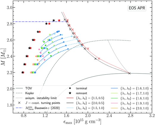
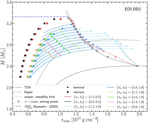
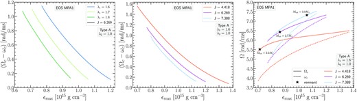
As can be seen in Fig. 2 for the APR EOS, the J-constant curves for both of these rotation laws are overlapping and the turning points we locate are quite close as well. This is to be expected, as these two particular rotation laws correspond to similar Ω(r) rotational profiles (fig. 8 Iosif & Stergioulas 2021). Asterisks in black and red denote the remnant models found for the respective Jmerger values predicted by the empirical relation (8). The gravitational masses of these configurations for the APR EOS start at |$2.2 \, \mathrm{M}_\odot$| for the least massive model and end at |$2.84 \, \mathrm{M}_\odot$| for the most massive model. The picture is similar for the other two EOS we consider, DD2 (see Fig. 3) and MPA1 (see Fig. 4). The only difference is that higher masses (as well as higher angular momentum values) are reached for the most massive remnant models at |$3.28 \, \mathrm{M}_\odot$| for DD2 and at |$3.2 \, \mathrm{M}_\odot$| for MPA1.
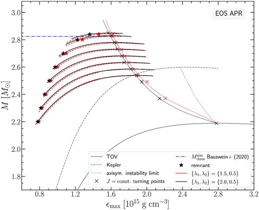
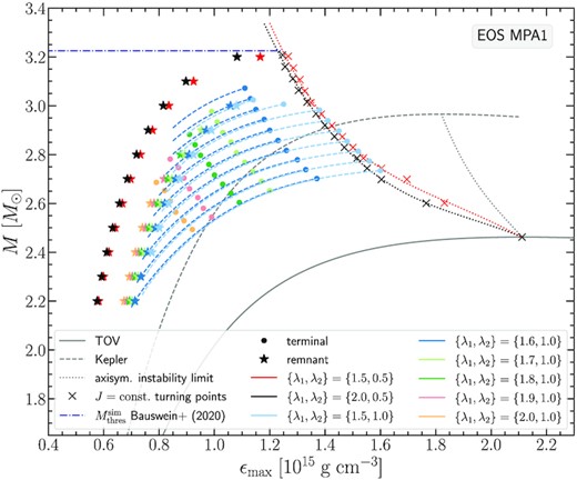
Gravitational mass M versus maximum energy density ϵmax for the APR EOS. Two choices of rotation law parameters yielding Type C solutions are shown. The non-rotating (TOV) sequence (grey solid line), the mass-shedding (Kepler) limit for uniform rotation (grey dashed line), and the axisymmetric instability limit for uniform rotation (grey dotted line) are shown as reference.
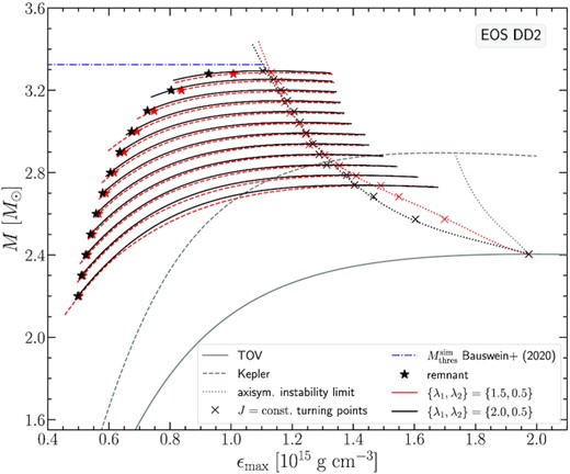
Same as Fig. 2 for the DD2 EOS.
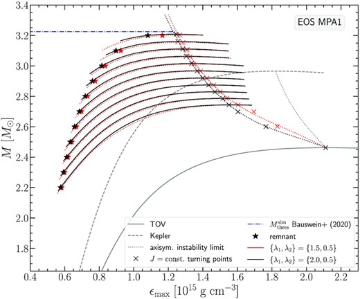
Same as Fig. 2 for the MPA1 EOS.
Qualitatively, the remnant sequence rises to larger masses at an almost constant (steep) slope that after a point abruptly diminishes, allowing the remnant sequence to intersect with the turning point line. As in Bauswein & Stergioulas (2017), we find that this intersection is related to the threshold mass for prompt collapse, |$M_\text{thres}^\text{sim}$| (as determined by numerical simulations in Bauswein et al. 2020). This mass is indicated by a blue horizontal dash-dotted line in Figs 2, 3, and 4. The intersection can also be determined in Figs 5, 6, and 7, which show the angular momentum J as a function of the gravitational mass M of the remnant sequence (blue line) and the line connecting the turning points of J-constant sequences for {λ1, λ2} = {2.0, 0.5} (black line) and {λ1, λ2} = {1.5, 0.5} (red line), for the three EOS. Note that the data for the remnant sequences in Figs 5, 6, and 7, as obtained from the empirical relation (8), form a straight line, in agreement with the form of the original empirical relation (7).

Angular momentum J versus gravitational mass M for the APR EOS. The intersection of the remnants’ and the turning points’ fitted lines determines the threshold mass to collapse calculated from our equilibrium models, |$M_\mathrm{thres}^\mathrm{eq}$|.
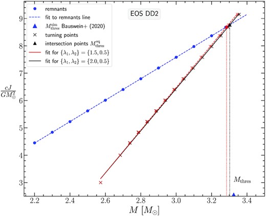
Same as Fig. 5 for the DD2 EOS.
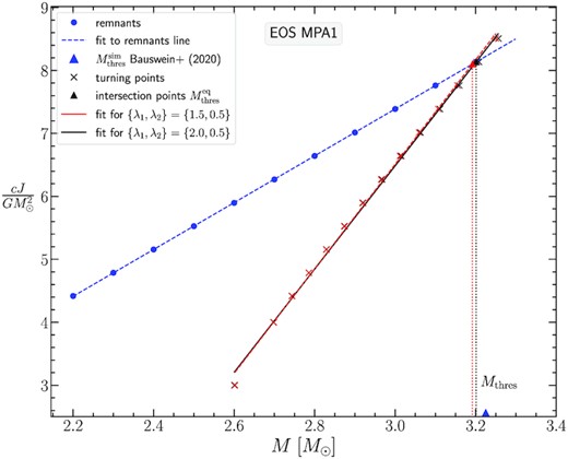
Same as Fig. 5 for the MPA1 EOS.
Coefficients of the linear fits J = aM − b and their respective errors that determine the intersection of the remnants sequence and the turning points line for each EOS (Figs 5, 6, and 7). The abbreviations RL, TP20, and TP15 stand for ‘remnant line’ and ‘turning point line’ with {λ1, λ2} = {2.0, 0.5} and {λ1, λ2} = {1.5, 0.5}, respectively. The errors in the coefficients of the linear fits, δa and δb, are calculated with the standard formulas of simple linear regression and correspond to uncertainties at the 1σ level.
| EOS | line | a | b | δa | δb |
|---|---|---|---|---|---|
| APR | RL | 3.3562 | 3.0453 | 0.0027 | 0.0069 |
| TP20 | 7.1189 | 13.7739 | 0.0823 | 0.2220 | |
| TP15 | 7.2199 | 14.0254 | 0.0827 | 0.2209 | |
| DD2 | RL | 3.9190 | 4.1758 | 0.0022 | 0.0062 |
| TP20 | 7.7087 | 16.6908 | 0.0523 | 0.1580 | |
| TP15 | 7.8003 | 16.9247 | 0.0530 | 0.1597 | |
| MPA1 | RL | 3.7183 | 3.7673 | 0.0029 | 0.0079 |
| TP20 | 8.2014 | 18.1185 | 0.1116 | 0.3294 | |
| TP15 | 8.3019 | 18.3962 | 0.1103 | 0.3253 |
Comparison of the threshold mass deduced from equilibrium models |$M_\text{thres}^\text{eq}$| with the respective quantity |$M_\text{thres}^\text{sim}$| from the numerical simulations of Bauswein et al. (2020). The angular momentum value we find at the intersection point, |$J_\text{thres}^\text{eq}$|, is also reported. The last column lists the absolute value of the relative difference δMthres calculated via (11).
| EOS | |$M_\text{thres}^\text{eq}$| | |$J_\text{thres}^\text{eq}$| | |$M_\text{thres}^\text{sim}$| | δMthres |
|---|---|---|---|---|
| {λ1, λ2} | (|$\, \mathrm{M}_\odot $|) | (|$\frac{G M_{\odot }^2}{c} $|) | (|$\, \mathrm{M}_\odot $|) | (per cent) |
| APR | – | – | 2.825 | – |
| {2.0, 0.5} | 2.851 | 6.524 | – | 0.92 |
| {1.5, 0.5} | 2.842 | 6.492 | – | 0.60 |
| DD2 | – | – | 3.325 | – |
| {2.0, 0.5} | 3.302 | 8.766 | – | 0.69 |
| {1.5, 0.5} | 3.285 | 8.697 | – | 1.20 |
| MPA1 | – | – | 3.225 | – |
| {2.0, 0.5} | 3.201 | 8.136 | – | 0.74 |
| {1.5, 0.5} | 3.192 | 8.100 | – | 1.02 |
Also, the agreement at the level of 1 per cent between our current models and numerical simulations is a significant improvement with respect to the agreement at the level of 3 per cent – 7 per cent in Bauswein & Stergioulas (2017), where a particular 3-parameter piecewise KEH-type rotation law was used. This is achieved without a direct reconstruction of particular merger remnants (i.e. without trying to match all properties of a remnant, as extracted from a numerical simulation), but using equilibrium models for particular {λ1, λ2} values, in conjunction with the empirical relation for the angular momentum at merger.
The above findings indicate that the Uryu + law is not simply qualitatively appropriate for merger remnants, in the sense that it allows for the maximum angular velocity to appear off-centre, but it can also yield precise numerical results, at least for certain properties of the remnants.
3.2 Domain of type A solutions
Merger remnants that do not collapse promptly, can evolve towards nearly axisymmetric, quasi-stationary configurations (at least before a possible delayed collapse sets in) that can be approximated with suitable equilibrium models. This involves Type A solutions,2 i.e. sequences of models that remain quasi-spherical (the maximum density is always at the centre) as the axial ratio rp/re is decreased (i.e. the rotation rate increases) until the mass-shedding limit is reached.
In our recent work Iosif & Stergioulas (2021), we found that the Uryu + rotation law with {λ1, λ2} = {2.0, 1.0} and with {λ1, λ2} = {1.5, 1.0} yields Type A solutions for the N = 1 polytropic EOS. In addition, we highlighted the fact that according to recent numerical simulations (Hanauske et al. 2017; De Pietri et al. 2020), a value of λ2 = 1 seems to be favoured over λ2 = 0.5, for the case of compact remnants from BNS mergers, while λ1 ranges between 1.7 and 1.9 for realistic EOS. We therefore probe in more detail models with this range of parameters. To that end, we set the value of λ2 to 1.0 and explore the range λ1 ∈ [1.5, 2.0] with a step of 0.1.
A vertical ‘scan’ of the mass versus ϵmax parameter space for specific Type A {λ1, λ2} pairs (fixing the value of the maximum energy density and gradually decreasing the axial ratio rp/re), revealed that these sequences reached a point, after which it was not possible to further construct equilibrium solutions as the maximum density was increased. This behaviour is much more stark for the case of {λ1, λ2} = {2.0, 1.0} than for {λ1, λ2} = {1.5, 1.0}. We note that the terminal models encountered for each choice of {λ1, λ2} pairs are not close to mass-shedding. For the highest {λ1, λ2} = {2.0, 1.0}, the Ωe/ΩK ratio of the terminal models ranges between 0.6 and 0.7 as the angular momentum increases, whereas for {λ1, λ2} = {1.5, 1.0} it ranges between 0.6 and 0.8. However, the maximum density remained at the centre of the configuration even at the highest rotation rates that were achieved and we classify these models as Type A.
Fig. 8 displays the six Type A remnant sequences corresponding to the six {λ1, λ2} pairs that we investigated3 for the APR EOS. Remnant models are shown as asterisks (different colours correspond to different {λ1, λ2} values). The terminal models along each J-constant sequence for each {λ1, λ2} pair are shown as dots of matching colour. We find that the choice of λ1 = 1.6 allows for the most massive Type A remnant model for this EOS, with a gravitational mass of |$M_\text{tot}=2.7 \, \mathrm{M}_\odot$|.
Gravitational mass M versus maximum energy density ϵmax for the APR EOS. Six choices of rotation law parameters yielding Type A solutions are presented (λ1 varies from 1.5 to 2 while λ2 is held fixed and equal to 1). The non-rotating (TOV) sequence (grey solid line), the mass-shedding (Kepler) limit for uniform rotation (grey dashed line), and the axisymmetric instability limit for uniform rotation (grey dotted line), together with the data corresponding to Type C solutions are shown as reference.
For the {λ1, λ2} = {1.5, 1.0} and {λ1, λ2} = {1.6, 1.0} cases, we explicitly show the constant angular momentum sequences (as light blue and dark blue dashed lines, respectively). We note that the {λ1, λ2} = {1.6, 1.0} J-constant lines in Fig. 8 nearly merge into those of {λ1, λ2} = {1.5, 1.0} as the maximum density increases. J-constant lines constructed with other pairs of {λ1, λ2} also tend to merge with those of {λ1, λ2} = {1.5, 1.0}, but for clarity, we omit the J-constant lines for λ1 = {1.7, 1.8, 1.9, 2.0} in Fig. 8. Moreover, as a rule of thumb the J-constant lines for {λ1, λ2} = {1.5, 1.0} reach higher maximum densities than the J-constant lines for {λ1, λ2} = {1.6, 1.0}. Note though, that for the highest J-constant sequence for the APR and DD2 EOS (Figs 8 and 9 respectively), this trend is reversed, i.e. it is the highest J-constant line for {λ1, λ2} = {1.6, 1.0} that actually reaches higher maximum densities. In our investigation of this behaviour, we found that an increasingly smaller step size in axial ratio was required (reaching as low as 10−4) to locate equilibrium solutions for {λ1, λ2} = {1.5, 1.0} (which yields the weakest differential rotation we consider) in the parameter space of increasing energy density values and high angular momentum values. This effect is indicating numerical stiffness. However, one would have to perform similar trials with other equilibrium codes to clarify whether this issue: (i) has some physical origin (e.g. it could be possible that weaker differential rotation cannot produce high enough angular velocities to accommodate arbitrarily high angular momentum values), (ii) or if it is due to numerical stiffness of the problem, (iii) or if it is due to the existence of different types of differentially rotating solutions that have the same central density and axial ratio.4
Same as Fig. 8 for the DD2 EOS.
Gathering all the evidence, some interesting observations can be made in connection to earlier works in the literature, where the KEH rotation law was used. First of all, we note that Type C remnant models are able to reach higher masses than Type A models, in agreement with findings in Gondek-Rosińska et al. (2017), Studzińska et al. (2016), Espino & Paschalidis (2019) for the KEH rotation law. Concerning the terminal models encountered for the Type A J-constant sequences, they can be interpreted as a confirmation that the domain of Type A solutions shrinks for higher densities and stronger differential rotation. Specifically, with stronger differential rotation we do not find Type A solutions above a certain maximum energy density, whereas we can still find Type C solutions5 (or Type A solutions with a weak differential rotation).
The above property of differentially rotating models was highlighted for the KEH rotation law in Studzińska et al. (2016), Gondek-Rosińska et al. (2017) for polytropes, Espino & Paschalidis (2019) for realistic EOS and Szkudlarek et al. (2019) for strange quark stars. From our findings for the Uryu + rotation law, it seems that the different types of solutions are not tied to the particular KEH rotation law (for which they were originally discovered), but appear also for other, more general rotation laws, such as the one by Uryū et al. considered here.
Figs 9 and 10 show the same investigation of Type A models as in Fig. 8, but for the EOS DD2 and MPA1. We note that also for these EOS, the choice of λ1 = 1.6 allows for the construction of the most massive Type A remnant model and also for a full remnant sequence (i.e. starting from the lowest remnant mass of |$M_\text{tot}=2.2 \, \mathrm{M}_\odot$| we consider). Within the parameter range that we investigated, the highest mass Type A remnant model reached with EOS DD2 was |$3.1 \, \mathrm{M}_\odot$|, while for EOS MPA1 it was |$3 \, \mathrm{M}_\odot$|.
Same as Fig. 8 for the MPA1 EOS.
In Iosif & Stergioulas (2021, fig. 8) we showed that for {λ1, λ2} = {1.5, 1.0} the differential rotation is quite weak, compared to other values of λ1 in the range we consider here. For the stiffest EOS we consider (DD2) this leads to Type A models for which we can find turning points along the J-constant sequences (light blue dotted curve in Fig. 9). Moreover, these turning points are close to the axisymmetric instability limit for uniform rotation.
3.3 Frame dragging contribution to rotation
Figs 11, 12, and 13 show the angular velocity Ω(rc) rotational profiles versus the circumferential radial coordinate rc at the equatorial plane, for the three EOS under study, APR, DD2, and MPA1. For each EOS, a triplet of panels is shown, with each left-hand panel corresponding to rotation laws {λ1, λ2} = {2.0, 0.5}, each middle panel to {λ1, λ2} = {1.5, 0.5}, and each right-hand panel to {λ1, λ2} = {1.6, 1.0}. Every individual panel shows Ω(rc), as well as the frame dragging angular velocity ω(rc) for the most massive, the least massive and for an intermediate mass remnant model constructed with the particular choice of parameters {λ1, λ2}. A common finding shared among the three EOS explored is that models with {λ1, λ2} = {2.0, 0.5} reach the highest angular velocity compared to the other two options and models with {λ1, λ2} = {1.6, 1.0} reach the smallest angular velocity peaks in their profile. This is in agreement with corresponding rotational profiles for these parameter values for polytropic equilibrium models with N = 1 (fig. 8 Iosif & Stergioulas 2021).
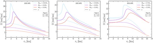
Angular velocity profiles Ω versus the circumferential radial coordinate rc, in the equatorial plane for the APR EOS. Left-hand panel: Type C models with {λ1, λ2} = {2.0, 0.5}. Middle panel: Type C models with {λ1, λ2} = {1.5, 0.5}. Right-hand panel: Type A models with {λ1, λ2} = {1.6, 1.0}. In each panel the profiles for the most massive, the least massive, and an intermediate mass remnant model are shown. The dashed lines correspond to the frame dragging angular velocity ω(rc) in the equatorial plane for each different model. For the most massive Type A model, we observe that Ω ≃ ω in the core, as has been reported in BNS merger simulations.
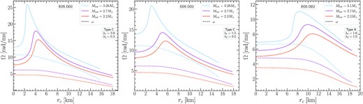
Same as Fig. 11 for the DD2 EOS.
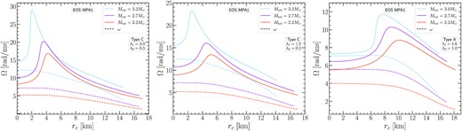
Same as Fig. 11 for the MPA1 EOS.
Examining Type A remnants, we observe that for the most massive models the central part of the configuration (i.e. approximately up to |$r_c \sim 5 \, \text{km}$|) rotates slowly compared to the rest of the configuration. However, this rotation rate is mostly due to the contribution of the frame dragging ω, which means that with respect to a ZAMO this part of the model is almost non-rotating. To our knowledge, this is the first time that a differential rotation law has been shown to reproduce this feature, already known from numerical simulations: similar rotation profiles have been presented and analysed in Kastaun & Galeazzi (2015), Endrizzi et al. (2016), Kastaun et al. (2016, 2017), Ciolfi et al. (2017).
Note that we did not observe the Ω ∼ ω behaviour near the centre of the star only for the most massive Type A models (i.e. the rightmost dark blue asterisks of the remnant sequences for {λ1, λ2} = {1.6, 1.0} in Figs 8, 9, and 10 corresponding to the light blue curves of the right-hand panels in Figs 11, 12, and 13 for each EOS considered). This feature also appears in less massive models that have higher central densities (i.e. models neighbouring the terminal models shown as dark blue dots for {λ1, λ2} = {1.6, 1.0} in Figs 8, 9, and 10). Specifically, for all the rotation law parameters yielding Type A configurations that we considered (i.e. the six {λ1, λ2} pairs with λ2 = 1.0 in Figs 8, 9, and 10), we found that ω approaches Ω as the maximum density increases along a J-constant sequence, until the Ω ∼ ω feature appears as we reach the terminal model. To clarify even further, we found that
along a J-constant sequence, the Ω ∼ ω behaviour appears at lower central densities as the strength of differential rotation is increased6 (see left-hand panel of Fig. 14).
for a specified strength of differential rotation (i.e. fixing the differential rotation law’s parameters at certain values), the Ω ∼ ω behaviour appears at lower central densities as the angular momentum J is increased (see middle panel of Fig. 14).
as the maximum energy density is increased along a J-constant sequence, the frame dragging at the centre ωc increases faster than the central angular velocity Ωc, thus giving rise to the Ω ∼ ω feature (see right-hand panel of Fig. 14).
Note that while Fig. 14 demonstrates the above for the MPA1 EOS, similar behaviour is observed for the other two EOS that we studied.
Investigation of the frame dragging contribution to rotation for the MPA1 EOS. Left-hand panel: Difference (Ωc − ωc) between the angular velocity and the frame dragging values at the centre of the configuration versus the maximum energy density. The solid lines correspond to J-constant sequences with J = 6.269, along which remnant models with |$M_\text{tot}=2.7 \, \mathrm{M}_\odot$| are constructed. The colours represent different options for λ1 yielding different strengths of differential rotation and are matching the colours of the respective options in Fig. 10 for ease of reference. Middle panel: Same quantities plotted as in the left-hand panel, but for a single strength of differential rotation {λ1, λ2} = {1.6, 1.0}. The solid lines are J-constant sequences corresponding to the most massive (|$M_\text{tot}=3.0 \, \mathrm{M}_\odot$|), least massive (|$M_\text{tot}=2.2 \, \mathrm{M}_\odot$|), and an intermediate mass |$M_\text{tot}=2.7 \, \mathrm{M}_\odot$| remnant model. Right-hand panel: Central angular velocity Ωc (solid lines) and frame dragging at the centre ωc (dashed lines) versus the maximum energy density for {λ1, λ2} = {1.6, 1.0}. The different colours correspond to the same J-constant sequences as in the middle panel. The asterisks represent the respective remnant models. The colours selected in the middle and right-hand panels match those of the right-hand panel of Fig. 13 for ease of reference.
3.4 Ω(F) profiles
Figs 15, 16, and 17 follow the same organization as corresponding figures for the rotation profiles Ω(rc) and present the angular velocity Ω(F) profiles that define each rotation law. We find that for each choice of rotation law parameters (e.g. if one observes the left-hand panels of Figs 15, 16, and 17 ‘vertically’, etc.) the resulting Ω(F) profiles are qualitatively similar between the three EOS that we consider. This is in agreement with analogous behaviour of the corresponding Ω(rc) profiles in Figs 11, 12, and 13.
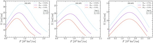
Angular velocity profiles Ω versus the gravitationally redshifted angular momentum per unit rest mass and enthalpy F, in the equatorial plane for the APR EOS. Left-hand panel: Type C models with {λ1, λ2} = {2.0, 0.5}. Middle panel: Type C models with {λ1, λ2} = {1.5, 0.5}. Right-hand panel: Type A models with {λ1, λ2} = {1.6, 1.0}. In each panel the profiles for the most massive, the least massive, and an intermediate mass remnant model are shown.
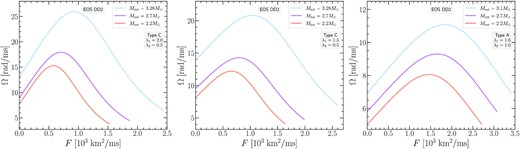
Same as Fig. 15 for the DD2 EOS.
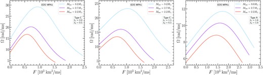
Same as Fig. 15 for the MPA1 EOS.
Note that in all cases, the inverse profile, F(Ω), would not be a one-to-one function. In the case of the KEH rotation law, one can simply integrate F(Ω) in the equation of hydrostationary equilibrium. However, for the Uryu + rotation law, one needs to express the equation of stationary equilibrium in terms of an integral Ω(F) (see Iosif & Stergioulas (2021) for details).
3.5 Structure of the remnants: surface and density distribution
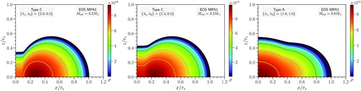
Stellar surfaces in the x − z plane (with x and z normalized with the equatorial coordinate radius re) for the most massive, least massive, and an intermediate mass remnant model are shown in Figs 18, 19, and 20, for the three EOS employed and for three different choices of parameters {λ1, λ2} (similar to the corresponding figures of the rotation profiles). We note that for tabulated EOS we always have a finite minimum pressure value Pmin at the minimum density ρmin. For the three EOS employed, the range of ρmin is sub-grid varying from |$\sim 8 \, \mathrm{g \, cm^{-3}}$| to |$\sim 10^3 \, \mathrm{g \, cm^{-3}}$|, i.e. so small that not a single grid point is removed from the model. Furthermore, since the rns code constructs numerical tables in log enthalpy, a very small enthalpy value Hmin (of the order of 10−16) is used in the tabulated EOS files. Then, the stellar surface is defined as the location where the pressure P = Pmin and the enthalpy H = Hmin. Interpolating the model’s enthalpy by demanding that its value matches Hmin allows us to pinpoint the surface’s location. In addition, Figs 21, 22, and 23 display the 2D rest-mass density distributions for the most massive models in the meridional plane.
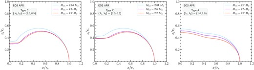
Stellar surfaces for the APR EOS. Left-hand panel: Type C models with {λ1, λ2} = {2.0, 0.5}. Middle panel: Type C models with {λ1, λ2} = {1.5, 0.5}. Right-hand panel: Type A models with {λ1, λ2} = {1.6, 1.0}. In each panel the surfaces of the most massive, the least massive, and an intermediate mass remnant model are shown.
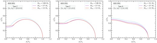
Same as Fig. 18 for the DD2 EOS.
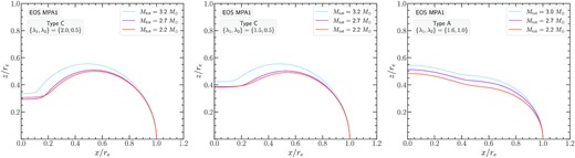
Same as Fig. 18 for the MPA1 EOS.
![2D rest mass density distribution $\rho \, [\mathrm{g \, cm^{-3}}]$ of the most massive remnant models for the APR EOS. Left-hand panel: Type C model with {λ1, λ2} = {2.0, 0.5}. Middle panel: Type C model with {λ1, λ2} = {1.5, 0.5}. Right-hand panel: Type A model with {λ1, λ2} = {1.6, 1.0}.](https://oup.silverchair-cdn.com/oup/backfile/Content_public/Journal/mnras/510/2/10.1093_mnras_stab3565/1/m_stab3565fig21.jpeg?Expires=1750041027&Signature=3Iof2u4bgBq62wic3yuWPf6sMqNyy59eAJ3Yx88KYi2y3sGVxv6uCjuWYiBF3-AjxccfI581VGJfeT9dp~NhiBppWmavh8DQUHqJbEBT8km1zcfEKHMmdr14CHLUkT6FL-sE9EuT4qnhw0mnnysQa1k9ZyQZIRWbaSTy0dLc1UVzplC41I6JUbzD9tKOTs~MLNTnXYSSXZZiB~S6bqlfXYxox4a6EI9KJgzln977iATZj2I3NYp4ZV6XnoDqEs-goMDxsitrE6FEVdAHtoexH8pTPYea-FaM5Q~DV0TUF374J33D5Qm70NkJyK8WuryJtqmvbZhH7jDiTBN92VS9XA__&Key-Pair-Id=APKAIE5G5CRDK6RD3PGA)
2D rest mass density distribution |$\rho \, [\mathrm{g \, cm^{-3}}]$| of the most massive remnant models for the APR EOS. Left-hand panel: Type C model with {λ1, λ2} = {2.0, 0.5}. Middle panel: Type C model with {λ1, λ2} = {1.5, 0.5}. Right-hand panel: Type A model with {λ1, λ2} = {1.6, 1.0}.
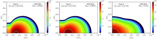
Same as Fig. 21 for the DD2 EOS.
Same as Fig. 21 for the MPA1 EOS.
Note that the surfaces and meridional density profiles are qualitatively similar for the Type C solutions obtained with {λ1, λ2} = {2.0, 0.5} and {λ1, λ2} = {1.5, 0.5}. Both choices lead to a quasi-toroidal surface shape, typical for Type C solutions. For {λ1, λ2} = {2.0, 0.5}, we observe a stronger deformation close to the rotation axis than for {λ1, λ2} = {1.5, 0.5}, which is explained by the stronger differential rotation.
For the Type A solutions obtained with {λ1, λ2} = {1.6, 1.0}, the surfaces of all models (most massive to least massive) are quite similar to each other (when coordinates are scaled by re). Even though the remnant models have significant oblateness, they still retain their quasi-spherical shape (the central density is also the maximum density). It is interesting to note that for these selected Type A remnants, the axial ratio rp/re ranges between ∼0.47 and 0.54, whereas for the Type C remnants the corresponding range is considerably lower at ∼0.3−0.42.
Recently, Kastaun et al. (2016) introduced a new measure that replaces density profiles, mass, and compactness in a way that can be used unambiguously for rapidly and differentially rotating merger remnants, without a clearly defined surface. Therefore, we stress that the profiles presented here serve simply as an indication about the different configurations possible for the different cold EOS employed and for the {λ1, λ2} options we considered. In a realistic remnant with a hot envelope and mass-shedding, the density distribution would not terminate at the same radius as in our models and one would need to define an approximate surface shape, based e.g. on the location where the density drops to a certain fraction of the maximum density.
3.6 Mass versus equatorial radius
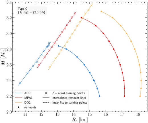
Having presented the main characteristics of our models in the previous subsections, we further analyse our findings by constructing M(Re) plots (i.e. gravitational mass versus equatorial circumferential radius) for the remnant models. We focus on the choice {λ1, λ2} = {2.0, 0.5} that represents the strongest differential rotation we consider, but note that a similar picture holds for the case {λ1, λ2} = {1.5, 0.5}.
Figs 24, 25, and 26 show M(Re) for the EOS APR, DD2, and MPA1 respectively. In each of these figures, remnant sequences are shown as dots (denoting the equilibrium models), connected by solid interpolated lines. The dotted lines represent J-constant sequences, turning points are marked by crosses and a linear fit (dashed line) approximates the turning point sequence. The annotation in these figures means that while the empirical relation (8) by Lucca et al. (2021) provides a predicted Jmerger value for a desired target value Mtot, the intersection of the remnant sequence and the turning point sequence has already taken place. Therefore, the target Mtot model for the specific Jmerger value predicted by (8), does not exist, since it would exceed the value of Mthres.
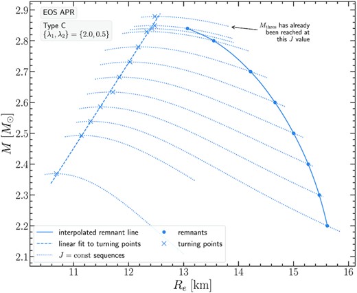
Gravitational mass M versus equatorial circumferential radius Re for models constructed with the Uryu + rotation law, using {λ1, λ2} = {2.0, 0.5}, for the APR EOS. Each dotted line is a J-constant sequence and a cross indicates the turning point model. The dashed line is a linear fit through the turning point models. The filled circles represent the sequence of remnant models.
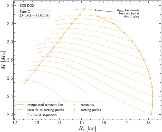
Same as Fig. 24 for the DD2 EOS.
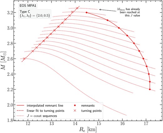
Same as Fig. 24 for the MPA1 EOS.
Coefficients of the linear fits M = a1Re − b1 and their respective errors, for the turning point sequences with {λ1, λ2} = {2.0, 0.5} of each EOS (Figs 24, 25, and 26). The errors in the coefficients of the linear fits, δa1 and δb1, are calculated with the standard formulas of simple linear regression and correspond to uncertainties at the 1σ level.
| EOS | a1 | b1 | δa1 | δb1 |
|---|---|---|---|---|
| APR | 0.2769 | 0.5936 | 0.0048 | 0.0574 |
| DD2 | 0.3077 | 1.2876 | 0.0040 | 0.0564 |
| MPA1 | 0.2969 | 0.9268 | 0.0029 | 0.0382 |
| EOS | a1 | b1 | δa1 | δb1 |
|---|---|---|---|---|
| APR | 0.2769 | 0.5936 | 0.0048 | 0.0574 |
| DD2 | 0.3077 | 1.2876 | 0.0040 | 0.0564 |
| MPA1 | 0.2969 | 0.9268 | 0.0029 | 0.0382 |
Collecting data from all EOS in a single M(Re) plot, Fig. 27, one could extrapolate the remnant sequences so that they intersect with the turning point sequences and obtain the intersection (Mthres, Re − thres). We note that the Mthres values determined in this way are in good agreement with those reported in Table 2. Still, we regard the values in Table 2 as better estimates for |$M_\text{thres}^\text{eq}$|, since they involve bulk quantities of the star, such as the angular momentum J and the mass M, with direct input from numerical simulations, via (8), to determine J. Moreover, the precise determination of Re − thres, in actual remnants is affected by the thermal properties of low-density material and one needs to resort to a particular definition, based on an isodensity surface, where the density has become a certain small fraction of the maximum density. The notion of a ‘bulk’ region and the relative measure introduced in Kastaun et al. (2016) is relevant in this respect.
Same as Fig. 24, showing collectively remnants and turning points for all EOS considered.
3.7 Mass versus equatorial compactness and a criterion for prompt collapse
The almost identical slope of the turning point lines in the M(Re) plot of Fig. 27, implies that the threshold mass to collapse will be attained at about the same value of the ratio M/Re, for all three EOS considered. In correspondence to the usual definition of the compactness of a non-rotating star C = M/R, we define the ratio Ce = M/Re as the equatorial compactness.
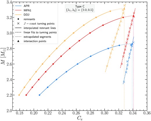
Gravitational mass M versus equatorial compactness Ce for all EOS considered for the Type C models with {λ1, λ2} = {2.0, 0.5}.
Coefficients of the linear fits M = a2C − b2 and their respective errors, for the turning point sequences with {λ1, λ2} = {2.0, 0.5} of each EOS (Fig. 28). The errors in the coefficients of the linear fits, δa2 and δb2, are calculated with the standard formulas of simple linear regression and correspond to uncertainties at the 1σ level. Values for Ce − thres at the intersection points are also listed, together with the corresponding values for |$C_\text{max}^{\rm TOV}$| of the maximum mass TOV model for each EOS.
| EOS | a2 | b2 | δa2 | δb2 | Ce − thres | |$C_\text{max}^{\rm TOV}$| |
|---|---|---|---|---|---|---|
| APR | 40.6218 | 10.9095 | 2.8194 | 0.9435 | 0.339 | 0.326 |
| DD2 | 30.4530 | 6.6678 | 0.8999 | 0.2854 | 0.328 | 0.300 |
| MPA1 | 36.3972 | 9.1811 | 0.7741 | 0.2579 | 0.341 | 0.321 |
| EOS | a2 | b2 | δa2 | δb2 | Ce − thres | |$C_\text{max}^{\rm TOV}$| |
|---|---|---|---|---|---|---|
| APR | 40.6218 | 10.9095 | 2.8194 | 0.9435 | 0.339 | 0.326 |
| DD2 | 30.4530 | 6.6678 | 0.8999 | 0.2854 | 0.328 | 0.300 |
| MPA1 | 36.3972 | 9.1811 | 0.7741 | 0.2579 | 0.341 | 0.321 |
Physical quantities for equilibrium remnant models constructed with the APR EOS and different choices of rotation law parameters. The columns show the polar to equatorial axial ratio rp/re, the central energy density ϵc, the maximum energy density ϵmax, the gravitational mass M, the rest mass M0, the angular momentum J, the ratio of the rotational kinetic energy T over the absolute value of the gravitational binding energy |W|, the angular velocity at the rotation axis Ωc, the maximum value of angular velocity Ωmax, the angular velocity at the equator Ωe, the angular velocity of a free particle in circular orbit at the equator ΩK, the circumferential radius Re, the coordinate radius re at the equator, and the 3D general relativistic virial index GRV3.
| rp/re | ϵc(× 1015) | ϵmax(× 1015) | M | M0 | J | T/|W| | Ωc | Ωmax | Ωe | ΩK | Re | re | GRV3 |
|---|---|---|---|---|---|---|---|---|---|---|---|---|---|
| {λ1, λ2} | |$(\mathrm{g \, cm^{-3}})$| | |$(\mathrm{g \, cm^{-3}})$| | (M⊙) | (M⊙) | |$(\frac{G M_{\odot }^2}{c})$| | (rad ms−1) | (rad ms−1) | (rad ms−1) | (rad ms−1) | (km) | (km) | (× 10−5) | |
| {2.0, 0.5} | |||||||||||||
| 0.2981 | 0.543 | 0.7788 | 2.20 | 2.4297 | 4.3365 | 0.2253 | 9.9765 | 19.9530 | 4.9882 | 9.1037 | 15.6150 | 11.8159 | 7.6519 |
| 0.2952 | 0.563 | 0.8138 | 2.30 | 2.5558 | 4.6733 | 0.2258 | 10.4436 | 20.8873 | 5.2218 | 9.4001 | 15.4686 | 11.4730 | 6.4827 |
| 0.2950 | 0.592 | 0.8556 | 2.40 | 2.6847 | 5.0105 | 0.2257 | 10.9829 | 21.9658 | 5.4914 | 9.7420 | 15.2677 | 11.0720 | 7.6786 |
| 0.2976 | 0.632 | 0.9074 | 2.50 | 2.8175 | 5.3469 | 0.2250 | 11.6224 | 23.2451 | 5.8112 | 10.1461 | 15.0024 | 10.6012 | 6.8382 |
| 0.3027 | 0.685 | 0.9736 | 2.60 | 2.9540 | 5.6820 | 0.2239 | 12.4015 | 24.8030 | 6.2007 | 10.6314 | 14.6637 | 10.0506 | 6.3562 |
| 0.3100 | 0.758 | 1.0659 | 2.70 | 3.0956 | 6.0176 | 0.2223 | 13.4186 | 26.8376 | 6.7093 | 11.2489 | 14.2197 | 9.3826 | 7.4427 |
| 0.3204 | 0.879 | 1.2256 | 2.80 | 3.2440 | 6.3517 | 0.2203 | 15.0118 | 30.0244 | 7.5059 | 12.1789 | 13.5483 | 8.4607 | 8.7865 |
| 0.3261 | 0.976 | 1.3619 | 2.84 | 3.3058 | 6.4839 | 0.2194 | 16.2264 | 32.4557 | 8.1132 | 12.8548 | 13.0703 | 7.8583 | 7.9165 |
| {1.5, 0.5} | |||||||||||||
| 0.3806 | 0.720 | 0.7911 | 2.20 | 2.4383 | 4.3365 | 0.2229 | 10.6528 | 15.9793 | 5.3264 | 9.2112 | 15.4348 | 11.6363 | 7.8407 |
| 0.3795 | 0.748 | 0.8280 | 2.30 | 2.5648 | 4.6734 | 0.2233 | 11.1264 | 16.6896 | 5.5632 | 9.5197 | 15.2823 | 11.2862 | 6.3160 |
| 0.3807 | 0.784 | 0.8722 | 2.40 | 2.6946 | 5.0105 | 0.2231 | 11.6700 | 17.5050 | 5.8350 | 9.8752 | 15.0766 | 10.8789 | 7.9935 |
| 0.3843 | 0.831 | 0.9276 | 2.50 | 2.8286 | 5.3469 | 0.2221 | 12.3134 | 18.4701 | 6.1567 | 10.2962 | 14.8070 | 10.4015 | 7.1972 |
| 0.3897 | 0.892 | 0.9985 | 2.60 | 2.9658 | 5.6820 | 0.2206 | 13.0935 | 19.6402 | 6.5467 | 10.7975 | 14.4685 | 9.8486 | 7.1570 |
| 0.3970 | 0.978 | 1.0986 | 2.70 | 3.1081 | 6.0175 | 0.2187 | 14.1200 | 21.1800 | 7.0600 | 11.4392 | 14.0226 | 9.1754 | 7.4033 |
| 0.4067 | 1.130 | 1.2790 | 2.80 | 3.2566 | 6.3517 | 0.2165 | 15.7837 | 23.6757 | 7.8919 | 12.4311 | 13.3304 | 8.2262 | 8.4743 |
| 0.4119 | 1.281 | 1.4642 | 2.84 | 3.3179 | 6.4839 | 0.2156 | 17.2826 | 25.9241 | 8.6413 | 13.2718 | 12.7567 | 7.5147 | 9.6980 |
| {1.6, 1.0} | |||||||||||||
| 0.4669 | 1.0128 | 1.0128 | 2.20 | 2.4567 | 4.3365 | 0.2052 | 6.4676 | 10.3482 | 6.4676 | 7.9280 | 16.8809 | 13.1466 | 9.4359 |
| 0.4813 | 1.0583 | 1.0583 | 2.30 | 2.5862 | 4.6733 | 0.2056 | 6.7609 | 10.8175 | 6.7609 | 8.5470 | 16.2804 | 12.3306 | 9.2157 |
| 0.4930 | 1.1154 | 1.1154 | 2.40 | 2.7188 | 5.0105 | 0.2051 | 7.0683 | 11.3092 | 7.0683 | 9.1070 | 15.7973 | 11.6330 | 9.5772 |
| 0.5051 | 1.1883 | 1.1883 | 2.50 | 2.8551 | 5.3468 | 0.2038 | 7.4161 | 11.8658 | 7.4161 | 9.6956 | 15.3167 | 10.9335 | 9.8606 |
| 0.5185 | 1.2862 | 1.2862 | 2.60 | 2.9961 | 5.6820 | 0.2018 | 7.8342 | 12.5347 | 7.8342 | 10.3614 | 14.7943 | 10.1838 | 11.8614 |
| 0.5334 | 1.4320 | 1.4320 | 2.70 | 3.1421 | 6.0175 | 0.1996 | 8.3892 | 13.4227 | 8.3892 | 11.1812 | 14.1770 | 9.3242 | 12.3628 |
Physical quantities for equilibrium remnant models constructed with the DD2 EOS and different choices of rotation law parameters. The different quantities are defined as in Table 5.
| rp/re | ϵc(× 1015) | ϵmax(× 1015) | M | M0 | J | T/|W| | Ωc | Ωmax | Ωe | ΩK | Re | re | GRV3 |
|---|---|---|---|---|---|---|---|---|---|---|---|---|---|
| {λ1, λ2} | |$(\mathrm{g \, cm^{-3}})$| | |$(\mathrm{g \, cm^{-3}})$| | |$(\, \mathrm{M}_\odot)$| | |$(\, \mathrm{M}_\odot )$| | |$(\frac{G M_{\odot }^2}{c})$| | (rad ms−1) | (rad ms−1) | (rad ms−1) | (rad ms−1) | (km) | (km) | (× 10−5) | |
| {2.0, 0.5} | |||||||||||||
| 0.3208 | 0.3812 | 0.4983 | 2.20 | 2.4009 | 4.4513 | 0.2172 | 7.6442 | 15.2884 | 3.8221 | 7.3691 | 18.1234 | 14.3799 | 8.3706 |
| 0.3094 | 0.3789 | 0.5101 | 2.30 | 2.5198 | 4.8401 | 0.2198 | 7.8595 | 15.7190 | 3.9298 | 7.4853 | 18.1858 | 14.2529 | 6.9913 |
| 0.3015 | 0.3807 | 0.5240 | 2.40 | 2.6406 | 5.2273 | 0.2215 | 8.0980 | 16.1960 | 4.0490 | 7.6254 | 18.1922 | 14.0690 | 7.7354 |
| 0.2952 | 0.3847 | 0.5396 | 2.50 | 2.7630 | 5.6204 | 0.2228 | 8.3557 | 16.7114 | 4.1778 | 7.7787 | 18.1660 | 13.8509 | 10.1183 |
| 0.2921 | 0.3935 | 0.5581 | 2.60 | 2.8877 | 6.0109 | 0.2234 | 8.6459 | 17.2919 | 4.3230 | 7.9591 | 18.0857 | 13.5768 | 6.9961 |
| 0.2911 | 0.4060 | 0.5795 | 2.70 | 3.0146 | 6.4027 | 0.2236 | 8.9700 | 17.9401 | 4.4850 | 8.1617 | 17.9628 | 13.2582 | 6.9080 |
| 0.2922 | 0.4230 | 0.6051 | 2.80 | 3.1443 | 6.7954 | 0.2234 | 9.3389 | 18.6779 | 4.6694 | 8.3936 | 17.7916 | 12.8879 | 7.8284 |
| 0.2952 | 0.4447 | 0.6359 | 2.90 | 3.2768 | 7.1887 | 0.2229 | 9.7627 | 19.5254 | 4.8813 | 8.6588 | 17.5710 | 12.4645 | 6.3214 |
| 0.2999 | 0.4726 | 0.6745 | 3.00 | 3.4125 | 7.5817 | 0.2220 | 10.2658 | 20.5315 | 5.1329 | 8.9707 | 17.2880 | 11.9735 | 6.1169 |
| 0.3065 | 0.5100 | 0.7266 | 3.10 | 3.5524 | 7.9741 | 0.2209 | 10.8964 | 21.7932 | 5.4482 | 9.3560 | 16.9163 | 11.3854 | 7.7065 |
| 0.3145 | 0.5630 | 0.8044 | 3.20 | 3.6962 | 8.3673 | 0.2196 | 11.7581 | 23.5171 | 5.8791 | 9.8656 | 16.4095 | 10.6486 | 7.2057 |
| 0.3226 | 0.6410 | 0.9276 | 3.28 | 3.8156 | 8.6800 | 0.2188 | 12.9607 | 25.9233 | 6.4803 | 10.5450 | 15.7235 | 9.7506 | 7.2275 |
| {1.5, 0.5} | |||||||||||||
| 0.3962 | 0.4716 | 0.5025 | 2.20 | 2.4074 | 4.4513 | 0.2142 | 8.1481 | 12.2221 | 4.0740 | 7.4195 | 17.9799 | 14.2399 | 7.0193 |
| 0.3884 | 0.4773 | 0.5151 | 2.30 | 2.5270 | 4.8401 | 0.2171 | 8.3792 | 12.5687 | 4.1896 | 7.5467 | 18.0227 | 14.0929 | 8.6483 |
| 0.3833 | 0.4860 | 0.5299 | 2.40 | 2.6485 | 5.2272 | 0.2190 | 8.6292 | 12.9438 | 4.3146 | 7.6968 | 18.0142 | 13.8936 | 7.0557 |
| 0.3799 | 0.4970 | 0.5468 | 2.50 | 2.7723 | 5.6203 | 0.2203 | 8.9002 | 13.3503 | 4.4501 | 7.8635 | 17.9698 | 13.6556 | 8.5267 |
| 0.3784 | 0.5110 | 0.5663 | 2.60 | 2.8973 | 6.0109 | 0.2209 | 9.1956 | 13.7934 | 4.5978 | 8.0505 | 17.8832 | 13.3750 | 9.3444 |
| 0.3789 | 0.5290 | 0.5895 | 2.70 | 3.0256 | 6.4027 | 0.2210 | 9.5275 | 14.2913 | 4.7638 | 8.2655 | 17.7494 | 13.0433 | 6.7115 |
| 0.3808 | 0.5510 | 0.6168 | 2.80 | 3.1562 | 6.7955 | 0.2206 | 9.9002 | 14.8504 | 4.9501 | 8.5067 | 17.5734 | 12.6666 | 7.3657 |
| 0.3839 | 0.5778 | 0.6495 | 2.90 | 3.2889 | 7.1888 | 0.2199 | 10.3245 | 15.4868 | 5.1623 | 8.7788 | 17.3533 | 12.2428 | 7.5190 |
| 0.3887 | 0.6130 | 0.6916 | 3.00 | 3.4258 | 7.5817 | 0.2188 | 10.8354 | 16.2531 | 5.4177 | 9.1050 | 17.0641 | 11.7429 | 6.8216 |
| 0.3946 | 0.6600 | 0.7482 | 3.10 | 3.5656 | 7.9741 | 0.2176 | 11.4737 | 17.2106 | 5.7369 | 9.5030 | 16.6920 | 11.1526 | 7.5437 |
| 0.4020 | 0.7330 | 0.8376 | 3.20 | 3.7105 | 8.3673 | 0.2161 | 12.3874 | 18.5812 | 6.1937 | 10.0535 | 16.1580 | 10.3829 | 7.4784 |
| 0.4090 | 0.8670 | 1.0083 | 3.28 | 3.8301 | 8.6800 | 0.2155 | 13.8873 | 20.8311 | 6.9437 | 10.9019 | 15.3236 | 9.3187 | 8.2883 |
| {1.6, 1.0} | |||||||||||||
| 0.4828 | 0.6261 | 0.6261 | 2.20 | 2.4207 | 4.4513 | 0.1992 | 5.0343 | 8.0549 | 5.0343 | 6.5162 | 19.4227 | 15.7321 | 8.5887 |
| 0.4829 | 0.6451 | 0.6451 | 2.30 | 2.5421 | 4.8400 | 0.2019 | 5.1666 | 8.2666 | 5.1666 | 6.7141 | 19.3079 | 15.4256 | 9.8640 |
| 0.4854 | 0.6669 | 0.6670 | 2.40 | 2.6658 | 5.2273 | 0.2034 | 5.3104 | 8.4966 | 5.3104 | 6.9468 | 19.1243 | 15.0469 | 8.9839 |
| 0.4885 | 0.6916 | 0.6916 | 2.50 | 2.7912 | 5.6203 | 0.2045 | 5.4627 | 8.7404 | 5.4627 | 7.1879 | 18.9252 | 14.6504 | 10.0100 |
| 0.4933 | 0.7209 | 0.7209 | 2.60 | 2.9192 | 6.0109 | 0.2048 | 5.6300 | 9.0080 | 5.6300 | 7.4581 | 18.6776 | 14.2023 | 8.8487 |
| 0.4990 | 0.7556 | 0.7556 | 2.70 | 3.0495 | 6.4027 | 0.2045 | 5.8134 | 9.3014 | 5.8134 | 7.7484 | 18.4016 | 13.7228 | 9.1569 |
| 0.5058 | 0.7978 | 0.7978 | 2.80 | 3.1827 | 6.7953 | 0.2037 | 6.0192 | 9.6308 | 6.0192 | 8.0671 | 18.0894 | 13.2030 | 10.1405 |
| 0.5134 | 0.8510 | 0.8510 | 2.90 | 3.3189 | 7.1888 | 0.2026 | 6.2561 | 10.0098 | 6.2561 | 8.4222 | 17.7347 | 12.6358 | 9.5439 |
| 0.5222 | 0.9226 | 0.9226 | 3.00 | 3.4589 | 7.5818 | 0.2010 | 6.5434 | 10.4695 | 6.5434 | 8.8369 | 17.3132 | 11.9945 | 10.9882 |
| 0.5322 | 1.0304 | 1.0304 | 3.10 | 3.6029 | 7.9740 | 0.1992 | 6.9248 | 11.0797 | 6.9248 | 9.3564 | 16.7807 | 11.2302 | 11.8057 |
It is interesting that in simulations with the SFHo EOS by Kastaun & Ohme (2021) a ‘bulk’ compactness of 0.31 for the remnant 1ms before collapse is reported, with |$C_\text{max}^{\rm TOV}=0.295$| for the maximum mass TOV model for this specific EOS. In Kastaun et al. (2016) it was found that the core of the remnant has a mass profile that resembles that of a TOV solution, with similar findings echoed by Ciolfi et al. (2017). The latter study went on to suggest the conjecture that merger remnants that do not admit a TOV core equivalent8 promptly collapse to a black hole. It will be interesting to explore these prospects with equilibrium modelling in future work, now that we have provided proof of concept that the Uryu + law can capture the Ω ∼ ω feature in the core of remnants, as it has been observed in simulations. We note that the physical quantities of our remnant models are collectively reported in Tables 5, 6, and 7 for EOS APR, DD2, and MPA1.
4 DISCUSSION AND OUTLOOK
In this study, we followed up on our recent work (Iosif & Stergioulas 2021) and expanded our investigation of relativistic equilibrium models, using the 4-parameter differential rotation law of Uryū et al. (2017) and cold, tabulated EOS of high-density matter. We constructed sequences of merger remnants, taking advantage of empirical relations for the angular momentum at merger, derived through numerical simulations. Comparing the rotational profiles Ω(rc), the Ω(F) profiles, the stellar surfaces and the meridional rest mass density profiles of our remnant models between the three EOS we employed, we found that all respective profiles studied are qualitatively similar when the rotation law parameters are held fixed to different values. Furthermore, choices for the rotation law parameters that yield the same Type of solutions (i.e. either Type A or C) also show qualitative similarities in profiles even when varying the parameter λ1.
In addition, we constructed constant angular momentum sequences. From the intersection of the line connecting the turning points of J-constant sequences and the merger remnant sequence, we were able to reproduce the threshold mass to prompt collapse, Mthres with a relative difference of only |$\sim 1{{\ \rm per\ cent}}$|, compared to accurate binary neutron star merger simulations. We stress that this was achieved using the same rotation law, i.e. the same values for the rotation law parameters {λ1, λ2} for all three EOS used in this study.
Our investigation of the threshold mass to collapse, using equilibrium models, also points towards a possible connection between the equatorial compactness Ce = M/Re at the threshold and the maximum compactness of non-rotating models |$C_\text{max}^\text{TOV}$|. This lends support to the conjecture by Ciolfi et al. (2017), that merger remnants collapse if their relatively cold and slowly rotating inner region does not admit a stable TOV equivalent.
Another key prediction of binary neutron star merger simulations is a relatively slowly rotating inner region, where the angular velocity Ω (as measured by an observer at infinity) is mostly due to the frame dragging angular velocity ω. In our investigation of the parameter space of the Uryu + rotation law, we naturally find quasi-spherical (Type A) remnant models with this property. Both the density distribution and the angular velocity profile of these models have striking similarities with merger remnants produced in simulations (except for the low-density regions, since we neglect thermal effects).
In a forthcoming study, we plan to take the next step in this program and construct equilibrium models with finite-temperature EOS, using temperature and electron fraction profiles extracted from simulations of BNS mergers. This should allow us to isolate the effect of the thermal state of the remnant on the key properties that we discuss above. Based on Kaplan et al. (2014), Camelio et al. (2019), Camelio et al. (2021), Chakravarti & Andersson (2020) we do not expect dramatic deviations for bulk properties of the remnants (such as their mass and angular momentum) when thermal effects are included, whereas the corresponding angular velocity profiles could exhibit a larger effect depending on the different thermal treatments (Raithel, Paschalidis & Özel 2021). One can still expect an increased radius, due to the added thermal support (see e.g. Koliogiannis & Moustakidis 2021), and consequences on longer time-scales, such as convective instabilities.
In our study, we construct models of merger remnants that have angular momentum equal to the angular momentum at the time of merger, as extracted from simulations. Due to the excitation of non-axisymmetric oscillations in the remnant (as well as non-axisymmetric features, such as spiral arms), the GW emission in the post-merger phase will result in a reduction of the angular momentum with time. The remnant’s evolutionary path due to various dissipative processes taking place, could be tracked by constructing evolutionary sequences of equilibrium models. To a first approximation, one could neglect mass-losses and construct evolutionary sequences keeping the rest mass of the remnant, M0, fixed in time.
With this viewpoint and following the related discussion in Kaplan et al. (2014), we show in Fig. 29 the rest mass M0 versus the maximum energy density ϵmax for the MPA1 EOS and the rotation law with {λ1, λ2} = {1.6, 1.0}. Analogously to Fig. 10, the blue dashed lines represent constant angular momentum sequences, with sequences for J = {3.0, 3.5, 4.0} as well as those reported in Table 7.
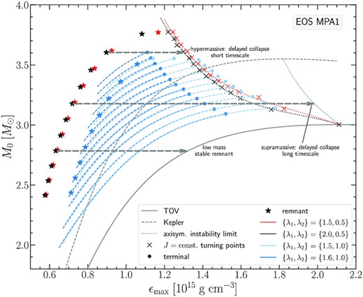
Rest mass M0 versus maximum energy density ϵmax for the MPA1 EOS. The different sequences are as in Fig. 10. The grey dashed arrows indicate possible evolutionary paths of merger remnants as they lose angular momentum, if mass-loss is neglected.
Physical quantities for equilibrium remnant models constructed with the MPA1 EOS and different choices of rotation law parameters. The different quantities are defined as in Table 5.
| rp/re | ϵc(× 1015) | ϵmax(× 1015) | M | M0 | J | T/|W| | Ωc | Ωmax | Ωe | ΩK | Re | re | GRV3 |
|---|---|---|---|---|---|---|---|---|---|---|---|---|---|
| {λ1, λ2} | |$(\mathrm{g \, cm^{-3}})$| | |$(\mathrm{g \, cm^{-3}})$| | |$(\, \mathrm{M}_\odot )$| | |$(\, \mathrm{M}_\odot )$| | |$(\frac{G M_{\odot }^2}{c})$| | (rad ms−1) | (rad ms−1) | (rad ms−1) | (rad ms−1) | (km) | (km) | (× 10−5) | |
| {2.0, 0.5} | |||||||||||||
| 0.3065 | 0.4260 | 0.5761 | 2.2 | 2.4131 | 4.4180 | 0.2205 | 8.4137 | 16.8274 | 4.2068 | 7.9797 | 17.1615 | 13.3944 | 14.4367 |
| 0.2985 | 0.4285 | 0.5925 | 2.3 | 2.5346 | 4.7867 | 0.2222 | 8.6843 | 17.3686 | 4.3421 | 8.1391 | 17.1622 | 13.2038 | 13.8202 |
| 0.2934 | 0.4350 | 0.6110 | 2.4 | 2.6578 | 5.1565 | 0.2232 | 8.9821 | 17.9643 | 4.4911 | 8.3202 | 17.1186 | 12.9678 | 13.4671 |
| 0.2911 | 0.4465 | 0.6324 | 2.5 | 2.7835 | 5.5263 | 0.2236 | 9.3157 | 18.6314 | 4.6578 | 8.5283 | 17.0270 | 12.6816 | 13.8714 |
| 0.2915 | 0.4641 | 0.6573 | 2.6 | 2.9123 | 5.8965 | 0.2234 | 9.6920 | 19.3842 | 4.8460 | 8.7668 | 16.8878 | 12.3448 | 9.5482 |
| 0.2936 | 0.4861 | 0.6855 | 2.7 | 3.0430 | 6.2685 | 0.2230 | 10.1113 | 20.2226 | 5.0556 | 9.0301 | 16.7122 | 11.9693 | 8.2679 |
| 0.2975 | 0.5140 | 0.7187 | 2.8 | 3.1769 | 6.6425 | 0.2221 | 10.5906 | 21.1815 | 5.2953 | 9.3294 | 16.4912 | 11.5439 | 7.1198 |
| 0.3042 | 0.5510 | 0.7608 | 2.9 | 3.3153 | 7.0144 | 0.2207 | 11.1621 | 22.3244 | 5.5811 | 9.6864 | 16.2037 | 11.0456 | 8.3531 |
| 0.3121 | 0.5970 | 0.8154 | 3.0 | 3.4568 | 7.3878 | 0.2190 | 11.8549 | 23.7102 | 5.9274 | 10.1095 | 15.8508 | 10.4744 | 8.6592 |
| 0.3224 | 0.6610 | 0.8970 | 3.1 | 3.6037 | 7.7617 | 0.2169 | 12.7936 | 25.5878 | 6.3968 | 10.6687 | 15.3706 | 9.7608 | 7.3993 |
| 0.3367 | 0.7900 | 1.0824 | 3.2 | 3.7578 | 8.1352 | 0.2144 | 14.6102 | 29.2249 | 7.3051 | 11.6946 | 14.4834 | 8.5922 | 8.1130 |
| {1.5, 0.5} | |||||||||||||
| 0.3866 | 0.5380 | 0.5819 | 2.2 | 2.4205 | 4.4179 | 0.2178 | 8.9666 | 13.4499 | 4.4833 | 8.0489 | 17.0026 | 13.2377 | 15.8326 |
| 0.3816 | 0.5485 | 0.5991 | 2.3 | 2.5424 | 4.7867 | 0.2196 | 9.2482 | 13.8723 | 4.6241 | 8.2177 | 16.9911 | 13.0347 | 12.0241 |
| 0.3788 | 0.5625 | 0.6187 | 2.4 | 2.6666 | 5.1565 | 0.2207 | 9.5562 | 14.3342 | 4.7781 | 8.4102 | 16.9350 | 12.7851 | 12.1648 |
| 0.3784 | 0.5805 | 0.6414 | 2.5 | 2.7934 | 5.5264 | 0.2210 | 9.8964 | 14.8445 | 4.9482 | 8.6295 | 16.8339 | 12.4881 | 12.2902 |
| 0.3795 | 0.6020 | 0.6671 | 2.6 | 2.9221 | 5.8966 | 0.2208 | 10.2697 | 15.4046 | 5.1349 | 8.8718 | 16.6965 | 12.1527 | 10.9684 |
| 0.3824 | 0.6280 | 0.6969 | 2.7 | 3.0541 | 6.2685 | 0.2200 | 10.6889 | 16.0334 | 5.3445 | 9.1453 | 16.5173 | 11.7716 | 8.2365 |
| 0.3866 | 0.6590 | 0.7321 | 2.8 | 3.1888 | 6.6425 | 0.2189 | 11.1632 | 16.7448 | 5.5816 | 9.4523 | 16.2976 | 11.3458 | 7.3561 |
| 0.3927 | 0.6980 | 0.7763 | 2.9 | 3.3274 | 7.0144 | 0.2173 | 11.7225 | 17.5838 | 5.8613 | 9.8135 | 16.0180 | 10.8541 | 7.8691 |
| 0.4004 | 0.7485 | 0.8350 | 3.0 | 3.4700 | 7.3878 | 0.2153 | 12.4110 | 18.6165 | 6.2055 | 10.2491 | 15.6659 | 10.2810 | 9.1894 |
| 0.4099 | 0.8240 | 0.9246 | 3.1 | 3.6177 | 7.7617 | 0.2129 | 13.3604 | 20.0406 | 6.6802 | 10.8311 | 15.1810 | 9.5587 | 7.8279 |
| 0.4228 | 1.0200 | 1.1673 | 3.2 | 3.7707 | 8.1352 | 0.2105 | 15.5006 | 23.2512 | 7.7503 | 12.0506 | 14.1554 | 8.2317 | 9.7803 |
| {1.6, 1.0} | |||||||||||||
| 0.4842 | 0.7127 | 0.7127 | 2.2 | 2.4349 | 4.4180 | 0.2026 | 5.5146 | 8.8233 | 5.5146 | 7.1943 | 18.1611 | 14.4404 | 14.5244 |
| 0.4872 | 0.7343 | 0.7343 | 2.3 | 2.5591 | 4.7867 | 0.2041 | 5.6713 | 9.0741 | 5.6713 | 7.4547 | 17.9811 | 14.0644 | 13.5309 |
| 0.4917 | 0.7588 | 0.7588 | 2.4 | 2.6855 | 5.1565 | 0.2048 | 5.8389 | 9.3422 | 5.8389 | 7.7359 | 17.7683 | 13.6528 | 12.4246 |
| 0.4974 | 0.7872 | 0.7872 | 2.5 | 2.8143 | 5.5264 | 0.2047 | 6.0192 | 9.6308 | 6.0192 | 8.0385 | 17.5258 | 13.2088 | 11.9574 |
| 0.5045 | 0.8206 | 0.8206 | 2.6 | 2.9460 | 5.8966 | 0.2040 | 6.2158 | 9.9452 | 6.2158 | 8.3660 | 17.2534 | 12.7314 | 11.2757 |
| 0.5125 | 0.8604 | 0.8604 | 2.7 | 3.0807 | 6.2686 | 0.2028 | 6.4319 | 10.2911 | 6.4319 | 8.7184 | 16.9557 | 12.2248 | 11.8631 |
| 0.5215 | 0.9088 | 0.9088 | 2.8 | 3.2183 | 6.6425 | 0.2012 | 6.6744 | 10.6790 | 6.6744 | 9.1027 | 16.6285 | 11.6841 | 11.0840 |
| 0.5322 | 0.9712 | 0.9712 | 2.9 | 3.3599 | 7.0144 | 0.1991 | 6.9594 | 11.1351 | 6.9594 | 9.5434 | 16.2476 | 11.0829 | 12.1694 |
| 0.5443 | 1.0582 | 1.0582 | 3.0 | 3.5061 | 7.3878 | 0.1967 | 7.3166 | 11.7066 | 7.3166 | 10.0705 | 15.7915 | 10.3956 | 13.0393 |
We note that no remnant models are located for these lower J-constant sequences, since their lower masses (implying a binary total mass |$M_\text{tot} \lt 2.2 \, \mathrm{M}_\odot$|) would make them irrelevant for this study. The arrows in Fig. 29 approximate the evolutionary path of remnants as they lose angular momentum (assuming constant rest mass). A remnant will evolve towards larger densities and higher compactness, as its angular momentum decreases. In addition, the rotation law may also evolve in time. Three representative evolutionary paths are shown, resulting in a delayed collapse to a black hole on a short time-scale (when the remnant is hypermassive); a delayed collapse on a longer time-scale (when the remnant is supramassive and can still exist as a uniformly rotating model); and a stable remnant (when its mass is smaller than the maximum mass for non-rotating models).
The description of post-merger remnants as quasi-equilibrium models has applications in the interpretation of the post-merger GW spectrum; in the study of the threshold mass to prompt collapse; in the construction of universal or empirical relations between properties of the remnants and properties of non-rotating models; and in modelling of processes taking place on longer time-scales that are relevant for multimessenger follow-up studies of GW detections (Ciolfi et al. 2021; Rosati et al. 2021). We plan to elaborate further on these aspects in future work.
ACKNOWLEDGEMENTS
We thank Andreas Bauswein, John Friedman, Dimitrios Papadopoulos, and Christos Tsagas for helpful discussions and comments. We also thank the anonymous referee for providing useful comments that improved the final manuscript. PI gratefully acknowledges support by a Virgo-EGO Scientific Forum (VESF) PhD fellowship. NS acknowledges support by the COST actions CA16214 ‘PHAROS’, CA16104 ‘GWVerse’, and CA18108 ‘QG-MM’. The authors gratefully acknowledge the Italian Instituto Nazionale di Fisica Nucleare (INFN), the French Centre National de la Recherche Scientifique (CNRS), and the Netherlands Organization for Scientific Research, for the construction and operation of the Virgo detector and the creation and support of the EGO consortium.
DATA AVAILABILITY
The data underlying this article are available in the article.
Footnotes
We note that in the simulations of Bauswein et al. (2020) the EOS table used for DD2 provided temperature dependence, whereas the APR and MPA1 were used in a hybrid form (zero-temperature EOS supplemented by an approximate thermal part).
We note that the numerical method used in the rns code does not discriminate between different types of models with same axial ratio, central or maximum density and differential rotation law, so that the numerical iterations can alternate between two different solutions, instead of converging to a specific one.
Note that we do not discuss Type B and Type D solutions of Ansorg et al. (2009) in this study. Depending on the choice of parameters, Type B solutions can co-exist with those of Type A and Type D with those of Type C.
This holds as a rule of thumb, barring a possible numerical stiffness encountered for high J values and weak differential rotation (see discussion in Section 3.2).
The remnant sequences are interpolated using the package PchipInterpolator from the SciPy library (Virtanen et al. 2020). This package incorporates the Piecewise Cubic Hermite Interpolating Polynomial (PCHIP) algorithm (Fritsch & Butland 1984) and additionally provides an extrapolation option. The latter uses the monotonic cubic spline from the last interval of the data to find the value of the points in the extrapolated range.
The TOV core equivalent, is defined as the ‘bulk’ of a TOV star, meaning the region enclosed by the isodensity surface with the maximum compactness CV = Mb/RV, where V is the total enclosed proper 3-volume by the isodensity surface, Mb is the respective total baryon mass and RV is a volumetric radius defined through |$V = \frac{4}{3} \pi R_V^3$|. See Kastaun et al. (2016) for further details.
REFERENCES
APPENDIX: COMPARISON OF ANGULAR MOMENTUM EMPIRICAL RELATIONS
In this appendix, we present a more detailed comparison for the empirical relations (7) and (8) discussed in Section 2.5 that were used to estimate the angular momentum at the time of merger.
In Fig. A1 the two angular momentum empirical relations (7) and (A1) are shown for the DD2 EOS. An Mtot ranging from |$2.2 \, \mathrm{M}_\odot$| to |$3.3 \, \mathrm{M}_\odot$| is assumed. Note that the threshold mass for prompt collapse to a black hole for this particular EOS is |$M_\text{thres} \simeq 3.325 \, \mathrm{M}_\odot$| as reported from numerical simulations by Bauswein et al. (2020, Supplementary Material). In equation (A1) we have set RNS = 13.1 km, which is a typical circumferential radius value for progenitor neutron stars constructed with the DD2 EOS (see Fig. 1). The two curves show very good agreement, deviating for the most part at the 2.5 per cent level and at the 5 per cent level only for very low mass remnants.
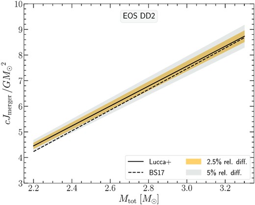
Comparison of empirical relations for the angular momentum at the time of merger, Jmerger versus the total binary mass, Mtot, for the DD2 EOS. The solid line represents the empirical relation from Lucca et al. (2021) cast into the form used in Bauswein & Stergioulas, i.e. equation (A1), while the dashed line represents the empirical relation from Bauswein & Stergioulas (2017), i.e. equation (7). The orange and grey filled areas denote the relative difference bands at the 2.5 per cent and 5 per cent level, respectively.
To investigate further the two angular momentum empirical formulas, we consider six zero-temperature, tabulated EOS, namely APR, DD2, and MPA1 already mentioned in Section 2.4 with the addition of SFHx (Steiner, Hempel & Fischer 2013), SLy4 (Douchin & Haensel 2001), and WFF1 EOS (Wiringa, Fiks & Fabrocini 1988). For each EOS, we consider a remnant mass range starting from |$2.2 \, \mathrm{M}_\odot$| and increasing with a step of |$0.1 \, \mathrm{M}_\odot$| up to approximately the threshold mass value Mthres, as the latter is reported in Bauswein et al. (2020). Constructing the corresponding non-rotating progenitor models with MNS = Mtot/2, we then use the empirical relations (7) and (8) to get predictions for the value of Jmerger from each formula.
Tables A1, A2, A3, A4, A5, and A6 report the Jmerger estimates from the Bauswein & Stergioulas (2017) and Lucca et al. (2021) expressions. For the EOS DD2, MPA1, SFHx, and SLy4 excellent agreement is noticed, as the relative difference ranges from |$\sim 0.5{{\ \rm per\ cent}}$| up to |$\sim 5{{\ \rm per\ cent}}$|. For the APR EOS, somewhat larger deviations (|$\gt 6{{\ \rm per\ cent}}$|) are noticed for remnants with masses over |$2.6 \, \mathrm{M}_\odot$|, with the Bauswein & Stergioulas (2017) approximate formula predicting larger angular momentum values. The picture is similar for the WFF1 EOS, with the deviations augmented to the 10 per cent level.
Angular momentum predictions from two different empirical relations, for the APR EOS. The total binary mass Mtot, the progenitor masses MNS = Mtot/2, the equatorial circumferential radii RNS, and the values of compactness CNS are shown. The Jmerger columns correspond to angular momentum predictions from the empirical relations reported in Bauswein & Stergioulas (2017) (abbreviated as BS17) and Lucca et al. (2021) (abbreviated as Lucca+). The last column reports the absolute values of the relative difference between the Jmerger predictions. Note that Mtot is terminated approximately at the Mthres value, as the latter is reported in Bauswein et al. (2020).
| Mtot | MNS | RNS | CNS | |$\frac{cJ_\text{merger}}{G M_\odot ^2}$| | |$\frac{cJ_\text{merger}}{G M_\odot ^2}$| | rel. diff. |
|---|---|---|---|---|---|---|
| (M⊙) | (M⊙) | (km) | (BS17) | (Lucca+) | (per cent) | |
| 2.20 | 1.10 | 11.3774 | 0.143 | 4.4165 | 4.3365 | 1.85 |
| 2.30 | 1.15 | 11.3735 | 0.149 | 4.8203 | 4.6733 | 3.14 |
| 2.40 | 1.20 | 11.3689 | 0.156 | 5.2248 | 5.0105 | 4.28 |
| 2.50 | 1.25 | 11.3634 | 0.162 | 5.6290 | 5.3469 | 5.28 |
| 2.60 | 1.30 | 11.3567 | 0.169 | 6.0324 | 5.6821 | 6.17 |
| 2.70 | 1.35 | 11.3482 | 0.176 | 6.4372 | 6.0175 | 6.97 |
| 2.80 | 1.40 | 11.3379 | 0.182 | 6.8417 | 6.3517 | 7.71 |
| 2.84 | 1.42 | 11.3331 | 0.185 | 7.0021 | 6.4838 | 7.99 |
Same as Table A1 for the DD2 EOS.
| Mtot | MNS | RNS | CNS | |$\frac{cJ_\text{merger}}{G M_\odot ^2}$| | |$\frac{cJ_\text{merger}}{G M_\odot ^2}$| | rel. diff. |
|---|---|---|---|---|---|---|
| (M⊙) | (M⊙) | (km) | (BS17) | (Lucca+) | (per cent) | |
| 2.20 | 1.10 | 13.0385 | 0.125 | 4.2314 | 4.4513 | 4.94 |
| 2.30 | 1.15 | 13.0594 | 0.130 | 4.6361 | 4.8401 | 4.21 |
| 2.40 | 1.20 | 13.0795 | 0.135 | 5.0379 | 5.2273 | 3.62 |
| 2.50 | 1.25 | 13.0985 | 0.141 | 5.4448 | 5.6203 | 3.12 |
| 2.60 | 1.30 | 13.1161 | 0.146 | 5.8481 | 6.0109 | 2.71 |
| 2.70 | 1.35 | 13.1320 | 0.152 | 6.2519 | 6.4027 | 2.36 |
| 2.80 | 1.40 | 13.1460 | 0.157 | 6.6561 | 6.7954 | 2.05 |
| 2.90 | 1.45 | 13.1578 | 0.163 | 7.0607 | 7.1888 | 1.78 |
| 3.00 | 1.50 | 13.1672 | 0.168 | 7.4648 | 7.5818 | 1.54 |
| 3.10 | 1.55 | 13.1743 | 0.174 | 7.8683 | 7.9740 | 1.33 |
| 3.20 | 1.60 | 13.1784 | 0.179 | 8.2734 | 8.3673 | 1.12 |
| 3.28 | 1.64 | 13.1795 | 0.184 | 8.5960 | 8.6800 | 0.97 |
Same as Table A1 for the MPA1 EOS.
| Mtot | MNS | RNS | CNS | |$\frac{cJ_\text{merger}}{G M_\odot ^2}$| | |$\frac{cJ_\text{merger}}{G M_\odot ^2}$| | rel. diff. |
|---|---|---|---|---|---|---|
| (M⊙) | (M⊙) | (km) | (BS17) | (Lucca+) | (per cent) | |
| 2.2 | 1.10 | 12.3276 | 0.132 | 4.3011 | 4.4180 | 2.65 |
| 2.3 | 1.15 | 12.3498 | 0.137 | 4.7060 | 4.7867 | 1.68 |
| 2.4 | 1.20 | 12.3711 | 0.143 | 5.1109 | 5.1565 | 0.88 |
| 2.5 | 1.25 | 12.3913 | 0.149 | 5.5146 | 5.5264 | 0.21 |
| 2.6 | 1.30 | 12.4102 | 0.155 | 5.9177 | 5.8966 | 0.36 |
| 2.7 | 1.35 | 12.4277 | 0.160 | 6.3217 | 6.2685 | 0.85 |
| 2.8 | 1.40 | 12.4437 | 0.166 | 6.7273 | 6.6425 | 1.28 |
| 2.9 | 1.45 | 12.4579 | 0.172 | 7.1300 | 7.0144 | 1.65 |
| 3.0 | 1.50 | 12.4702 | 0.178 | 7.5342 | 7.3878 | 1.98 |
| 3.1 | 1.55 | 12.4805 | 0.183 | 7.9387 | 7.7616 | 2.28 |
| 3.2 | 1.60 | 12.4885 | 0.189 | 8.3431 | 8.1352 | 2.56 |
Same as Table A1 for the SFHx EOS.
| Mtot | MNS | RNS | CNS | |$\frac{cJ_\text{merger}}{G M_\odot ^2}$| | |$\frac{cJ_\text{merger}}{G M_\odot ^2}$| | rel. diff. |
|---|---|---|---|---|---|---|
| (M⊙) | (M⊙) | (km) | (BS17) | (Lucca+) | (per cent) | |
| 2.2 | 1.10 | 11.8206 | 0.137 | 4.3573 | 4.3801 | 0.52 |
| 2.3 | 1.15 | 11.8451 | 0.143 | 4.7619 | 4.7342 | 0.58 |
| 2.4 | 1.20 | 11.8649 | 0.149 | 5.1649 | 5.0877 | 1.52 |
| 2.5 | 1.25 | 11.8832 | 0.155 | 5.5700 | 5.4439 | 2.32 |
| 2.6 | 1.30 | 11.8965 | 0.161 | 5.9736 | 5.7989 | 3.01 |
| 2.7 | 1.35 | 11.9073 | 0.167 | 6.3775 | 6.1543 | 3.63 |
| 2.8 | 1.40 | 11.9140 | 0.173 | 6.7813 | 6.5092 | 4.18 |
| 2.9 | 1.45 | 11.9174 | 0.180 | 7.1856 | 6.8640 | 4.69 |
| 3.0 | 1.50 | 11.9151 | 0.186 | 7.5901 | 7.2173 | 5.17 |
Same as Table A1 for the SLy4 EOS.
| Mtot | MNS | RNS | CNS | |$\frac{cJ_\text{merger}}{G M_\odot ^2}$| | |$\frac{cJ_\text{merger}}{G M_\odot ^2}$| | rel. diff. |
|---|---|---|---|---|---|---|
| (M⊙) | (M⊙) | (km) | (BS17) | (Lucca+) | (per cent) | |
| 2.2 | 1.10 | 11.8588 | 0.137 | 4.3833 | 4.3831 | 0.01 |
| 2.3 | 1.15 | 11.8421 | 0.143 | 4.7886 | 4.7341 | 1.15 |
| 2.4 | 1.20 | 11.8238 | 0.150 | 5.1916 | 5.0820 | 2.16 |
| 2.5 | 1.25 | 11.8033 | 0.156 | 5.5957 | 5.4292 | 3.07 |
| 2.6 | 1.30 | 11.7800 | 0.163 | 6.0007 | 5.7756 | 3.90 |
| 2.7 | 1.35 | 11.7537 | 0.170 | 6.4039 | 6.1181 | 4.67 |
| 2.8 | 1.40 | 11.7239 | 0.176 | 6.8078 | 6.4588 | 5.40 |
Same as Table A1 for the WFF1 EOS.
| Mtot | MNS | RNS | CNS | |$\frac{cJ_\text{merger}}{G M_\odot ^2}$| | |$\frac{cJ_\text{merger}}{G M_\odot ^2}$| | rel. diff. |
|---|---|---|---|---|---|---|
| (M⊙) | (M⊙) | (km) | (BS17) | (Lucca+) | (per cent) | |
| 2.2 | 1.10 | 10.3754 | 0.157 | 4.5093 | 4.2029 | 7.29 |
| 2.3 | 1.15 | 10.3840 | 0.164 | 4.9126 | 4.5119 | 8.88 |
| 2.4 | 1.20 | 10.3911 | 0.171 | 5.3178 | 4.8225 | 10.27 |
| 2.5 | 1.25 | 10.3970 | 0.178 | 5.7222 | 5.1326 | 11.49 |
| 2.6 | 1.30 | 10.4010 | 0.185 | 6.1260 | 5.4420 | 12.57 |
| 2.7 | 1.35 | 10.4034 | 0.192 | 6.5297 | 5.7512 | 13.54 |
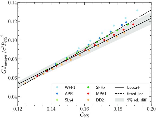
Angular momentum at the time of merger, Jmerger, normalized by the TOV progenitor neutron star circumferential radius squared, |$R_\text{NS}^2$| versus the corresponding compactness CNS (equal mass binaries are assumed). The filled circles correspond to the data presented in Tables A1–A6, i.e. they represent Jmerger predictions (normalized by |$R_\text{NS}^2$|) following the empirical formula in Bauswein & Stergioulas (2017) for remnants with different EOS and their correlation with the respective TOV progenitors’ compactness CNS. The dashed line is a linear fit to the filled circles data, i.e equation (A2), the solid line represents the empirical formula of Lucca et al. (2021), i.e. equation (8), and the grey filled area the 5 per cent relative difference band.
Overall, the agreement between the empirical formulas from Bauswein & Stergioulas (2017) and Lucca et al. (2021) at a level of a few per cent is notable, given that (i) they are independent analyses of different numerical simulations data sets and (ii) the formula appearing in Bauswein & Stergioulas was a benchmark for the DD2 EOS with an added approximate treatment to describe other EOS. In fact, since one cannot be certain that the specifics of the angular momentum extraction were performed in an identical way between the two works, the actual agreement could prove to be even better. In any case, an accuracy of a few per cent is adequate to get useful insights into merger remnants properties with equilibrium models.
