


ABSTRACT
Direction-dependent calibration of widefield radio interferometers estimates the systematic errors, along with multiple directions in the sky. This is necessary because with most systematic errors, which are caused by effects such as the ionosphere or the receiver beam shape, there is a significant spatial variation. Fortunately, there is some deterministic behaviour of these variations in most situations. We enforce this underlying smooth spatial behaviour of systematic errors as an additional constraint on to spectrally constrained direction-dependent calibration. Using both analysis and simulations, we show that this additional spatial constraint improves the performance of multifrequency direction-dependent calibration.
1 INTRODUCTION
One limitation for improving the quality of data obtained by modern widefield radio interferometric arrays is the systematic errors affecting the data. Calibration, or the determination and removal of systematic errors, is therefore a crucial data processing step in radio interferometry. When the observing field of view is wide, especially in low-frequency radio astronomy, the systematic errors vary with the direction in the sky and therefore, direction-dependent calibration is necessary. Numerous techniques exist for direction-dependent calibration and Cotton & Mauch (2021) give a comprehensive overview of the current state of the art.
By definition, ‘direction dependence’ implies that the systematic errors are spatially variable (in addition to temporal and spectral variability). We can categorize the spatial variation into two groups. In deterministic variability, the spatial variations are smooth and contiguous and they can be described by a simple model. Examples for such variations are the systematic errors caused by the main lobe of a phased array beam or the refraction caused by a benign ionosphere. The second category of spatial variability is random or stochastic. In this case, a simple model will not be able to completely describe the systematic errors. The side lobe patterns of a phased array beam or scintillation caused by a turbulent ionosphere are two examples for the causes of stochastic direction-dependent errors. In practice, the systematic errors are a combination of both deterministic and stochastic components, and the amount of each component is unknown.
Multifrequency direction-dependent calibration has already been improved by using the spectral smoothness of systematic errors as a regularizer (Yatawatta 2015; Brossard et al. 2018; Ollier et al. 2018; Yatawatta et al. 2018, 2020). Improving on this, in this paper, we add an implicit model for the spatial dependence of systematic errors as an extra regularizer. We favour an implicit model over an explicit model because the amount of deterministic behaviour of the direction dependence is unknown to us. For one observation, we might get well-defined direction dependence of systematic errors while for another observation, we might get completely random and uncorrelated direction dependence. Our spatial model will adapt itself to each observation according to this dichotomy. We use the calibration solutions for each direction to bootstrap our spatial model. In order to prevent overfitting, we pass the solutions through an information bottleneck by using elastic net regression (Zou & Hastie 2005) to construct the spatial model.
Explicit models have already being used to improve direction-dependent calibration, for example by modelling ionospheric effects (Cotton 2007; Mitchell et al. 2008; Intema et al. 2009; Arora et al. 2016; Albert et al. 2020) or beam effects (Bhatnagar et al. 2008; Yatawatta 2018b; Cotton & Mauch 2021). Most of these methods are not scalable to process multifrequency data in a distributed computer. Instead of having a model with both spectral and spatial dependence, we use disjoint models and separate constraints for spectral dependence and spatial dependence. We use consensus optimization (Boyd et al. 2011) and extend our previous work (Yatawatta 2020) to incorporate the spatial constraint as an extension to a model derived by federated averaging (McMahan et al. 2016). In this manner, we are able to incorporate both spectral and spatial constraints without losing scalability in processing multifrequency data in a distributed computer. However, since we use an implicit model, relating this model to actual physical phenomena, such as the ionosphere and the beam shape, is more involved and is a drawback of our approach.
The remainder of the paper is organized as follows. In Section 2, we define the radio interferometric data model and describe our spatially constrained distributed calibration algorithm. In Section 3, we derive performance criteria based on the influence function (Hampel et al. 1986; Yatawatta 2019a). We perform simulations and present the results in Section 4 to illustrate the improvement due to the spatial constraint. Finally, we draw our conclusions in Section 5.
Notation: Lower case bold letters refer to column vectors (e.g. y). Upper case bold letters refer to matrices (e.g. C). Unless otherwise stated, all parameters are complex numbers. The set of complex numbers is given as |${\mathbb {C}}$| and the set of real numbers as |${\mathbb {R}}$|. The matrix inverse, pseudo-inverse, transpose, Hermitian transpose, and conjugation are referred to as (·)−1, (·)†, (·)T, (·)H, (·)⋆, respectively. The matrix Kronecker product is given by ⊗. The vectorized representation of a matrix is given by vec(·). The identity matrix of size N is given by IN. All logarithms are to the base e, unless stated otherwise. The Frobenius norm is given by ‖ · ‖.
2 SPECTRALLY AND SPATIALLY CONSTRAINED CALIBRATION
We use the alternating direction method of multipliers (ADMM) algorithm (Boyd et al. 2011) to solve (8) and the pseudo-code is given in Algorithm 1. As in (Yatawatta 2015), we consider a fusion centre that is connected to a set of worker nodes to implement Algorithm 1. Most of the computations are done in parallel at all the worker nodes.
Spatially constrained distributed calibration
 |
|
Spatially constrained distributed calibration
|
|
3 PERFORMANCE ANALYSIS
4 SIMULATIONS
We simulate an interferometric array with N = 62 stations, using phased array beams, such as LOFAR. The duration of the observation is 10 min, divided into samples with 10 s integration, so in total 60 time samples. We use P = 8 frequencies, equally spaced in the range [115, 185] MHz. The calibration is performed using every Δt = 10 time samples, or 100 s of data.
The sky model consists of K = 10 point-sources in the sky that are being calibrated, with their positions randomly chosen within a 30 deg radius from the field centre. Their intrinsic fluxes are randomly chosen in the range [100, 1000] Jy and their spectral indices are randomly chosen from a standard normal distribution. An additional 400 weak sources (both point sources and Gaussians) are randomly positioned across a 16 × 16 square degrees field of view. Their intensities are uniform-randomly selected from [0.01,0.5] Jy with flat spectra. All the aforementioned sources are unpolarized. A model for diffuse structure (with Stokes I, Q, and U fluxes) based on shapelets are also added to the simulation. The simulation incorporates beam effects, both the dipole beam and the station beam.
The systematic errors, i.e. |${\bf J}_{pkf_i}$| in (1), are simulated for the K = 10 sources as follows. For any given p, we simulate the eight values of |${\bf J}_{pkf_i}$| for the central frequency and for k = 1. We multiply this with a random third-order polynomial in frequency to get the frequency variation. We also multiply this value with a random sinusoidal in time to get time variability. We get spatial variability by propagating |${\bf J}_{pkf_i}$| for k = 1 to other directions (or other values of k). We do this by generating random planes in l, m coordinates (such as a1l + a2m + a3 where a1, a2, a3 are generated from a standard normal distribution) and multiplying the eight values of |${\bf J}_{pkf_i}$| for k = 1 with these random planes evaluated at the l, m coordinates of each direction. Finally, an additional random value drawn from a standard normal distribution is added to the values of |${\bf J}_{pkf_i}$| at each k.
The noise Npq in (1) is generated as complex zero mean Gaussian distributed elements and is added to the simulated signal with a signal to noise ratio of 0.05. An example of a simulation is shown in Fig. 1(a).
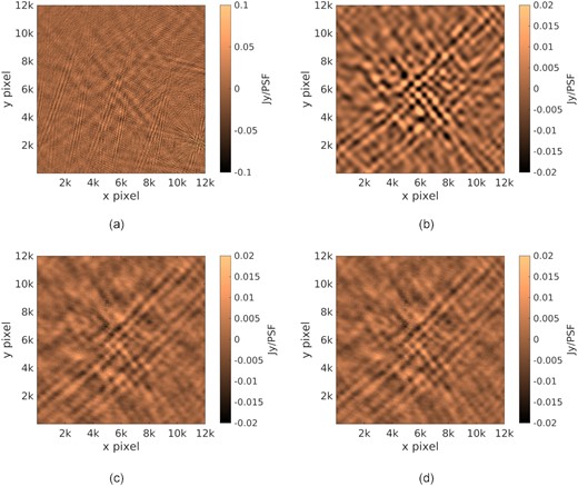
Sample images (not deconvolved) made using simulated data, covering about 13.3 × 13.3 square degrees in the sky. (a) The image before calibration. (b) The diffuse sky and the weak sources that are hidden in the simulated data. (c) The residual image after calibration, without using spatial regularization. (d) The residual image after calibration, with spatial regularization. Both (c) and (d) reveal the weak sky shown in (b), but the intensity is much less.
We perform calibration using a third order Bernstein polynomial in frequency for consensus. The spectral regularization parameter ρ is chosen with a peak value of 300 and scaled according to the apparent flux of each of the K = 10 directions being calibrated. When spatial regularization is enabled, we use a spherical harmonic basis with order 3 (giving G = 9 basis functions). The spatial regularization parameter α is set equal to ρ for each direction. We use 20 ADMM iterations and the spatial model is updated at every tenth iteration (if enabled). The elastic net regression to update the spatial model uses λ = 0.01 and μ = 10−4 as the L2 and L1 constraints and we use 40 FISTA iterations.
We measure the performance of calibration by measuring the suppression of the unmodelled weak sources in the sky due to calibration. As seen in Fig. 1(b), we can simulate only the weak sky, and compare this to the residual images made after calibration. Numerically, we can cross-correlate for example Fig. 1(b) with Fig. 1(c) or Fig. 1(d). We show the correlation coefficient calculated this way for several simulations in Fig. 2. Note that, calibration, along K = 10 directions with only 100 s of data, is not well constrained. None the less, we see from Fig. 2 that introducing spatial constraints into the problem increases the correlation of the residual with the weak sky. In other words, the spatial constraints decreases the loss of unmodelled structure in the sky.
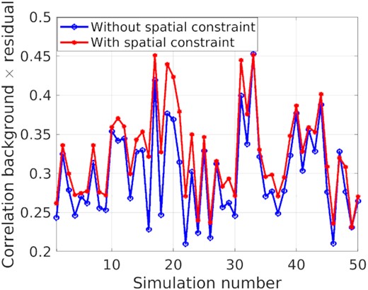
The correlation of the residual maps with the weak sky signal (in Stokes I, Q, and U). With spatial constraint, we can increase the correlation from about 30 per cent to 34 per cent on average.
We use the influence function derived in Section 3 to explain the behaviour in Fig. 2. We show the plots of 1 + λi with i in Fig. 3 for calibration with no regularization (ρ = α = 0), with only spectral regularization (ρ > 0, α = 0), and with both spectral and spatial regularization (ρ > 0, α > 0). We see that calibration with both spatial and spectral regularization gives the curve of 1 + λi with the lowest area above the curve (or the epigraph). In other words, the number of degrees of freedom consumed by calibration with both spectral and spatial regularization is the lowest. This also means that the loss of weak signals due to calibration is the lowest for both spectral and spatial regularized calibration, as we show in Fig. 2. However, the improvement depends on the actual amount of deterministic variability of systematic errors with direction and the appropriate selection of regularization parameters ρ, α.
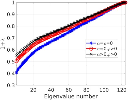
Eigenvalue plots for the influence function of calibration with (i) no regularization (ii) spectral regularization, and (iii) both spectral and spatial regularization. The epigraph of the curve is lowest with both spectral and spatial regularization.
5 CONCLUSIONS
We have presented a method to incorporate spatial constraints to spectrally constrained direction-dependent calibration. Whenever the direction-dependent errors have a deterministic spatial variation, we can bootstrap a spatial model. With only a small increase in computations, we are able to improve the performance of spectrally constrained calibration. The improvement depends on the actual spatial variation of systematic errors, i.e. whether it is deterministic or stochastic. Moreover, the appropriate selection of the regularization factor α is also affecting the final result. Future work will focus on automating the determination of optimal regularization and modelling parameters, for example, by using reinforcement learning.
ACKNOWLEDGEMENTS
We thank Chris Jordan for the careful review and valuable comments.
DATA AVAILABILITY
Ready-to-use software based on this work and test data are available online.1
