Revised event rates for extreme and extremely large mass-ratio inspirals

Vázquez-Aceves, Verónica; Zwick, Lorenz; Bortolas, Elisa; Capelo, Pedro R; Amaro Seoane, Pau; Mayer, Lucio; Chen, Xian

doi:10.1093/mnras/stab3485

ABSTRACT

One of the main targets of the Laser Interferometer Space Antenna (LISA) is the detection of extreme mass-ratio inspirals (EMRIs) and extremely large mass-ratio inspirals (X-MRIs). Their orbits are expected to be highly eccentric and relativistic when entering the LISA band. Under these circumstances, the inspiral time-scale given by Peters’ formula loses precision and the shift of the last-stable orbit (LSO) caused by the massive black hole spin could influence the event rates estimate. We re-derive EMRIs and X-MRIs event rates by implementing two different versions of a Kerr loss-cone angle that includes the shift in the LSO, and a corrected version of Peters’ time-scale that accounts for eccentricity evolution, 1.5 post-Newtonian hereditary fluxes, and spin-orbit coupling. The main findings of our study are summarized as follows: (1) implementing a Kerr loss-cone changes the event rates by a factor ranging between 0.9 and 1.1; (2) the high-eccentricity limit of Peters’ formula offers a reliable inspiral time-scale for EMRIs and X-MRIs, resulting in an event-rate estimate that deviates by a factor of about 0.9–3 when compared to event rates computed with the corrected version of Peters’ time-scale and the usual loss-cone definition. (3) Event-rate estimates for systems with a wide range of eccentricities should be revised. Peters’ formula overestimates the inspiral rates of highly eccentric systems by a factor of about 8–30 compared to the corrected values. Besides, for e₀ ≲ 0.8, implementing the corrected version of Peters’ formula is necessary to obtain accurate estimates.

black hole physics, gravitational waves, methods: analytical

1 INTRODUCTION

Massive black holes (MBHs) at the centre of galaxies can capture compact objects – such as stellar-mass BHs, white dwarfs (WDs), neutron stars (NSs), and even brown dwarfs (BDs) – that can either suffer a direct plunge or slowly inspiral to the event horizon without being disrupted. The latter events are known as extreme mass-ratio inspirals (EMRIs) when the mass ratio q between the compact object and the MBH is of the order of 10⁻⁴, and as extremely large mass-ratio inspirals (X-MRIs) when q ∼ 10⁻⁸. During the inspiral process, the binary would emit low-frequency gravitational waves (GWs) that space-borne detectors like the Laser Interferometer Space Antenna (LISA) can detect (Barack & Cutler 2004; Amaro-Seoane et al. 2012; Klein et al. 2016; Babak et al. 2017; Amaro-Seoane 2018; Barack et al. 2019), providing detailed information about the binary and the surrounding space–time that is impossible to obtain via electromagnetic observations. Such detections would allow testing general relativity with exceptional accuracy; therefore, it is crucial to accurately estimate the event rates and the characteristics of inspiral processes.

The eccentricity of an EMRI or X-MRI when entering the LISA band depends on the formation channel. There are two basic formation scenarios that result in two different eccentricity regimes: the two body relaxation driven decay and the so-called Hills mechanism.

The first scenario involves a dynamical process in which two-body relaxation increases the eccentricity of an orbiting object such that, at the pericentre, the object passes so close to the MBH that the energy loss by GW emission becomes significant. Ideally, after a pericentre passage, the orbital parameters evolve exclusively by GW emission, resulting in a very eccentric EMRI or X-MRI in which the semimajor axis can be very large compared to the pericentre. However, the process is not that simple. Relativistic effects can become relevant at pericentre. Moreover, at the apocentre, the two-body relaxation process that initially brought the object into the desired orbit could either enlarge the pericentre, making the GW emission negligible, or deflect the object into the loss cone where the secondary object rapidly plunges into the MBH and is lost to the system after a single GW burst (Alexander & Hopman 2003). The loss cone is a region of phase space such that the angular momentum of the incoming object is not large enough to escape the MBH (Merritt 2013); it is defined by an angle |$\widehat{\theta }_{\rm lc}$|⁠, known as the loss-cone angle, and depends on the position of the last stable orbit (LSO). For a successful inspiral, the compact object has to be ‘immune’ to relaxation processes once it has reached a pericentre that is sufficiently close to the MBH to emit GWs, i.e. its merger time-scale (T_GW) has to be shorter than or similar to the time needed by two-body relaxation to perturb its pericentre. This condition is fulfilled at a specific critical semimajor axis (a_crit) that depends on several factors like the mass and spin of the MBH, the distribution of stars and compact objects around it, and the merger time-scale. The value of the critical semimajor axis is necessary to estimate event rates (Sigurdsson & Rees 1997; Hopman & Alexander 2005; Amaro-Seoane et al. 2007).

The second scenario involves a binary system composed of at least one compact object orbiting at short distances from the MBH. If the gravitational force from the MBH acting on one of the binary components is larger than the binding energy, the binary is disrupted and one of the objects is captured by the MBH. If the captured object is a compact object, it could become an EMRI or X-MRI, as it can resist tidal disruption at such close distances. Its initial semimajor axis would be equal to the binary-disruption distance, which is smaller than the semimajor axis involved in the two-body relaxation formation process. As a result, the eccentricity of an EMRI or X-MRI formed by this process would be low when it enters the LISA band (Amaro-Seoane 2020). This idea is based on the work of Hills (1988), who predicted that the presence of an MBH in the Galactic centre would result in the disruption of binary systems composed of main-sequence stars: one of the stars would be tidally disrupted, while the other would be ejected at high velocities (up to v > 4 × 10³ km s⁻¹). These ‘hyper-velocity stars’ were first discovered by Brown et al. (2005), who detected a star leaving the Galaxy with velocity ∼700 km s⁻¹, providing evidence of the existence of the process. However, the population of binary systems containing compact objects near an MBH is not well understood, impeding reliable event-rate estimations.

In this work, we obtain event rates (⁠|$\dot{\Gamma }_{\rm i}$|⁠) of EMRIs and X-MRIs formed by two-body relaxation around Schwarzschild (1916) and Kerr (1963) MBHs with a mass similar to that of Sgr A* (4.3 × 10⁶ M_⊙), by modifying two elements: the merger (or inspiral) time-scale and the loss-cone angle |$\widehat{\theta }_{\rm lc}$|⁠.

Usually, the merger time-scale of a binary system is obtained with Peters’ formula (Peters & Mathews 1963; Peters 1964). However, in this formation scenario, the high eccentricities and the relativistic effects that appear in the proximity of the MBH reduce the accuracy of Peters’ approach. In Section 2, we describe a set of correction factors presented by Zwick et al. (2020), Zwick et al. (2021) that improve Peters’ time-scale behaviour under such circumstances, and compare it with an alternative form of Peters’ formula, valid for high eccentricities, previously used to obtain EMRI and X-MRI event rates (Hopman & Alexander 2005; Amaro-Seoane, Sopuerta & Freitag 2013; Amaro-Seoane 2019).

The critical semimajor axis and the loss cone depend on the position of the LSO, which is constant for a non-spinning MBH and is defined through the Schwarzschild radius (r_S = 2GM/c²), but for a Kerr MBH it also depends on the spin magnitude and on the orbital inclination of the secondary object. Amaro-Seoane et al. (2013) obtained event rates that account for this effect and found that objects originally classified as direct plunges can form an EMRI if they approach in prograde orbits, whereas objects in retrograde orbits contribute more to the plunge rate. In Section 3, we re-derive the critical semimajor axis for Schwarzschild and Kerr MBHs including the correction factors in the merger time-scale and the shift in the LSO. In Section 4, we present the necessary elements to estimate the event rates, and we derive two versions of a Kerr loss-cone angle that account for the shift in the LSO position to finally obtain an expression for |$\dot{\Gamma }_{\rm i}$| that includes the Peters’ time-scale corrections and the Kerr loss-cone angle.

In Section 5, we analyse the effects of the time-scale correction factors and the Kerr loss-cone angle on the event rates for EMRIs and X-MRIs composed of stellar-mass BHs, NSs, WDs, and BDs. We consider prograde and retrograde orbits with orbital inclinations |θ| = [0, 0.1, 0.4, 0.7, 1.0, 1.3, 1.57] radians, and an MBH with dimensionless spin a_• = 0 to a_• = 0.999.¹ Finally, we conclude in Section 6.

2 THE INSPIRAL TIME-SCALE

A reliable estimate of the merger time-scale is needed to understand the inspiral processes. In this work, we refer to a generic GW-induced decay time-scale as T_GW. The most commonly used estimate of T_GW is the so-called Peters’ formula,

$$\begin{eqnarray*} T_{\rm P}(a_0,e_0) &=& \frac{5}{256} \frac{a_{\rm 0}^4 c^5}{G^3 M_{\rm MBH}\, m_2 (M_{\rm MBH}+m_2)} f(e_{\rm 0}), \nonumber \\ f(e_{\rm 0}) &=& \big(1-e_{\rm 0}^2\big)^{7/2} \left(1 +\frac{73}{24} e_{\rm 0}^2 + \frac{37}{96} e_{\rm 0}^4 \right)^{-1}, \end{eqnarray*}$$

(1)

where a₀ and e₀ are the initial semimajor axis and eccentricity, respectively, and m₂ is the mass of the orbiting compact object. This formula is obtained from the average change in the semimajor axis due to energy loss by GW emission, 〈da/dt〉, described by Peters & Mathews (1963) based on the following assumptions:

The binary’s orbit is Keplerian.
GW radiation is described by Einstein (1916)’s quadrupole formula.
The secular evolution of the orbital parameters is slow with respect to the period of the orbit.

Equation (1) is obtained by integrating 〈da/dt〉 assuming that

(D) The secular evolution of the eccentricity can be neglected.

Because of these assumptions, Peters’ formula is not an exact measure of T_GW, and fails to accurately model the behaviour of highly eccentric and highly relativistic orbits. Note that Peters (1964) provides a merger time-scale valid for arbitrary eccentricities,

$$\begin{eqnarray*} T_{\rm GW} &=& \frac{60}{1216} \frac{ c_0^4 \, c^5}{G^3 M_{\rm MBH}\, m_2 (M_{\rm MBH}+m_2)} \nonumber \\ &&\times \, \int _{0}^{e_0} \frac{de \, e^{29/19} [1+(121/304)e^2]^{1181/2299}}{(1-e^2)^{3/2}}, \end{eqnarray*}$$

(2)

where c₀ is a constant obtained from the initial conditions a₀ and e₀. However, its solution requires numerical integration.

The case of highly eccentric orbits (e₀ > 0.9) is important for EMRI and X-MRI event rates estimates. Therefore, some authors (e.g. Hopman & Alexander 2005; Amaro-Seoane et al. 2013; Amaro-Seoane 2019) adopted a different estimate for T_GW which is obtained by modifying assumption (D) to

(D)* The secular evolution of the pericentre (p₀) can be neglected.

The resulting time-scale follows from integrating equation (2) over one period assuming M_MBH ≫ m₂ and e → 1 (Peters 1964):

$$\begin{eqnarray*} T_{\dot{p}=0}(a_0,e_0) \simeq \sqrt{2}\frac{24}{85} \frac{a_{\rm 0}^4 c^5}{G^3 m_2 M_{\rm MBH}^2} (1-e_0)^{7/2}. \end{eqnarray*}$$

(3)

Assumption (D*) is much better suited to describe orbits with extreme eccentricities for which the pericentre remains nearly constant during the inspiral. The time-scales given by equations (1) and (3) differ in their range of validity because of their different assumptions.

In Zwick et al. (2020), a simple correction factor, R, is proposed to correct for the omitted secular eccentricity evolution of equation (1), and therefore it interpolates between the low-eccentricity validity of T_P and the high-eccentricity validity of |$T_{\dot{p}=0}$| (see also Bonetti et al. 2018, for an alternative formulation). The correction factor is

$$\begin{eqnarray*} R(e_0)= 8^{1-\sqrt{1-e_0}} . \end{eqnarray*}$$

(4)

By multiplying T_P by R, Peters’ formula extends its validity to all eccentricities. The corrected formula, denoted as T_R, reproduces |$T_{\dot{p}=0}$| in the high-eccentricity limit. The time-scale T_R effectively does away with assumption (D) or (D*).

Zwick et al. (2021) obtained an additional correction factor Q that improves the estimate of the inspiral time-scale by modelling post-Newtonian effects up to order 1.5, based on the following assumptions:

(A)* The binary’s orbit is post-Newtonian (1 PN).

(B)* GW radiation is described by post-Newtonian fluxes (1.5 relative PN).

(C) The secular evolution of the orbital parameters is slow with respect to the period of the orbit.

The common theme among all of these formulations is assumption (C), which is appropriate when the mass ratio of the binary is extreme and the residence time at a given separation, |$a/\dot{a} \propto 1/q$|⁠, is much longer than the period of an orbit.

The explicit formula of Q is found in Zwick et al. (2021); this correction factor is valid for arbitrary values of initial eccentricity, semimajor axis, MBH spin, and orbital inclination θ. The fully corrected time-scale is

$$\begin{eqnarray*} T_{\rm RQ} = T_{\rm P}R Q. \end{eqnarray*}$$

(5)

equation (5) takes into account the relativistic effects that can influence the inspiral resulting in an accurate time-scale for the eccentricity regime (e₀ > 0.9) and pericentre distances (p₀ ≲ 6r_S) expected for EMRIs and X-MRIs (see also Gair, Kennefick & Larson 2006, where an improved inspiral time-scale for parabolic orbits based on numerical perturbative calculations is presented).

Fig. 1 shows the differences between the various GW-induced merger time-scales as a function of eccentricity for a BH of 10 M_⊙ in an equatorial prograde orbit with a pericentre distance, p₀, of 6 r_S, around a Milky Way-like MBH, with M_MBH = 4.3 × 10⁶ M_⊙ and a_• = 0 or a_• = 0.999. Note that, in the limit of high eccentricity, |$T_{\rm P} \rightarrow T_{\dot{p}=0} /8$| and |$T_{\dot{p}=0}$| is ∼60 (∼40) per cent of T_RQ when a_• = 0 (a_• = 0.999). An interesting coincidence occurs when the correction factors R and Q multiplied together mimic the factor of ∼8 difference between T_P and |$T_{\dot{p}=0}$| and the two lines (T_RQ and |$T_{\dot{p}=0}$|⁠) cross over each other. For equatorial orbits, this effect occurs at e₀ ∼ 0.8 if a_• = 0.999 and at e₀ ∼ 0.95 if a_• = 0.

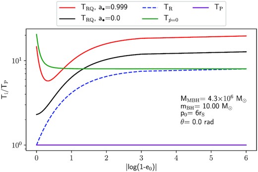
$Comparison between the different merger time-scales normalized to the Peters’ time-scale TP (purple solid line), for the case of a compact object of 10 M⊙ in an equatorial prograde orbit around a 4.3 × 106 M⊙ MBH, and a pericentre distance p0 = 6rS. The green solid line, $T_{\dot{p}=0}$, is the time-scale obtained with equation (3). The blue dashed line, TR, includes the correction for the secular eccentricity evolution R (equation 4). The black (a• = 0) and red (a• = 0.999) solid lines, TRQ, include the correction factors R and Q, which accounts for post-Newtonian effects up to order 1.5.$

Figure 1.

Comparison between the different merger time-scales normalized to the Peters’ time-scale T_P (purple solid line), for the case of a compact object of 10 M_⊙ in an equatorial prograde orbit around a 4.3 × 10⁶ M_⊙ MBH, and a pericentre distance p₀ = 6r_S. The green solid line, |$T_{\dot{p}=0}$|⁠, is the time-scale obtained with equation (3). The blue dashed line, T_R, includes the correction for the secular eccentricity evolution R (equation 4). The black (a_• = 0) and red (a_• = 0.999) solid lines, T_RQ, include the correction factors R and Q, which accounts for post-Newtonian effects up to order 1.5.

Open in new tab Download slide

Peters’ time-scale T_P underestimates the merger time since it assumes that the eccentricity remains at its initial value throughout the evolution, artificially boosting the radiation of GWs. In contrast, the time-scale |$T_{\dot{p}=0}$| overestimates the merger time-scale for low eccentricities since it assumes that the pericentre of the orbit does not decay, artificially decreasing the amount of GW emitted. The effect of the PN correction factors is to increase the estimate of the merger time-scale, especially for circular orbits. Nevertheless, for p₀ ≲ 6r_S and eccentricity values e₀ > 0.9, relevant for EMRIs and X-MRIs, |$T_{\dot{p}=0}\in (1.2 - 0.4)\times T_{\rm RQ}$|⁠. Table 1 summarizes the characteristics of the different merger time-scales.

Table 1.

Open in new tab

In this table, we summarize the characteristics and validity ranges of the different estimates for the GW-induced merger time-scales. We use the corrected time-scale T_RQ as a benchmark from which to say whether the time-scales |$T_{\dot{p}=0}$|⁠, T_P, and T_R over or underestimate the result.

Name	Validity	Time-scale accuracy	PN effects
T_P	Low e₀	Underestimates	No
\|$T_{\dot{p}=0}$\|	High e₀	Over/under	No
T_R	Any e₀	Underestimates	No
T_RQ	Any e₀	Best	Yes

Name	Validity	Time-scale accuracy	PN effects
T_P	Low e₀	Underestimates	No
\|$T_{\dot{p}=0}$\|	High e₀	Over/under	No
T_R	Any e₀	Underestimates	No
T_RQ	Any e₀	Best	Yes

Table 1.

Open in new tab

In this table, we summarize the characteristics and validity ranges of the different estimates for the GW-induced merger time-scales. We use the corrected time-scale T_RQ as a benchmark from which to say whether the time-scales |$T_{\dot{p}=0}$|⁠, T_P, and T_R over or underestimate the result.

Name	Validity	Time-scale accuracy	PN effects
T_P	Low e₀	Underestimates	No
\|$T_{\dot{p}=0}$\|	High e₀	Over/under	No
T_R	Any e₀	Underestimates	No
T_RQ	Any e₀	Best	Yes

Name	Validity	Time-scale accuracy	PN effects
T_P	Low e₀	Underestimates	No
\|$T_{\dot{p}=0}$\|	High e₀	Over/under	No
T_R	Any e₀	Underestimates	No
T_RQ	Any e₀	Best	Yes

3 THE CRITICAL SEMIMAJOR AXIS

The critical semimajor axis a_crit marks the end of the relaxation-driven evolution regime, i.e. two-body relaxation effects become irrelevant, and the energy loss due to GWs emission dominates the evolution of the orbit. Its value is found by solving

$$\begin{eqnarray*} T_{\rm GW}=T_{\rm peri}(a_0, e_0), \end{eqnarray*}$$

(6)

where T_GW is the merger time-scale, and T_peri is the time required by two-body relaxation to change the pericentre of the inspiraling object (Amaro-Seoane et al. 2007), given by

$$\begin{eqnarray*} T_{\rm peri}(a_0, e_0)=T_{\rm rlx}(a_0) \times \big(1-e_0^2\big). \end{eqnarray*}$$

(7)

This time-scale is derived from the angular momentum diffusion time-scale,

$$\begin{eqnarray*} T_{\rm J}\sim T_{\rm rlx} \times [J/J_{\rm max}]^2 =T_{\rm rlx}(a) \big(1-e_0^2\big), \end{eqnarray*}$$

(8)

where J = (a(1 − e²)GM_MBH)^1/2, J_max = (aGM_MBH)^1/2 is the angular momentum of a circular orbit, and T_rlx(a) is the relaxation time-scale at a distance equal to the semimajor axis a (see equation 12 below).

Two-body interactions also cause energy diffusion, which changes the semimajor axis of the objects orbiting the MBH on the relaxation time-scale

$$\begin{eqnarray*} T_{\rm rlx}\sim \mathcal {E}/\dot{ \mathcal {E}}, \end{eqnarray*}$$

(9)

where |$\mathcal {E}$| = GM_MBH/2a. This effect is not relevant to the inspiral process because, only by energy diffusion, it can take several relaxation time-scales to reach orbital parameters for which GWs emission becomes significant. From equation (8), if e₀ ≠ 0, then T_J ≲ T_rlx, indicating that two-body relaxation diffuses angular momentum faster than it diffuses energy (Hopman & Alexander 2005), increasing the eccentricity of an orbit while its semimajor axis remains approximately constant, allowing the object to reach very short distances to the MBH at the pericentre. This is a key dynamical aspect in the EMRIs/X-MRIs formation; taking T_peri(a₀, e₀) = T_J in equation (6) guarantees that objects with a₀ ≲ a_crit that reached highly eccentric orbits due to a decrease in their angular momentum, merge before their pericentre changes by diffusion. If the term |$(1-e_0^2)$| is omitted in the same equation, systems with longer T_GW for which diffusion in angular momentum is still significant can be mistakenly considered as potential inspiraling sources, artificially increasing the event rates.

At each pericentre passage, the energy loss by GWs emission is maximum, shrinking the semimajor axis and increasing the binding energy between the MBH and the compact object. If the new binding energy is high enough, the binary decouples dynamically from the surrounding stellar system, and diffusion in J and |$\mathcal {E}$| becomes negligible; the orbit then evolves only due to the energy loss by GWs emission, creating a successful inspiral that ends when the object crosses the event horizon of the central MBH. Otherwise, the object remains in the dynamical regime performing a random walk in the phase space driven by diffusion in energy and angular momentum, to either plunge into the MBH, diffuse to wider orbits, or become a potential inspiral source by diffusing into tighter orbits.

For each given semimajor axis a₀ ≲ a_crit, there is a critical eccentricity above which the orbiting compact object becomes immune to the relaxation processes and, by fixing the pericentre of the secondary body at the LSO around the MBH, we set a high-eccentricity limit given by e_plunge = 1 − r_LSO/a₀, where r_LSO is the position of the LSO. If, for a given a₀ ≲ a_crit, e₀ > e_plunge, the pericentre of the orbit is located inside the LSO and the orbiting body crosses the event horizon of the MBH, without inspiraling, after a single pericentre passage (Amaro-Seoane et al. 2007).

This formation scenario is characterized by the balance between T_peri and the GW time-scale T_GW. While the latter depends only on the source characteristics, the former requires a model of the stellar density in the vicinity of the MBH.

We obtain r_LSO from the critical angular momentum described in Teukolsky & Shapiro (1983) for a non-relativistic particle in a highly eccentric orbit around a Schwarzschild BH,

$$\begin{eqnarray*} J_{\rm crit}= 4GM_{\rm MBH}/c. \end{eqnarray*}$$

(10)

The above equation describes a parabolic orbit with a pericentre distance equal to p_LSO = 4r_S. As any particle with J < J_crit plunges into the MBH, the value of p_LSO defines the plunge radius. Therefore, for the Schwarzschild case, we assume that the LSO is located at the plunge radius r_LSO = 4r_S.

For a Kerr MBH, the change in the position of the LSO due to the spin and inclination with respect to the spin axis, is modelled through the function |$\mathcal {W} (\theta , a_{\bullet })$| derived in Amaro-Seoane et al. (2013) from the separatrices between stable and unstable (plunging) orbits. The inclusion of |$\mathcal {W} (\theta , a_{\bullet })$| can increase the number of cycles a prograde EMRI or X-MRI spends inside the LISA frequency band in such a way that it becomes detectable. Its derivation is based on the scheme presented in Sopuerta & Yunes (2011), that takes elements from the multipolar, post-Minkowskian formalism and BH perturbation theory to describe an inspiral trajectory, including also the radiation-reaction from the GWs emission to the system. For a Kerr MBH, the effective pericentre at the LSO is

$$\begin{eqnarray*} p = a(1-e) = \mathcal {W} (\theta , a_{\bullet }) \times \frac{8 G M_{\rm MBH}}{c^2}. \end{eqnarray*}$$

(11)

To estimate T_rlx, we consider that inside the influence radius of the MBH, defined as |$R_{\rm h}=GM_{\rm MBH}/\sigma _0^2$|⁠, with σ₀ the central velocity dispersion, the stellar density distribution follows a power-law cusp ρ(r) ∼ r^−γ. This is a theoretical prediction of Peebles (1972) and Bahcall & Wolf (1976) from the 1970s that has been tested in the past decade by numerical approaches (see, e.g. Freitag & Benz 2001; Amaro-Seoane, Freitag & Spurzem 2004; Preto & Amaro-Seoane 2009), concluding that stellar cusps may be common around MBHs. A strong support of these assumptions is found in the work of Gallego-Cano et al. (2018), Schödel et al. (2018), Baumgardt, Amaro-Seoane & Schödel (2018), in which the authors conduct an extensive search for the stellar density cusp around Sgr A*, by performing observations and N-body simulations of the innermost structure of the Milky Way’s nuclear star cluster. They find an excellent agreement between the theory, their observational data, and their simulations, consistent with the existence of a power-law density cusp around Sgr A*.

Stellar-mass BHs dominate the central density as they sink to the centre due to mass segregation forming a cusp for which different indices have been suggested, for example γ = 1.3–1.4 (Freitag, Amaro-Seoane & Kalogera 2006), γ = 1.75 (Bahcall & Wolf 1976), and 2 ≲ γ ≲ 11/4 in strong mass segregation scenarios (Alexander & Hopman 2009; Preto & Amaro-Seoane 2009; Amaro-Seoane & Preto 2011). We assume that these objects with a typical mass of m_BH = 10 M_⊙ are the driving species in the relaxation process. Less massive species distribute into a shallower profile and do not affect the relaxation rates.

The relaxation time-scale inside R_h at a distance equal to the semimajor axis a (Baumgardt, Makino & Ebisuzaki 2004a, b; Freitag & Benz 2002; Hopman & Alexander 2005) is

$$\begin{eqnarray*} T_{\rm rlx} = T_0\left(\frac{a}{R_{\rm h}}\right)^{\gamma -3/2}, \end{eqnarray*}$$

(12)

$$\begin{eqnarray*} T_0=0.3389\, \frac{\sigma ^3_0}{\text{ln}(\Lambda) G^2 m_{\rm BH}^2 n_0 }, \end{eqnarray*}$$

(13)

where ln(Λ) ≃ 13 is the Coulomb logarithm (Binney & Tremaine 1987), and n₀ is the number density given by

$$\begin{eqnarray*} n_0 = \frac{3-\gamma }{4\pi }\frac{N_0}{R^3_{\rm h}}, \end{eqnarray*}$$

(14)

$$\begin{eqnarray*} \sigma _0 =\left(\frac{1}{1+\gamma }\frac{G M_{\rm MBH}}{R_{\rm h}} \right)^{1/2}, \end{eqnarray*}$$

(15)

where N₀ is the number of stellar-mass BHs inside R_h. With these elements, equation (13) becomes

$$\begin{eqnarray*} T_0 \simeq \frac{4.26}{(3-\gamma)(1+\gamma)^{3/2}} \frac{\sqrt{R_{\rm h}^{3}(GM_{\rm MBH})^{-1}}}{\text{ln}(\Lambda) N_0}\left(\frac{M_{\rm MBH}}{m_{\rm BH}} \right)^2. \end{eqnarray*}$$

(16)

As inspiral time-scale, we take equation (5) to include the correction factors, and evaluate it at the LSO as long as it is located no closer than 3r_S. At shorter distances, the correction factors involving the PN terms are not accurate (Zwick et al. 2021); in that case, we compute Q at 3r_S. We re-write the correction factor Q in terms of the MBH spin, the function |$\mathcal {W} (\theta ,a_{\bullet })$|⁠, and the initial eccentricity.

If p₀ ≤ 3r_S, the correction factor Q is computed at 3r_S:

$$\begin{eqnarray*} Q &= &\exp (A) \left[1.67-2.75\left(e_0^2-3.16e_0\right)\right], \nonumber \\ A &=& s\left[\frac{0.15}{1.5} e_0 + 1.37(1-e_0)^{3/2}\right] \nonumber \\ &&+\,|s|^{3/2} \left[\left(0.36 e_0\right)^{5/2} + 2.94(1-e_0)^3\right], \end{eqnarray*}$$

(17)

where s = a_•cos (θ).

If p₀ > 3r_S, the correction factor Q is given by

$$\begin{eqnarray*} Q=q_{\rm h}\left(e_0,\mathcal {W}(\theta ,a_{\bullet })\right)q_{\rm s}\left(s,e_0,\mathcal {W} (\theta , a_{\bullet })\right), \end{eqnarray*}$$

(18)

with

$$\begin{eqnarray*} q_{\rm h}(e_0,\mathcal {W}(\theta ,a_{\bullet })) &=& \exp \Big (\frac{0.7}{\mathcal {W}(\theta ,a_{\bullet })}\Big) \times \Bigg \lbrace 1+ (1-e_0)^2 \nonumber\\ &&\times \,\left[\exp \left(\frac{0.55}{\mathcal {W}(\theta ,a_{\bullet })}\right)-1\Big)\right] \nonumber \\ &&+\,\left(\frac{0.95}{\mathcal {W}(\theta ,a_{\bullet })}\right)^{3/2}\left(e_0^2-e_0\right)\Bigg \rbrace ,\nonumber \end{eqnarray*}$$

$$\begin{eqnarray*} q_{\rm s}\left(s,e_0,\mathcal {W}(\theta ,a_{\bullet })\right) &=& \exp \Bigg \lbrace s \Bigg [ \frac{0.3 \, e_0}{4\mathcal {W} (\theta , a_{\bullet })} + \left(1-e_0\right)^{3/2}\nonumber\\ && \times \left(\!\frac{3.7}{4\mathcal {W} (\theta , a_{\bullet })}\! \right)^{3/2}\Bigg ]\!+\! |s|^{3/2} \Bigg [\!\!\left(\!\frac{0.275 \, e_0}{\mathcal {W} (\theta , a_{\bullet })} \right)^{5/2} \nonumber \\ &&+\,(1-e_0)^3\left(\frac{1.075}{\mathcal {W} (\theta , a_{\bullet })} \right)^3\Bigg ] \Bigg \rbrace . \end{eqnarray*}$$

Combining these elements, the critical semimajor axis takes the form

$$\begin{eqnarray*} a_{\rm crit} &=& R_{\rm h} \left[\varepsilon \,\, \mathcal {W}(\theta , a_{\bullet })^{5/2} \frac{m_{\rm BH}^2}{m_2(M_{\rm MBH} + m_2)}\right] ^{1/(\gamma - 3)} \nonumber \\ &&\times \left[\frac{f(e_0)}{\big(1-e_0^2\big)(1-e_0)^{5/2}}\,\, R\, Q\right]^{1/(\gamma - 3)}, \nonumber \\ \varepsilon &=& \frac{(3-\gamma)(1+\gamma)^{3/2}}{4.26} \left(\frac{5\times 8^{5/2}}{256}\right)N_0 \text{ln}(\Lambda). \end{eqnarray*}$$

(19)

The correction factors can be turned off by setting RQ = 1, in which case a_crit is determined by T_P (equation 1) and is denoted as a_P. If the correction factors RQ are applied, the critical semimajor axis is denoted as a_RQ, and as |$a_{\dot{p}=0}$| if its value is derived using |$T_{\dot{p}=0}$| as the merger time-scale (see equation 28 in Amaro-Seoane 2019).

Fig. 2 shows the values of a_RQ, a_P, and |$a_{\dot{p}=0}$| for a BD X-MRI with e₀ = 0.998 inspiraling into a Schwarzschild MBH, and into a Kerr MBH for which a_• = 0.999, and θ = 0.1 rad. For a_• = 0, we find that a_P ∼ 8.5 a_RQ, which can significantly reduce the event rates when computed with a_RQ; in contrast, the value of |$a_{\dot{p}=0}$| is of about 0.9 a_RQ. In the Kerr case, the effect of R and Q is larger resulting in a_P ∼ 12 a_RQ, and |$a_{\dot{p}=0}\sim 1.3 ~a_{\rm RQ}$|⁠.

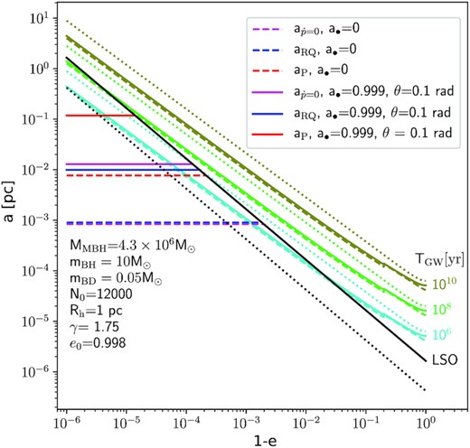
$Critical semimajor axis as a function of eccentricity, for an inspiraling BD with e0 = 0.998. We consider a• = 0 and a• = 0.999, for which the orbital inclination of the BD is θ=0.1 rad. These values of spin and θ maximize the correction associated with the spin. The diagonal green coloured curves are isochrones that represent the inspiral time of the binary in years. The dotted isochrones are obtained with Peters’ formula (equation 1), the solid isochrones with the corrected time-scale TRQ and a• = 0, and the dashed isochrones with TRQ and a• = 0.999. Black lines represent the LSO, the solid line is the Schwarzschild case, and the dotted, the Kerr case. The intersection between the LSO and the horizontal lines are the values of acrit for the Schwarzschild and Kerr cases. The subscript RQ (blue lines) indicates that the correction factors in equation (19) are included, whereas the subscript P (red lines) indicates the value without the corrections. The magenta lines indicates the value of $a_{\dot{p}=0}$, obtained using the merger time-scale $T_{\dot{p}=0}$, given by equation (3).$

Figure 2.

Critical semimajor axis as a function of eccentricity, for an inspiraling BD with e₀ = 0.998. We consider a_• = 0 and a_• = 0.999, for which the orbital inclination of the BD is θ=0.1 rad. These values of spin and θ maximize the correction associated with the spin. The diagonal green coloured curves are isochrones that represent the inspiral time of the binary in years. The dotted isochrones are obtained with Peters’ formula (equation 1), the solid isochrones with the corrected time-scale T_RQ and a_• = 0, and the dashed isochrones with T_RQ and a_• = 0.999. Black lines represent the LSO, the solid line is the Schwarzschild case, and the dotted, the Kerr case. The intersection between the LSO and the horizontal lines are the values of a_crit for the Schwarzschild and Kerr cases. The subscript RQ (blue lines) indicates that the correction factors in equation (19) are included, whereas the subscript P (red lines) indicates the value without the corrections. The magenta lines indicates the value of |$a_{\dot{p}=0}$|⁠, obtained using the merger time-scale |$T_{\dot{p}=0}$|⁠, given by equation (3).

Open in new tab Download slide

The difference between a_P and the values obtained for |$a_{\dot{p}=0}$| and a_RQ originates in the lack of accuracy of Peters’ time-scale for highly eccentric and relativistic orbits, revealing the need to thoroughly verify Peters’ time-scale’s validity depending on the physical characteristics of the system.

4 THE INSPIRAL EVENT RATE

The event rate of successful inspirals is calculated by integrating the number of sources (Hopman & Alexander 2005), n(a), in a volume defined from the minimum distance at which we expect to find at least one potential EMRI/X-MRI source, a_min (Amaro-Seoane 2019, see equation 23 below), to the critical semimajor axis:

$$\begin{eqnarray*} \dot{\Gamma }_{\rm i} \simeq \int _{a_{\rm min}}^{a_{\rm crit}} \frac{{\rm d}n(a)}{T_{\rm rlx} (a)\,\, \text{ln}(\widehat{\theta }_{\rm lc}^{-2})}, \end{eqnarray*}$$

(20)

where dn(a) is obtained from the number of potential sources around the MBH, as explained below, and |$\widehat{\theta }_{\rm lc}$| is the loss-cone angle associated to the position of the LSO.

Inside the integration volume defined by a_min and a_crit, two-body relaxation is the leading mechanism that brings a source sufficiently close to the MBH to produce an inspiral event. In the following section, we derive a_min, dn(a), and the loss-cone angle of a Kerr MBH that can deviate from a Schwarzschild loss-cone angle if the spin of the MBH is sufficiently high.

4.1 Number of sources around an MBH

To obtain the number of objects of a given species, we assume that, similarly to stellar-mass BHs, lighter objects follow a mass density distribution given by a power law with exponent β, resulting in a two-population system in which the value of γ dictates the distribution of the stellar-mass BHs around the MBH, and β the inspiraling object’s population distribution. The number of objects of a given species within a given semimajor axis is

$$\begin{eqnarray*} N(a)=f_{\rm sub} N_{\rm tot} \left(\frac{a}{R_{\rm h}}\right)^{3-\beta }, \end{eqnarray*}$$

(21)

where N_tot is the total number of objects (main-sequence stars, compact objects, and substellar objects) within the influence radius of the MBH, and f_sub is the fraction number of the considered species obtained from a Kroupa (2001) broken power law, |$\Phi (m)\propto m_{\ast }^{-\alpha }$|⁠, with m_⋆ the average stellar mass. We use α = [0.3, 1.3, 2.3] for the mass intervals [0.01, 0.07, 0.5, 150] × M_⊙ where [0.01–0.07] M_⊙ is the BD mass range. Table 2 shows the masses and fraction numbers of each considered object. The numerator of equation (20) comes from differentiating equation (21)

$$\begin{eqnarray*} {\rm d}n(a)= f_{\rm sub}(3-\beta) \frac{N_{\rm tot}}{R_{\rm h}} \left(\frac{a}{R_{\rm h}}\right)^{2-\beta } da. \end{eqnarray*}$$

(22)

The distance a_min at which at least one object of a given species can be found is obtained by setting equation (21) equal to 1 and taking N_tot = M_MBH/m_⋆,

$$\begin{eqnarray*} a_{\rm min}=R_{\rm h}\left(\frac{m_{\star }}{f_{\rm sub} \, M_{\rm MBH}} \right)^{1/(3-\beta)}. \end{eqnarray*}$$

(23)

Table 2.

Open in new tab

Mass and fraction number of inspiraling objects.

Inspiraling object	mass [M_⊙]	f_sub
Stellar-mass BH	10.0	8.13 × 10⁻⁴
Neutron star (NS)	2.7	4.24 × 10⁻³
White dwarf (WD)	0.8	7.20 × 10⁻²
Brown dwarf (BD)	0.05	0.21

Inspiraling object	mass [M_⊙]	f_sub
Stellar-mass BH	10.0	8.13 × 10⁻⁴
Neutron star (NS)	2.7	4.24 × 10⁻³
White dwarf (WD)	0.8	7.20 × 10⁻²
Brown dwarf (BD)	0.05	0.21

Table 2.

Open in new tab

Mass and fraction number of inspiraling objects.

Inspiraling object	mass [M_⊙]	f_sub
Stellar-mass BH	10.0	8.13 × 10⁻⁴
Neutron star (NS)	2.7	4.24 × 10⁻³
White dwarf (WD)	0.8	7.20 × 10⁻²
Brown dwarf (BD)	0.05	0.21

Inspiraling object	mass [M_⊙]	f_sub
Stellar-mass BH	10.0	8.13 × 10⁻⁴
Neutron star (NS)	2.7	4.24 × 10⁻³
White dwarf (WD)	0.8	7.20 × 10⁻²
Brown dwarf (BD)	0.05	0.21

4.2 The loss-cone angle for Schwarzschild and Kerr black holes

Not all the objects that approach the MBH can produce an EMRI or X-MRI. The pericentre distance has to be sufficiently small for GWs emission to occur; however, if it falls within the LSO, the object suffers a direct plunge. We can identify plunging orbits through their velocity vector; if it lies within a cone defined by a half-angle equal to the loss-cone angle, the orbit takes the object inside a sphere of radius equal to the LSO and rapidly merges with the MBH. The loss-cone angle is calculated as

$$\begin{eqnarray*} \widehat{\theta }_{\rm lc}=\left(\frac{J_{\rm max}}{J_{\rm lc}}\right)^{-1/2}, \end{eqnarray*}$$

(24)

where |$J_{\rm lc}^2$| is the angular momentum of an orbit around the MBH that takes a particle to a distance equal to the loss-cone radius r_lc. For a Schwarzschild BH, we take J_lc = J_crit from equation (10), so that r_{lc, S} = 4r_S, thus the associated loss-cone angle is

$$\begin{eqnarray*} \widehat{\theta }_{\rm S}=\left(\frac{a}{8 r_{\rm S}}\right)^{-1/4}. \end{eqnarray*}$$

(25)

For a Kerr BH, the shift in the LSO changes the loss-cone radius; therefore, it is necessary to implement a Kerr loss-cone angle that considers this effect. We implement two versions for the Kerr loss-cone angle; the first, is based on the LSO position shift given by the function |$\mathcal {W}$| (θ, a_•). We write the Kerr loss-cone radius as |$r_{\rm lc,\mathcal {W}} = 4 r_{\rm S} \mathcal {W}$| (θ, a_•); the associated loss-cone angle is

$$\begin{eqnarray*} \widehat{\theta }_{\mathcal {W}}=\left(\frac{a}{8 r_{\rm S} \mathcal {W}(\theta , a_{\bullet })}\right)^{-1/4}= \widehat{\theta }_{\rm S}\mathcal {W}(\theta , a_{\bullet })^{1/4} \end{eqnarray*}$$

(26)

For the second version, we use the analytic approximation for the critical angular momentum (J_crit) of a non-relativistic test particle orbiting a Kerr BH obtained by Will (2012), which compared to numerical solutions is accurate within a 5 per cent for 0.9 ≤ a_• ≤ 0.99, and is valid for arbitrary orbital inclinations:

$$\begin{eqnarray*} J_{\rm crit} &= &\frac{GM}{c}\left[2 K(\theta ,a_{\bullet})+ 2 \right], \nonumber \\ K(\theta ,a_{\bullet }) &=& \sqrt{1-s-(1/8)a_{\bullet }^2\sin ^2(\theta) F(a_{\bullet },\cos (\theta)}), \nonumber \\ F(a_{\bullet },\cos (\theta)) &=& 1+\frac{s}{2}+\frac{a_{\bullet }^2}{64}(7 + 13 \cos ^2(\theta)) \nonumber \\ &&+\,\frac{a_{\bullet }^2s}{128} (23 + 5 \cos ^2(\theta)) + \frac{a_{\bullet }^4}{2048} \nonumber \\ &&\times \, (55 + 340 \cos ^2(\theta) - 59 \cos ^4(\theta)) + \mathcal {O}^5(a_{\bullet }^5). \nonumber\\ \end{eqnarray*}$$

(27)

A particle with J < J_crit rapidly plunges into the MBH, determining a Kerr loss-cone angle given by

$$\begin{eqnarray*} \widehat{\theta }_{\rm K}=\left(\frac{2 a}{r_{\rm S}}\left[2K(\theta ,a_{\bullet }) +2\right]^{-2}\right)^{-1/4}. \end{eqnarray*}$$

(28)

An inspiraling object approaching an MBH in a prograde orbit finds the LSO closer to the MBH; consequently, the loss-cone angle magnitude decreases with respect to the Schwarzschild case, and it is easier for the incoming body to avoid direct plunge. For retrograde orbits, the LSO is pushed away from the MBH; hence the loss-cone angle magnitude is larger than in the prograde cases, increasing the phase space that produces a direct plunge. This effect can be easily seen in equation (26) as |$\mathcal {W} (\theta , a_{\bullet }) \lesssim 1$| for prograde orbits, and ≳1 for the retrograde cases.

In Fig. 3, we show that the two versions of the Kerr loss-cone angle yield similar results, especially for retrograde orbits with θ ≲ −1.3 rad. The value of |$\widehat{\theta }_{\rm K}$| slightly deviates from |$\widehat{\theta }_{\rm \mathcal {W}}$| in the case of prograde orbits with θ ∼ 0.4–0.7 rad and a_• ≳ 0.95.

$The figure shows the ratio between the loss-cone angles $\widehat{\theta }_{\rm i}/ \widehat{\theta }_{\rm j}=[\widehat{\theta }_{\rm \mathcal {W}}/\widehat{\theta }_{\rm S}, ~\widehat{\theta }_{\rm K}/ \widehat{\theta }_{\rm S},~\widehat{\theta }_{\rm K}/\widehat{\theta }_{\rm \mathcal {W}}]$ obtained with equations (25), (26) and (28). We show prograde (top panel) and retrograde (bottom panel) orbits with three different orbital inclinations: |θ| = [0.1, 0.7, 1.57] rad. The black horizontal line is plotted as a reference: the closer the lines are to the black line, the closer the values are between them. The ratios $\widehat{\theta }_{\rm \mathcal {W}}/\widehat{\theta }_{\rm S}$ and $\widehat{\theta }_{\rm K}/ \widehat{\theta }_{\rm S}$ indicate the deviation of the Kerr loss-cone angle with respect to the Schwarzschild case as a function of the MBH spin, whereas $\widehat{\theta }_{\rm K}/\widehat{\theta }_{\rm \mathcal {W}}$ shows the difference between the two versions of the Kerr loss-cone angle.$

Figure 3.

The figure shows the ratio between the loss-cone angles |$\widehat{\theta }_{\rm i}/ \widehat{\theta }_{\rm j}=[\widehat{\theta }_{\rm \mathcal {W}}/\widehat{\theta }_{\rm S}, ~\widehat{\theta }_{\rm K}/ \widehat{\theta }_{\rm S},~\widehat{\theta }_{\rm K}/\widehat{\theta }_{\rm \mathcal {W}}]$| obtained with equations (25), (26) and (28). We show prograde (top panel) and retrograde (bottom panel) orbits with three different orbital inclinations: |θ| = [0.1, 0.7, 1.57] rad. The black horizontal line is plotted as a reference: the closer the lines are to the black line, the closer the values are between them. The ratios |$\widehat{\theta }_{\rm \mathcal {W}}/\widehat{\theta }_{\rm S}$| and |$\widehat{\theta }_{\rm K}/ \widehat{\theta }_{\rm S}$| indicate the deviation of the Kerr loss-cone angle with respect to the Schwarzschild case as a function of the MBH spin, whereas |$\widehat{\theta }_{\rm K}/\widehat{\theta }_{\rm \mathcal {W}}$| shows the difference between the two versions of the Kerr loss-cone angle.

Open in new tab Download slide

The MBH spin effects are weak for θ ∼ ±1.57 rad, and both versions of the Kerr loss-cone angle indicates that if the inspiraling object approaches an MBH in a highly inclined orbit, regardless if it is in a prograde or retrograde orbit, the phase space that produces a direct plunge is reduced if the MBH is rotating. The strongest spin effects appear with θ = ±0.1 rad and a_• = 0.999; in the case of prograde orbits, |$\widehat{\theta }_{\rm \mathcal {W}} \sim \widehat{\theta }_{\rm K} \sim 0.5 \, \widehat{\theta }_{\rm S}$|⁠, and |$\widehat{\theta }_{\rm \mathcal {W}} \sim \widehat{\theta }_{\rm K} \sim 1.19 \, \widehat{\theta }_{\rm S}$| for θ = −0.1 rad.

Finally, we use equations (12), (22) and (24) to solve equation (20) with the correction factors embedded in the value of a_crit, thus obtaining

$$\begin{eqnarray*} \dot{\Gamma }_{\rm i} &=& \frac{3-\beta }{2\lambda T_0} \,\,\frac{ N_{tot}}{R_h^{\lambda }}\,\, f_{\rm sub} \left\lbrace \left[ a_{\rm crit}^{\lambda }\left(\text{ln}\left(\frac{a_{\rm crit}}{D}\right)- \frac{1}{\lambda }\right)\right]\right. \nonumber\\ &&\left.-\, \left[ a_{\rm min}^{\lambda } \left(\text{ln}\left(\frac{a_{\rm min}}{D}\right)- \frac{1}{\lambda } \right) \right] \right\rbrace , \end{eqnarray*}$$

(29)

with λ = (9/2) − β − γ, and D a term associated to the loss-cone angle, given by

$$\begin{eqnarray*} D= \left\lbrace \begin{array}{@{}l@{\quad }l@{}}8 r_{\rm S}, & \text{for}\ \widehat{\theta }_{\rm lc}^{-2}=\widehat{\theta }_{\rm S}^{-2},\\ 8 r_{\rm S} \mathcal {W}(\theta ,\rm a_{\bullet }), &\text{for}\ \widehat{\theta }_{\rm lc}^{-2}=\widehat{\theta }_{\mathcal {W}}^{-2},\\ 0.5 r_{\rm S} \left[2 + 2 K(\theta ,a_{\bullet })\right]^2,& \text{for}\ \widehat{\theta }_{\rm lc}^{-2}=\theta ^{-2}_{\rm K}. \end{array}\right. \end{eqnarray*}$$

(30)

5 EFFECT OF THE CORRECTION FACTORS AND THE LOSS-CONE ANGLE IN THE EVENT RATES

Applying the correction factors results in longer merger time-scales compared to T_P and |$T_{\dot{p}=0}$| (for high enough eccentricities), giving more time to the relaxation processes to perturb the orbit of the compact object and prevent an inspiral. Therefore, to decouple from the dynamics regime, the inspiraling body has to be closer to the MBH, resulting in a smaller critical semimajor axis such that |$a_{\rm RQ} \lesssim a_{\dot{p}=0}\lt a_{\rm P}$|⁠. The semimajor axis a₀ of an inspiraling object would be delimited by a_min and a_crit < R_h, and the pericentre distance would be fixed at the LSO position (equation 11). With these conditions, we define an eccentricity range e₀ = [e_min(a_•, θ), e_max(a_•, θ)] given by

$$\begin{eqnarray*} &e_{\rm max}(a_{\bullet },{\theta })= 1-r_{\rm LSO}/a_{\rm crit}, \end{eqnarray*}$$

(31)

$$\begin{eqnarray*} &e_{\rm min}(a_{\bullet },{\theta })= 1-r_{\rm LSO}/a_{\rm min}. \end{eqnarray*}$$

(32)

Objects with e₀ > e_max plunge into the MBH after a single pericentre passage, and as we do not expect to find objects with a₀ < a_min, the value of e_min defines the plunging limit for the objects that are located closest to the MBH.

As the pericentre is fixed, orbits with |$a_0=a_{\dot{p}=0}$|⁠, and specially with a₀ = a_P can have higher eccentricities than orbits with a₀ = a_RQ. For this reason, we obtain e_max by setting a_crit = a_RQ in equation (31); this eccentricity value is valid for all the cases, as a_crit sets the upper limit for the semimajor axis of an inspiraling orbit. Table 3 shows the range of eccentricities for the considered compact objects obtained for θ = ±0.1 rad, a_• = [0.0, 0.999], and a_crit = a_RQ.

Table 3.

Open in new tab

Maximum and minimum eccentricity (equations 31 and 32) for each type of compact object. The values of e_min and e_max are obtained for θ = 0.1 rad (prograde orbits), θ = −0.1 rad (retrograde orbits), a_crit = a_RQ, M_MBH = 4.3 × 10⁶ M_⊙, and a_• = 0 or 0.999.

a_• = 0.0
Object	e_min		e_max
BD	0.963178		0.998160
WD	0.981957		0.999790
NS	0.997268		0.999919
BH	0.996791		0.999971
a_• = 0.999
	Prograde		Retrograde
	e_min	e_max	e_min	e_max
BD	0.990605	0.999954	0.947489	0.995773
WD	0.995396	0.999995	0.974270	0.999505
NS	0.999303	0.999998	0.996104	0.999810
BH	0.999181	0.999999	0.995424	0.999932

a_• = 0.0
Object	e_min		e_max
BD	0.963178		0.998160
WD	0.981957		0.999790
NS	0.997268		0.999919
BH	0.996791		0.999971
a_• = 0.999
	Prograde		Retrograde
	e_min	e_max	e_min	e_max
BD	0.990605	0.999954	0.947489	0.995773
WD	0.995396	0.999995	0.974270	0.999505
NS	0.999303	0.999998	0.996104	0.999810
BH	0.999181	0.999999	0.995424	0.999932

Table 3.

Open in new tab

Maximum and minimum eccentricity (equations 31 and 32) for each type of compact object. The values of e_min and e_max are obtained for θ = 0.1 rad (prograde orbits), θ = −0.1 rad (retrograde orbits), a_crit = a_RQ, M_MBH = 4.3 × 10⁶ M_⊙, and a_• = 0 or 0.999.

a_• = 0.0
Object	e_min		e_max
BD	0.963178		0.998160
WD	0.981957		0.999790
NS	0.997268		0.999919
BH	0.996791		0.999971
a_• = 0.999
	Prograde		Retrograde
	e_min	e_max	e_min	e_max
BD	0.990605	0.999954	0.947489	0.995773
WD	0.995396	0.999995	0.974270	0.999505
NS	0.999303	0.999998	0.996104	0.999810
BH	0.999181	0.999999	0.995424	0.999932

a_• = 0.0
Object	e_min		e_max
BD	0.963178		0.998160
WD	0.981957		0.999790
NS	0.997268		0.999919
BH	0.996791		0.999971
a_• = 0.999
	Prograde		Retrograde
	e_min	e_max	e_min	e_max
BD	0.990605	0.999954	0.947489	0.995773
WD	0.995396	0.999995	0.974270	0.999505
NS	0.999303	0.999998	0.996104	0.999810
BH	0.999181	0.999999	0.995424	0.999932

For the mass density distribution, we choose γ = 1.75 for the stellar-mass BHs, β = 1.5 for the lighter populations (Bahcall & Wolf 1976), R_h = 1 pc, and N₀ = 1.2 × 10⁴. We focus on systems composed of a central MBH of 4.3 × 10⁶ M_⊙ with a spin range a_• = [0.0–0.999] and an inspiraling object (a stellar-mass BH, an NS or a WD in the case of EMRIs; a BD in the case of X-MRIs) of mass m₂; the masses and fraction numbers are given in Table 2. Although we focus on MBHs of mass 4.3 × 10⁶ M_⊙, we include event-rate estimates for BH EMRIs with a central MBH of mass ranging from 10⁴ to 10⁷ M_⊙, which can be relevant for LISA.

5.1 The effect of the correction factors

To investigate the effect of the correction factors in the inspiraling rates, we estimate |$\dot{\Gamma }_{\rm i}$| with |$\widehat{\theta }_{\rm lc}=\widehat{\theta }_{\rm S}$| in the eccentricity range given by equations (31) and (32). We denote as |$\dot{\Gamma }_{\rm P}$| the event rates without the corrections, i.e. setting RQ = 1 in equation (29), as |$\dot{\Gamma }_{\rm RQ}$| the rates with the correction factors included, and as |$\dot{\Gamma }_{\dot{p}=0}$| the event rates computed as in Amaro-Seoane et al. (2013), where equation (3) is used as merger time-scale.

For the initial eccentricities given in Table 3, the correction factor R (equation 4) takes a value that goes from R ∼ 5 when e₀ ∼ 0.94, to ∼8 when e → 1. The factor Q (equations 17 and 18) is mainly affected by the spin and the orbital inclination; for a fixed θ, the PN correction reaches its maximum value when a_• = 0.999.

Figs 4 and 5 show the ratios |$\dot{\Gamma }_{\rm P}/\dot{\Gamma }_{\rm RQ}$| and |$\dot{\Gamma }_{\rm P}/\dot{\Gamma }_{\dot{p}=0}$|⁠, respectively, as a function of the initial eccentricity for the considered EMRIs and X-MRIs in prograde and retrograde orbits with θ = ±0.1 rad, |$\widehat{\theta }_{\rm lc}=\widehat{\theta }_{\rm S}$|⁠, and a_• = 0.999. These plots show the largest difference between the rates, as this configuration of MBH spin and orbital inclinations results in the highest (lowest) event rates in the case of prograde (retrograde) orbits. As shown in Table 4, the combined effect of the eccentricity evolution and the PN corrections represents an important improvement over |$\dot{\Gamma }_{\rm P}$|⁠: for a central MBH with a_• = 0.999, |$\dot{\Gamma }_{\rm P}\sim 8 - 30~ \dot{\Gamma }_{\rm RQ}$|⁠; for a_• = 0, |$\dot{\Gamma }_{\rm P}\sim 10 - 20 ~\dot{\Gamma }_{\rm RQ}$|⁠. On the other hand, the estimate given by |$\dot{\Gamma }_{\dot{p}=0}$| is between ∼1.3 and 2 times larger than the fully corrected value |$\dot{\Gamma }_{\rm RQ}$| when a_• = 0, and between |$\dot{\Gamma }_{\dot{p}=0} \sim 0.9 - 3 ~\dot{\Gamma }_{\rm RQ}$| for a_• = 0.999.

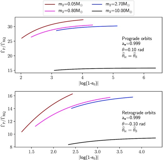
$Ratio $\dot{\Gamma }_{\rm P}/ \dot{\Gamma }_{\rm RQ}$ as a function of the initial eccentricity for EMRIs and X-MRIs in orbits with θ = 0.1 rad (upper panel) and θ = −0.1 rad (lower panel) around a 4.3 × 106 M⊙ Kerr MBH with a• = 0.999. $\dot{\Gamma }_{\rm P}$ represents the event rates obtained using Peters’ formula as the merger time-scale (i.e. setting RQ = 1 in equation 29), whereas $\dot{\Gamma }_{\rm RQ}$ are the corrected values. Both event rates are obtained with the usual loss-cone angle $\widehat{\theta }_{\rm S}$. Brown lines represent a BD (m2 = 0.05 M⊙) X-MRI, blue lines an inspiraling NS (m2 = 2.7 M⊙) EMRI, pink lines a WD (m2 = 0.8 M⊙) EMRI, and black lines a stellar-mass BH (m2 = 10 M⊙) EMRI.$

Figure 4.

Ratio |$\dot{\Gamma }_{\rm P}/ \dot{\Gamma }_{\rm RQ}$| as a function of the initial eccentricity for EMRIs and X-MRIs in orbits with θ = 0.1 rad (upper panel) and θ = −0.1 rad (lower panel) around a 4.3 × 10⁶ M_⊙ Kerr MBH with a_• = 0.999. |$\dot{\Gamma }_{\rm P}$| represents the event rates obtained using Peters’ formula as the merger time-scale (i.e. setting RQ = 1 in equation 29), whereas |$\dot{\Gamma }_{\rm RQ}$| are the corrected values. Both event rates are obtained with the usual loss-cone angle |$\widehat{\theta }_{\rm S}$|⁠. Brown lines represent a BD (m₂ = 0.05 M_⊙) X-MRI, blue lines an inspiraling NS (m₂ = 2.7 M_⊙) EMRI, pink lines a WD (m₂ = 0.8 M_⊙) EMRI, and black lines a stellar-mass BH (m₂ = 10 M_⊙) EMRI.

Open in new tab Download slide

$Same as Fig. 4, but for the ratio $\dot{\Gamma }_{\dot{p}=0} / \dot{\Gamma }_{\rm RQ}$. The rates $\dot{\Gamma }_{\dot{p}=0}$ are obtained using equation (3) as the merger time-scale.$

Figure 5.

Same as Fig. 4, but for the ratio |$\dot{\Gamma }_{\dot{p}=0} / \dot{\Gamma }_{\rm RQ}$|⁠. The rates |$\dot{\Gamma }_{\dot{p}=0}$| are obtained using equation (3) as the merger time-scale.

Open in new tab Download slide

Table 4.

Open in new tab

Ratios |$\dot{\Gamma }_{\rm P}/ \dot{\Gamma }_{\rm RQ}$| and |$\dot{\Gamma }_{\dot{p}=0}/ \dot{\Gamma }_{\rm RQ}$| for EMRIs and X-MRIs with θ = ±0.1 rad, around an MBH of mass M_MBH = 4.3 × 10⁶ M_⊙, and a_• = 0 or 0.999.

a_• = 0.0	\|$\dot{\Gamma }_{\rm P} / \dot{\Gamma }_{\rm RQ}$\|		\|$\dot{\Gamma }_{\dot{p}=0}/ \dot{\Gamma }_{\rm RQ}$\|
	e_min	e_max	e_min	e_max
BD	14.429	21.712	1.364	2.057
WD	15.319	20.628	1.566	2.110
NS	18.360	20.408	1.913	2.127
BH	10.436	11.500	1.675	1.846
a_• = 0.999	\|$\dot{\Gamma }_{\rm P} / \dot{\Gamma }_{\rm RQ}$\|
	θ = 0.1 rad		θ = −0.1 rad
	e_min	e_max	e_min	e_max
BD	26.021	32.344	10.365	16.295
WD	26.396	30.533	11.234	15.751
NS	28.609	30.205	14.031	15.794
BH	14.990	15.788	8.366	9.396
a_• = 0.999	\|$\dot{\Gamma }_{\dot{p}=0}/ \dot{\Gamma }_{\rm RQ}$\|
	θ = 0.1 rad		θ = −0.1 rad
	e_min	e_max	e_min	e_max
BD	2.693	3.349	0.936	1.477
WD	2.838	3.283	1.125	1.579
NS	3.114	3.288	1.433	1.614
BH	2.496	2.629	1.323	1.486

a_• = 0.0	\|$\dot{\Gamma }_{\rm P} / \dot{\Gamma }_{\rm RQ}$\|		\|$\dot{\Gamma }_{\dot{p}=0}/ \dot{\Gamma }_{\rm RQ}$\|
	e_min	e_max	e_min	e_max
BD	14.429	21.712	1.364	2.057
WD	15.319	20.628	1.566	2.110
NS	18.360	20.408	1.913	2.127
BH	10.436	11.500	1.675	1.846
a_• = 0.999	\|$\dot{\Gamma }_{\rm P} / \dot{\Gamma }_{\rm RQ}$\|
	θ = 0.1 rad		θ = −0.1 rad
	e_min	e_max	e_min	e_max
BD	26.021	32.344	10.365	16.295
WD	26.396	30.533	11.234	15.751
NS	28.609	30.205	14.031	15.794
BH	14.990	15.788	8.366	9.396
a_• = 0.999	\|$\dot{\Gamma }_{\dot{p}=0}/ \dot{\Gamma }_{\rm RQ}$\|
	θ = 0.1 rad		θ = −0.1 rad
	e_min	e_max	e_min	e_max
BD	2.693	3.349	0.936	1.477
WD	2.838	3.283	1.125	1.579
NS	3.114	3.288	1.433	1.614
BH	2.496	2.629	1.323	1.486

Table 4.

Open in new tab

Ratios |$\dot{\Gamma }_{\rm P}/ \dot{\Gamma }_{\rm RQ}$| and |$\dot{\Gamma }_{\dot{p}=0}/ \dot{\Gamma }_{\rm RQ}$| for EMRIs and X-MRIs with θ = ±0.1 rad, around an MBH of mass M_MBH = 4.3 × 10⁶ M_⊙, and a_• = 0 or 0.999.

a_• = 0.0	\|$\dot{\Gamma }_{\rm P} / \dot{\Gamma }_{\rm RQ}$\|		\|$\dot{\Gamma }_{\dot{p}=0}/ \dot{\Gamma }_{\rm RQ}$\|
	e_min	e_max	e_min	e_max
BD	14.429	21.712	1.364	2.057
WD	15.319	20.628	1.566	2.110
NS	18.360	20.408	1.913	2.127
BH	10.436	11.500	1.675	1.846
a_• = 0.999	\|$\dot{\Gamma }_{\rm P} / \dot{\Gamma }_{\rm RQ}$\|
	θ = 0.1 rad		θ = −0.1 rad
	e_min	e_max	e_min	e_max
BD	26.021	32.344	10.365	16.295
WD	26.396	30.533	11.234	15.751
NS	28.609	30.205	14.031	15.794
BH	14.990	15.788	8.366	9.396
a_• = 0.999	\|$\dot{\Gamma }_{\dot{p}=0}/ \dot{\Gamma }_{\rm RQ}$\|
	θ = 0.1 rad		θ = −0.1 rad
	e_min	e_max	e_min	e_max
BD	2.693	3.349	0.936	1.477
WD	2.838	3.283	1.125	1.579
NS	3.114	3.288	1.433	1.614
BH	2.496	2.629	1.323	1.486

a_• = 0.0	\|$\dot{\Gamma }_{\rm P} / \dot{\Gamma }_{\rm RQ}$\|		\|$\dot{\Gamma }_{\dot{p}=0}/ \dot{\Gamma }_{\rm RQ}$\|
	e_min	e_max	e_min	e_max
BD	14.429	21.712	1.364	2.057
WD	15.319	20.628	1.566	2.110
NS	18.360	20.408	1.913	2.127
BH	10.436	11.500	1.675	1.846
a_• = 0.999	\|$\dot{\Gamma }_{\rm P} / \dot{\Gamma }_{\rm RQ}$\|
	θ = 0.1 rad		θ = −0.1 rad
	e_min	e_max	e_min	e_max
BD	26.021	32.344	10.365	16.295
WD	26.396	30.533	11.234	15.751
NS	28.609	30.205	14.031	15.794
BH	14.990	15.788	8.366	9.396
a_• = 0.999	\|$\dot{\Gamma }_{\dot{p}=0}/ \dot{\Gamma }_{\rm RQ}$\|
	θ = 0.1 rad		θ = −0.1 rad
	e_min	e_max	e_min	e_max
BD	2.693	3.349	0.936	1.477
WD	2.838	3.283	1.125	1.579
NS	3.114	3.288	1.433	1.614
BH	2.496	2.629	1.323	1.486

To show the effect of the spin on |$\dot{\Gamma }_{\dot{p}=0}$| and |$\dot{\Gamma }_{\rm RQ}$|⁠, we compute event rates considering a_• = 0 and a_• = 0.999. For a central MBH (M_MBH = 4.3 × 10⁶ M_⊙) with a_• = 0, we obtain |$\dot{\Gamma }_{\rm i}^{\rm Schw}\sim 10^{-6}$|–10⁻⁷ yr⁻¹ for the considered EMRIs and X-MRIs. However, the event rates denoted as |$\dot{\Gamma }_{\rm i}^{\rm Kerr}$| for a_• ≠ 0, are higher than |$\dot{\Gamma }_{\rm i}^{\rm Schw}$| when the inspiraling orbits are prograde, and |$\dot{\Gamma }_{\rm i}^{\rm Kerr}\lesssim \dot{\Gamma }_{\rm i}^{\rm Schw}$| if the orbits are retrograde. For θ = 0.1 rad, the rates |$\dot{\Gamma }_{\dot{p}=0}^{\rm Kerr}$| are enhanced by a factor that can be as high as ∼47 with respect to |$\dot{\Gamma }_{\dot{p}=0}^{\rm Schw}$|⁠. With the correction factors, we obtain that |$\dot{\Gamma }_{\rm RQ}^{\rm Kerr}$| increases by a factor ∼23 with respect to |$\dot{\Gamma }_{\rm RQ}^{\rm Schw}$| in the most extreme case (a_• = 0.999, θ = 0.1 rad). In Table 5, we show the ratios |$\dot{\Gamma }_{\dot{p}=0}^{\rm Kerr}/ \dot{\Gamma }_{\dot{p}=0}^{\rm Schw}$| and |$\dot{\Gamma }_{\rm RQ}^{\rm Kerr}/ \dot{\Gamma }_{\rm RQ}^{\rm Schw}$|⁠.

Table 5.

Open in new tab

Ratios |$\dot{\Gamma }_{\rm RQ}^{\rm Kerr}/ \dot{\Gamma }_{\rm RQ}^{\rm Schw}$| and |$\dot{\Gamma }_{\dot{p}=0}^{\rm Kerr}/ \dot{\Gamma }_{\dot{p}=0}^{\rm Schw}$| obtained for WD, NS, and BH EMRIs, and a BD X-MRI in prograde and retrograde orbits, with |θ| = 0.1 rad, around a central MBH with mass M_MBH = 4.3 × 10⁶ M_⊙, and a spin value of a_• = 0.999 in the Kerr case.

	\|$\dot{\Gamma }_{\rm RQ}^{\rm Kerr}/ \dot{\Gamma }_{\rm RQ}^{\rm Schw}$\|	\|$\dot{\Gamma }_{\dot{p}=0}^{\rm Kerr}/ \dot{\Gamma }_{\dot{p}=0}^{\rm Schw}$\|
θ = 0.1 rad
BD	23.841	47.071
WD	23.068	41.817
NS	24.807	40.378
BH	13.371	19.92
θ = −0.1 rad
BD	0.509	0.350
WD	0.515	0.370
NS	0.500	0.375
BH	0.573	0.452

	\|$\dot{\Gamma }_{\rm RQ}^{\rm Kerr}/ \dot{\Gamma }_{\rm RQ}^{\rm Schw}$\|	\|$\dot{\Gamma }_{\dot{p}=0}^{\rm Kerr}/ \dot{\Gamma }_{\dot{p}=0}^{\rm Schw}$\|
θ = 0.1 rad
BD	23.841	47.071
WD	23.068	41.817
NS	24.807	40.378
BH	13.371	19.92
θ = −0.1 rad
BD	0.509	0.350
WD	0.515	0.370
NS	0.500	0.375
BH	0.573	0.452

Table 5.

Open in new tab

Ratios |$\dot{\Gamma }_{\rm RQ}^{\rm Kerr}/ \dot{\Gamma }_{\rm RQ}^{\rm Schw}$| and |$\dot{\Gamma }_{\dot{p}=0}^{\rm Kerr}/ \dot{\Gamma }_{\dot{p}=0}^{\rm Schw}$| obtained for WD, NS, and BH EMRIs, and a BD X-MRI in prograde and retrograde orbits, with |θ| = 0.1 rad, around a central MBH with mass M_MBH = 4.3 × 10⁶ M_⊙, and a spin value of a_• = 0.999 in the Kerr case.

	\|$\dot{\Gamma }_{\rm RQ}^{\rm Kerr}/ \dot{\Gamma }_{\rm RQ}^{\rm Schw}$\|	\|$\dot{\Gamma }_{\dot{p}=0}^{\rm Kerr}/ \dot{\Gamma }_{\dot{p}=0}^{\rm Schw}$\|
θ = 0.1 rad
BD	23.841	47.071
WD	23.068	41.817
NS	24.807	40.378
BH	13.371	19.92
θ = −0.1 rad
BD	0.509	0.350
WD	0.515	0.370
NS	0.500	0.375
BH	0.573	0.452

	\|$\dot{\Gamma }_{\rm RQ}^{\rm Kerr}/ \dot{\Gamma }_{\rm RQ}^{\rm Schw}$\|	\|$\dot{\Gamma }_{\dot{p}=0}^{\rm Kerr}/ \dot{\Gamma }_{\dot{p}=0}^{\rm Schw}$\|
θ = 0.1 rad
BD	23.841	47.071
WD	23.068	41.817
NS	24.807	40.378
BH	13.371	19.92
θ = −0.1 rad
BD	0.509	0.350
WD	0.515	0.370
NS	0.500	0.375
BH	0.573	0.452

We choose the specific case of a BH EMRI approaching a central MBH (M_MBH = 4.3 × 10⁶ M_⊙) in an orbit with e₀ = 0.9992 to show the influence of the spin and the orbital inclination. Fig. 6 shows the ratio |$\dot{\Gamma }_{\dot{p}=0} / \dot{\Gamma }_{\rm RQ}$| for this EMRI as a function of a_•, obtained with different orbital inclinations (θ = [0, ±0.1, ±0.4, ±0.7, ±1.0, ±1.3, ±1.57] rad). In the prograde cases, the difference between |$\dot{\Gamma }_{\rm RQ}$| and |$\dot{\Gamma }_{\dot{p}=0}$| is larger for high spin values because the LSO shifts closer to the event horizon, and relativistic effects become more important. On the contrary, relativistic effects are weaker for retrograde orbits, as the LSO is pushed away from the event horizon.

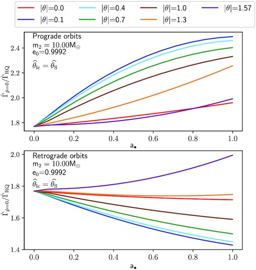
$Ratio $\dot{\Gamma }_{\dot{p}=0}/\dot{\Gamma }_{\rm RQ}$ as a function of the spin a• for a BH EMRI approaching a central MBH of mass MMBH = 4.3 × 106 M⊙. The colours represent the different orbital inclinations, θ, given in radians. The top (bottom) panel shows the prograde (retrograde) cases.$

Figure 6.

Ratio |$\dot{\Gamma }_{\dot{p}=0}/\dot{\Gamma }_{\rm RQ}$| as a function of the spin a_• for a BH EMRI approaching a central MBH of mass M_MBH = 4.3 × 10⁶ M_⊙. The colours represent the different orbital inclinations, θ, given in radians. The top (bottom) panel shows the prograde (retrograde) cases.

Open in new tab Download slide

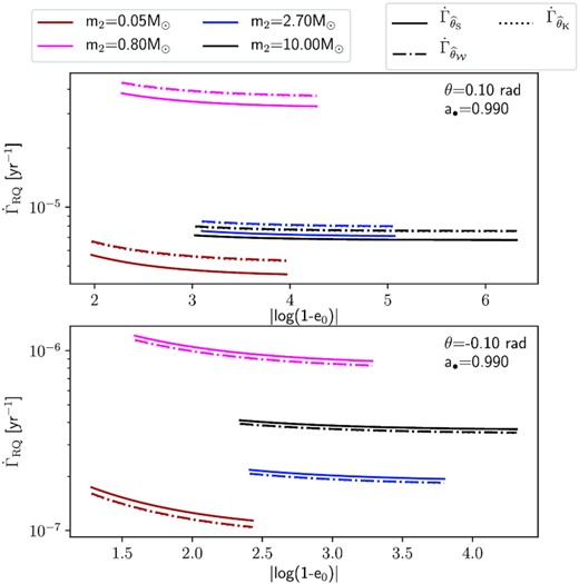
Finally, for the eccentricity range given in Table 3, we plot in Fig. 7 the rates |$\dot{\Gamma }_{\rm RQ}$| and |$\dot{\Gamma }_{\dot{p}=0}$| for objects with orbital inclinations θ = ±0.1 rad approaching a Kerr MBH of mass M_MBH = 4.3 × 10⁶ M_⊙ and a_• = 0.999. Prograde WD EMRIs have the highest event rates with |$\dot{\Gamma }_{\dot{p}=0}\sim 1.5\times 10^{-4}$| yr⁻¹ and |$\dot{\Gamma }_{\rm RQ}\sim 5\times 10^{-5}$| yr⁻¹. For NS EMRIs we obtain |$\dot{\Gamma }_{\dot{p}=0}\sim 3.2\times 10^{-5}$| yr⁻¹, and |$\dot{\Gamma }_{\dot{p}=0}\gtrsim 2\times 10^{-5}$| yr⁻¹ for BH EMRIs, and BD X-MRIs. The corrected version gives |$\dot{\Gamma }_{\rm RQ}\sim 1 \times 10^{-5}$| yr⁻¹ for NS EMRIs, |$\dot{\Gamma }_{\rm RQ}\gtrsim 9 \times 10^{-6}$| yr⁻¹ for BH EMRIs, and |$\dot{\Gamma }_{\rm RQ}\sim 6.5 - 8 \times 10^{-6}$| yr⁻¹ for BD X-MRIs.

$Inspiral event rates for prograde (upper panel) and retrograde orbits (lower panel) with |θ| = 0.1 rad, around a central MBH (MMBH = 4.3 × 106 M⊙) with a• = 0.999; $\dot{\Gamma }_{\dot{p}=0}$ (dotted lines) is obtained with the time-scale $T_{\dot{p}=0}$ (equation 3), whereas $\dot{\Gamma }_{\rm RQ}$ (solid lines) comes from equation (29). Brown lines represent a BD (m2 = 0.05 M⊙) X-MRI, blue lines an NS (m2 = 2.7 M⊙) EMRI, pink lines a WD (m2 = 0.8 M⊙) EMRI, and black lines a stellar-mass BH (m2 = 10 M⊙) EMRI.$

Figure 7.

Inspiral event rates for prograde (upper panel) and retrograde orbits (lower panel) with |θ| = 0.1 rad, around a central MBH (M_MBH = 4.3 × 10⁶ M_⊙) with a_• = 0.999; |$\dot{\Gamma }_{\dot{p}=0}$| (dotted lines) is obtained with the time-scale |$T_{\dot{p}=0}$| (equation 3), whereas |$\dot{\Gamma }_{\rm RQ}$| (solid lines) comes from equation (29). Brown lines represent a BD (m₂ = 0.05 M_⊙) X-MRI, blue lines an NS (m₂ = 2.7 M_⊙) EMRI, pink lines a WD (m₂ = 0.8 M_⊙) EMRI, and black lines a stellar-mass BH (m₂ = 10 M_⊙) EMRI.

Open in new tab Download slide

The highest event rate of the retrograde cases is also obtained for WD EMRIs with |$\dot{\Gamma }_{\dot{p}=0}\sim 1.4\times 10^{-6}$| yr⁻¹ and |$\dot{\Gamma }_{\rm RQ}\sim 1.2\times 10^{-6} - 8.6 \times 10^{-7}$| yr⁻¹. For retrograde BH EMRIs, NS EMRIs, and BD X-MRIs, the event rates are ∼10⁻⁷ yr⁻¹, and |$\dot{\Gamma }_{\rm RQ}\lesssim \dot{\Gamma }_{\dot{p}=0}$|⁠, with the only exception occurring at e₀ ≲ 0.95, where |$\dot{\Gamma }_{\dot{p}=0}\lesssim \dot{\Gamma }_{\rm RQ}$| for BD X-MRIs. These values remain approximately constant along the eccentricity range, the largest variation occurring for retrograde BD X-MRIs, where there is a difference of a factor ∼1.5 between the values of |$\dot{\Gamma }_{\rm RQ}$| evaluated at e_min and e_max.

Note that |$\dot{\Gamma }_{\rm RQ}$| gives an upper limit for the event rate when θ = 0.1 rad, because p₀ < 3r_S and the correction factor Q is evaluated at p₀ = 3r_S, whereas for θ = −0.1 rad |$\dot{\Gamma }_{\rm RQ}$| contains the full PN correction as p₀ > 3r_S.

LISA will be able to detect EMRIs and X-MRIs if the mass of the central MBH is between ∼10⁴ M_⊙ and ∼ 10⁷ M_⊙. For lower MBH masses, the GWs amplitude would be very low and the source would need to be located within a few Gpc to be detected (Gair et al. 2004; Amaro-Seoane et al. 2007). On the other hand, if the mass of the MBH is higher than ∼10⁷ M_⊙, the signal’s frequency would be too low to be detected.

Black holes at the low-mass end (∼10^4 − 5 M_⊙) can be identified as intermediate-mass black holes (IMBHs). Although their existence and the validity of the scaling relations remain uncertain, kinematic observations of globular clusters and dwarf galaxies seem to indicate the presence of IMBHs in the central region of these stellar systems (Lützgendorf et al. 2013, 2014; Tremou et al. 2018; Reines & Volonteri 2015; Baldassare et al. 2020).

The description presented in this work can be extended to systems with M_MBH ∈ [10⁴, 10⁷] M_⊙, assuming that scaling relations between the central MBH and the host’s stellar system holds for this MBH mass range. In that case, the critical semimajor axis scales as

$$\begin{eqnarray*} a_{\rm crit}& \sim & 5.33 \times 10^{-1}\, \text{pc} \, \times \mathcal {R}\, \mathcal {Z} \left(\mathcal {N}\, \hat{e}\right)^{-4/5}\times \nonumber \\ &&\times \, \left(\frac{m_{\rm BH}}{10\, \mathrm{M}_{\odot }}\right)^{-8/5} \left(\frac{10\, \mathrm{M}_{\odot }}{m_{2}}\right)^{-4/5} \left[ \frac{4.3\times 10^6 \, \mathrm{M}_{\odot }}{M_{\rm MBH}}\right]^{-4/5}, \nonumber\\ \end{eqnarray*}$$

(33)

where we take an eccentricity of 0.9992 so that

$$\begin{eqnarray*} \hat{e}\approx \left(\frac{1}{1.28}\right) \frac{f(e_0)}{\big(1-e_0^2\big)(1-e_0)^{5/2}}, \end{eqnarray*}$$

and

$$\begin{eqnarray*} \mathcal {R}&=& \left(\frac{R_{\rm h}}{1 \text{pc}}\right), \, \mathcal {N}=\frac{N_0}{12000} \frac{\text{ln}(\Lambda)}{13},\nonumber \\ \mathcal {Z}&=& (R\, Q)^{-4/5} \mathcal {W}(\theta , a_{\bullet })^{-2}. \end{eqnarray*}$$

(34)

The event rate for m₂ = m_BH = 10 M_⊙, β = γ = 7/4, and |$\widehat{\theta }_{\rm lc}=\widehat{\theta }_{\rm S}$|⁠, scales as

$$\begin{eqnarray*} \dot{\Gamma }_{\rm i} &\sim & 7.76\times 10^{-8}\, \text{yr}^{-1} \, \times \mathcal {R}^{-4/5} \mathcal {N}^{1/5} \left(\frac{M_{\rm MBH}}{4.3\times 10^6 \, \mathrm{M}_{\odot }}\right)^{3/5} \nonumber\\ &&\times \,\Bigg \lbrace \mathcal {Z} \, \hat{e}^{-4/5} \times \Bigg [ 96 + \text{ln} \left(\mathcal {Z} \, \mathcal {R} \left(\mathcal {N} \hat{e} \right)^{-4/5}\right. \nonumber\\ &&\left.\times \,\left(\frac{M_{\rm MBH}}{4.3\times 10^6 \, \mathrm{M}_{\odot }} \right)^{-1/5} \right) \Bigg ] \nonumber \\ &&-\, 9.6\times 10^{-6} \mathcal {N}^{-4/5} \left(\frac{M_{\rm MBH}}{4.3\times 10^6 \, \mathrm{M}_{\odot }}\right)^{8/5} \nonumber \\ &&\times \left[ 89+\text{ln}\left(\mathcal {R} \left(\frac{M_{\rm MBH}}{4.3\times 10^6 \, \mathrm{M}_{\odot }}\right)^{-8/5}\right)\right]\Bigg \rbrace . \end{eqnarray*}$$

(35)

Note that to obtain the correct value for a_crit and |$\dot{\Gamma }_{\rm i}$|⁠, the term |$\mathcal {Z}$| has to be evaluated. Neither the function |$\mathcal {W}(\theta , a_{\bullet })$| nor the correction factors RQ (equations 4, 17 and 18) depend on the mass of the MBH or m₂. Therefore, the effect of the term |$\mathcal {Z}$| in the last equation is fixed for a given set of a_•, θ, and e₀; it decreases the event rates by a factor that remains between ≲0.9 and ≳3 for the different orbital inclinations and spin value.

Fig. 8 shows |$\dot{\Gamma }_{\rm RQ}$|⁠, and |$\dot{\Gamma }_{\dot{p}=0}$|⁠, obtained for a BH EMRI with orbital inclinations θ = 1.57 rad and θ = 0.1 rad, around a central MBH of mass M_MBH ∈ [10⁴, 10⁷] M_⊙, a_• = [0, 0.999], and e₀ = e_min (equation 32). To compute the value of e₀, we assume that the M–σ relation for the velocity dispersion described in Tremaine et al. (2002), |$\sigma _0 \sim 200~(M_{\rm MBH}/10^8\, {\rm M}_{\odot })^{1/4}$| km s⁻¹, holds for the considered MBH masses. The event rate decreases with the mass of the central MBH; also, as the value of e_min depends on M_MBH and R_h, EMRIs in the low-mass end are more eccentric compared to EMRIs formed around the most massive central MBHs; a similar behaviour occurs if we take e₀ = e_max, since the magnitude of a_crit also decreases with the mass of the central MBH.

$Event rates $\dot{\Gamma }_{\rm RQ}$, and $\dot{\Gamma }_{\dot{p}=0}$, obtained with $\widehat{\theta }_{\rm S}$ and e0 = emin, for an EMRI composed of a BH of mass m2 = 10 M⊙ and a central MBH of mass MMBH ∈ [104, 107] M⊙. Black and coloured lines represent the Schwarzschild and Kerr case (a• = 0.999) case, respectively. Blue and purple lines are obtained for the orbital inclination θ = 0.1 rad and θ = 1.57 rad, respectively.$

Figure 8.

Event rates |$\dot{\Gamma }_{\rm RQ}$|⁠, and |$\dot{\Gamma }_{\dot{p}=0}$|⁠, obtained with |$\widehat{\theta }_{\rm S}$| and e₀ = e_min, for an EMRI composed of a BH of mass m₂ = 10 M_⊙ and a central MBH of mass M_MBH ∈ [10⁴, 10⁷] M_⊙. Black and coloured lines represent the Schwarzschild and Kerr case (a_• = 0.999) case, respectively. Blue and purple lines are obtained for the orbital inclination θ = 0.1 rad and θ = 1.57 rad, respectively.

Open in new tab Download slide

Fig. 9 shows the ratio |$\dot{\Gamma }_{\dot{p}=0}/\dot{\Gamma }_{\rm RQ}$| for the same EMRI configuration. As the effect of the spin is weak on highly inclined orbits (θ = 1.57 rad), the effect of the eccentricity becomes more important, increasing the ratio |$\dot{\Gamma }_{\dot{p}=0}/\dot{\Gamma }_{\rm RQ}$| as M_MBH → 10⁴ M_⊙. For M_MBH = 10⁷M_⊙, the eccentricity value is ∼0.995, so the effect of the RQ corrections is weaker than for the less massive MBHs where e₀ → 0.999999. On the other hand, for θ = 0.1 rad, the influence of the spin dominates over the eccentricity evolution and PN effects are stronger; |$\dot{\Gamma }_{\dot{p}=0}/\dot{\Gamma }_{\rm RQ}\sim 2.6$|–2.7 along the MBH’s mass range.

$Ratio $\dot{\Gamma }_{\dot{p}=0}/\dot{\Gamma }_{\rm RQ}$, for a BH EMRI with a central MBH with mass MMBH ∈ [104, 107] M⊙. Black and coloured lines represent the Schwarzschild and Kerr case (a• = 0.999) case, respectively. Blue and purple lines are obtained for the orbital inclination θ = 0.1 rad and θ = 1.57 rad, respectively. The event rates are obtained considering $\widehat{\theta }_{\rm S}$ and e0 = emin.$

Figure 9.

Ratio |$\dot{\Gamma }_{\dot{p}=0}/\dot{\Gamma }_{\rm RQ}$|⁠, for a BH EMRI with a central MBH with mass M_MBH ∈ [10⁴, 10⁷] M_⊙. Black and coloured lines represent the Schwarzschild and Kerr case (a_• = 0.999) case, respectively. Blue and purple lines are obtained for the orbital inclination θ = 0.1 rad and θ = 1.57 rad, respectively. The event rates are obtained considering |$\widehat{\theta }_{\rm S}$| and e₀ = e_min.

Open in new tab Download slide

5.2 The effect of the loss-cone angle

The shift in the LSO position can reduce or increase the magnitude of the loss-cone angle, modifying the phase-space volume that places the pericentre of an orbit inside the LSO. As a_• → 1, the Kerr loss-cone angles |$\widehat{\theta }_{\mathcal {W}}$| and |$\widehat{\theta }_{\rm K}$| (equations 26 and 28) deviate more from the Schwarzschild loss-cone angle |$\widehat{\theta }_{\rm S}$|⁠. However, the change in the event rates is small even for high spin values, as |$\dot{\Gamma }_{\rm i} \propto \ln (\widehat{\theta }^{-2}_{\rm lc})$|⁠.

The factor Q indicates that the influence of a_• and θ is not as large as the one obtained when the function |$\mathcal {W}(\theta ,a_{\bullet })$| is implemented (see Table 5), so it is no surprise that the rates |$\dot{\Gamma }_{\dot{p}=0}$| are more affected by |$\widehat{\theta }_{\mathcal {W}}$| and |$\widehat{\theta }_{\rm K}$| compared to |$\dot{\Gamma }_{\rm RQ}$|⁠.

By computing |$\dot{\Gamma }_{\rm RQ}$| and |$\dot{\Gamma }_{\dot{p}=0}$| with |$\widehat{\theta }_{\rm lc}=\widehat{\theta }_{\rm S}$|⁠, |$\widehat{\theta }_{\mathcal {W}}$|⁠, and |$\widehat{\theta }_{\rm K}$| for a spin value of a_• = 0.99 that guarantees the accuracy within 5 per cent of J_crit (equation 27), we find that the asymmetric effect of the MBH spin is still noticeable. It can be seen in Fig. 10, where we show the corrected event rates computed with the different loss-cone angles – |$\dot{\Gamma }_{\widehat{\theta }_{\rm S}}$|⁠, |$\dot{\Gamma }_{\widehat{\theta }_{\mathcal {W}}}$|⁠, and |$\dot{\Gamma }_{\widehat{\theta }_{\rm K}}$| – as a function of e₀ for the considered EMRIs and X-MRIs.

$Event rates $\dot{\Gamma }_{\rm RQ}$ computed with the different loss-cone angles, as a function of e0 for EMRIs and X-MRIs with |θ| = 0.1 rad in prograde (upper panel), and retrograde orbits (lower panel), around a MBH of mass MMBH = 4.3 × 106 M⊙, and a• = 0.99. The subscript indicates which loss-cone angle is used to obtain the event rates; $\widehat{\theta }_{\rm S}$ is given by equation (25), $\widehat{\theta }_{\mathcal {W}}$ is the Kerr loss-cone angle given by equation (26), and $\widehat{\theta }_{\rm K}$ is given by equation (28).$

Figure 10.

Event rates |$\dot{\Gamma }_{\rm RQ}$| computed with the different loss-cone angles, as a function of e₀ for EMRIs and X-MRIs with |θ| = 0.1 rad in prograde (upper panel), and retrograde orbits (lower panel), around a MBH of mass M_MBH = 4.3 × 10⁶ M_⊙, and a_• = 0.99. The subscript indicates which loss-cone angle is used to obtain the event rates; |$\widehat{\theta }_{\rm S}$| is given by equation (25), |$\widehat{\theta }_{\mathcal {W}}$| is the Kerr loss-cone angle given by equation (26), and |$\widehat{\theta }_{\rm K}$| is given by equation (28).

Open in new tab Download slide

In Section 4.2, we showed that, for prograde orbits around a Kerr MBH, |$\widehat{\theta }_{\mathcal {W}}\sim \widehat{\theta }_{\rm K}$|⁠, and that, for high spin values, |$\widehat{\theta }_{\mathcal {W}}\lesssim$| 0.5 |$\widehat{\theta }_{\rm S}$|⁠. This reduction in the loss-cone angle increases the EMRI and X-MRI event rates |$\dot{\Gamma }_{\dot{p}=0}$| by a factor ∼1.2 compared to the Schwarzschild case. For objects in retrograde orbits, |$\dot{\Gamma }_{\dot{p}=0}$| are reduced by a factor ∼0.8 due to the small increase in the magnitude of the Kerr loss-cone angle. In the case of |$\dot{\Gamma }_{\rm RQ}$|⁠, the Kerr loss-cone angle changes the rates estimate by a factor ∼0.9 to ∼1.1, which is still negligible. In Table 6, we give the ratio between these rates.

Table 6.

Open in new tab

Comparison of event rates computed with |$\widehat{\theta }_{\rm S}$| and the Kerr loss-cone angles |$\widehat{\theta }_{\mathcal {W}}$| and |$\widehat{\theta }_{\rm K}$| for each inspiraling object. We take θ = ±0.1 rad, M_MBH = 4.3 × 10⁶ M_⊙, and a_• = 0.99. The upper section shows the change induced by the Kerr loss-cone angles in |$\dot{\Gamma }_{\rm RQ}$| and the lower part shows the change in |$\dot{\Gamma }_{\dot{p}=0}$|⁠.

\|$\dot{\Gamma }_{\rm RQ}$\|	\|$\dot{\Gamma }_{\widehat{\theta }_{\mathcal {W}}}/\dot{\Gamma }_{\widehat{\theta }_{\rm S}}$\|		\|$\dot{\Gamma }_{\widehat{\theta }_{\rm K}}/\dot{\Gamma }_{\widehat{\theta }_{\rm S}}$\|
θ [rad]	0.1	−0.1	0.1	−0.1
BD	1.17	0.92	1.16	0.92
WD	1.13	0.94	1.12	0.94
NS	1.12	0.95	1.11	0.95
BH	1.11	0.95	1.10	0.95
\|$\dot{\Gamma }_{\dot{p}=0}$\|	\|$\dot{\Gamma }_{\widehat{\theta }_{\mathcal {W}}}/\dot{\Gamma }_{\widehat{\theta }_{\rm S}}$\|		\|$\dot{\Gamma }_{\widehat{\theta }_{\rm K}}/\dot{\Gamma }_{\widehat{\theta }_{\rm S}}$\|
θ [rad]	0.1	−0.1	0.1	−0.1
BD	1.22	0.89	1.21	0.88
WD	1.16	0.93	1.15	0.92
NS	1.14	0.94	1.13	0.93
BH	1.13	0.94	1.12	0.94

\|$\dot{\Gamma }_{\rm RQ}$\|	\|$\dot{\Gamma }_{\widehat{\theta }_{\mathcal {W}}}/\dot{\Gamma }_{\widehat{\theta }_{\rm S}}$\|		\|$\dot{\Gamma }_{\widehat{\theta }_{\rm K}}/\dot{\Gamma }_{\widehat{\theta }_{\rm S}}$\|
θ [rad]	0.1	−0.1	0.1	−0.1
BD	1.17	0.92	1.16	0.92
WD	1.13	0.94	1.12	0.94
NS	1.12	0.95	1.11	0.95
BH	1.11	0.95	1.10	0.95
\|$\dot{\Gamma }_{\dot{p}=0}$\|	\|$\dot{\Gamma }_{\widehat{\theta }_{\mathcal {W}}}/\dot{\Gamma }_{\widehat{\theta }_{\rm S}}$\|		\|$\dot{\Gamma }_{\widehat{\theta }_{\rm K}}/\dot{\Gamma }_{\widehat{\theta }_{\rm S}}$\|
θ [rad]	0.1	−0.1	0.1	−0.1
BD	1.22	0.89	1.21	0.88
WD	1.16	0.93	1.15	0.92
NS	1.14	0.94	1.13	0.93
BH	1.13	0.94	1.12	0.94

Table 6.

Open in new tab

Comparison of event rates computed with |$\widehat{\theta }_{\rm S}$| and the Kerr loss-cone angles |$\widehat{\theta }_{\mathcal {W}}$| and |$\widehat{\theta }_{\rm K}$| for each inspiraling object. We take θ = ±0.1 rad, M_MBH = 4.3 × 10⁶ M_⊙, and a_• = 0.99. The upper section shows the change induced by the Kerr loss-cone angles in |$\dot{\Gamma }_{\rm RQ}$| and the lower part shows the change in |$\dot{\Gamma }_{\dot{p}=0}$|⁠.

\|$\dot{\Gamma }_{\rm RQ}$\|	\|$\dot{\Gamma }_{\widehat{\theta }_{\mathcal {W}}}/\dot{\Gamma }_{\widehat{\theta }_{\rm S}}$\|		\|$\dot{\Gamma }_{\widehat{\theta }_{\rm K}}/\dot{\Gamma }_{\widehat{\theta }_{\rm S}}$\|
θ [rad]	0.1	−0.1	0.1	−0.1
BD	1.17	0.92	1.16	0.92
WD	1.13	0.94	1.12	0.94
NS	1.12	0.95	1.11	0.95
BH	1.11	0.95	1.10	0.95
\|$\dot{\Gamma }_{\dot{p}=0}$\|	\|$\dot{\Gamma }_{\widehat{\theta }_{\mathcal {W}}}/\dot{\Gamma }_{\widehat{\theta }_{\rm S}}$\|		\|$\dot{\Gamma }_{\widehat{\theta }_{\rm K}}/\dot{\Gamma }_{\widehat{\theta }_{\rm S}}$\|
θ [rad]	0.1	−0.1	0.1	−0.1
BD	1.22	0.89	1.21	0.88
WD	1.16	0.93	1.15	0.92
NS	1.14	0.94	1.13	0.93
BH	1.13	0.94	1.12	0.94

\|$\dot{\Gamma }_{\rm RQ}$\|	\|$\dot{\Gamma }_{\widehat{\theta }_{\mathcal {W}}}/\dot{\Gamma }_{\widehat{\theta }_{\rm S}}$\|		\|$\dot{\Gamma }_{\widehat{\theta }_{\rm K}}/\dot{\Gamma }_{\widehat{\theta }_{\rm S}}$\|
θ [rad]	0.1	−0.1	0.1	−0.1
BD	1.17	0.92	1.16	0.92
WD	1.13	0.94	1.12	0.94
NS	1.12	0.95	1.11	0.95
BH	1.11	0.95	1.10	0.95
\|$\dot{\Gamma }_{\dot{p}=0}$\|	\|$\dot{\Gamma }_{\widehat{\theta }_{\mathcal {W}}}/\dot{\Gamma }_{\widehat{\theta }_{\rm S}}$\|		\|$\dot{\Gamma }_{\widehat{\theta }_{\rm K}}/\dot{\Gamma }_{\widehat{\theta }_{\rm S}}$\|
θ [rad]	0.1	−0.1	0.1	−0.1
BD	1.22	0.89	1.21	0.88
WD	1.16	0.93	1.15	0.92
NS	1.14	0.94	1.13	0.93
BH	1.13	0.94	1.12	0.94

6 DISCUSSION AND CONCLUSIONS

The spin of the MBH and the orbital inclination of the inspiraling object can not be ignored; these quantities can affect the event rates in two forms. Firstly, through the pericentre of an inspiraling orbit: as we fix the pericentre at r_LSO, a shift in the LSO position changes the value of the critical semimajor axis and the integration volume of equation (20), significantly enhancing the event rates of prograde orbits, and slightly reducing the event rates in the retrograde cases, as the effect of the MBH spin is not symmetric. Secondly, through the loss-cone: its value also depends on r_LSO and determines the set of velocity vectors that take an object to a direct plunge. We give two expressions, |$\widehat{\theta }_{\mathcal {W}}$| and |$\widehat{\theta }_{\rm K}$|⁠, to obtain a loss-cone angle that accounts for spin effects. Both versions of the Kerr loss-cone angle give similar results and, as a_• → 1, |$\widehat{\theta }_{\mathcal {W}}$| and |$\widehat{\theta }_{\rm K}$| deviate more from the Schwarzschild case |$\widehat{\theta }_{\rm S}$|⁠. However, we find that the influence of the MBH spin added through the pericentre condition, p₀ = r_LSO, already contains the most relevant effects regarding the event rates, so that implementing |$\widehat{\theta }_{\mathcal {W}}$| or |$\widehat{\theta }_{\rm K}$| changes the event rates by a factor that ranges between 0.9 and 1.2, which does not produce a significant impact on the rate estimates.

We obtained event rates for EMRIs and X-MRIs by implementing three different merger time-scales, T_P, T_RQ, and |$T_{\dot{p}=0}$|⁠. Peters’ formula, T_P, overestimates the energy loss by GWs and fails to give an accurate merger time-scale; this can be avoided by including eccentricity evolution and post-Newtonian corrections through the correction factors R and Q; the resulting time-scale, T_RQ, is longer than T_P and produces the best merger time-scale estimate for arbitrary eccentricities, orbital inclinations, and MBH spin values. The alternative formulation |$T_{\dot{p}=0}$| gives a reliable estimate of the merger time-scale, |$T_{\dot{p}=0} \lesssim T_{\rm RQ}$|⁠, in the context of EMRIs and X-MRIs. However, for arbitrary values of e₀, θ, or a_•, its accuracy can not be guaranteed.

We have shown that for the eccentricity range and pericentre distances expected for EMRIs and X-MRIs (e₀ > 0.9, p₀ = r_LSO), implementing T_GW = T_P results in unreliable event rates estimates. |$\dot{\Gamma }_{\rm P}$| are artificially enhanced by a factor that ranges between ∼8 to 30 compared to the corrected values |$\dot{\Gamma }_{\rm RQ}$|⁠. On the other hand, the estimates given by |$\dot{\Gamma }_{\dot{p}=0}$|⁠, which include the influence of the MBH spin and the orbital inclination through the function |$\mathcal {W}(\theta , a_{\bullet })$|⁠, differ from |$\dot{\Gamma }_{\rm RQ}$| by a factor between 0.9 and 3.

We conclude that both the Kerr loss-cone and the RQ corrections to Peters’ time-scale do not have a dramatic impact on the event rates for EMRIs or X-MRIs, when compared to the high-eccentricity approach of Amaro-Seoane et al. (2013). However, this work considers only the dynamical and relativistic aspects of the EMRIs and X-MRIs formation and considers the galactic nucleus of the Milky Way as a representative example of the galaxies that could harbour potential inspiral sources. If EMRIs and X-MRIs in Nature happened to form at very low eccentricities, or if environmental effects (not included in this work; e.g. torques induced by background gas) can induce a significant reduction of the initial eccentricity of EMRIs and X-MRIs (e₀ ≲ 0.8), it would be necessary to implement the eccentricity-evolution and PN corrections to obtain accurate event rate estimates. In any case, all event rates for MBH binaries and stellar-mass binaries should be revisited using our improvements because their eccentricities will span through all possible values. Furthermore, our description holds for MBHs with masses between ∼10⁴ M_⊙ and ∼10⁷ M_⊙, covering the mass interval detectable by LISA.

ACKNOWLEDGEMENTS

VVA acknowledges support from CAS-TWAS President’s PhD Fellowship Programme of the Chinese Academy of Sciences & The World Academy of Sciences. PAS acknowledges support from the Ramón y Cajal Programme of the Ministry of Economy, Industry and Competitiveness of Spain, as well as the financial support of Programa Estatal de Generación de Conocimiento (ref. PGC2018-096663-B-C43) (MCIU/FEDER). This work was supported by the National Key R&D Program of China (2016YFA0400702) and the National Science Foundation of China (11721303, 11873022 and 11991053). PRC, LM, and LZ acknowledge support from the Swiss National Science Foundation under the Grant 200020_178949. EB acknowledges support from the European Research Council (ERC) under the European Union’s Horizon 2020 research and innovation program ERC-2018-COG under grant agreement N. 818691 (B Massive).

DATA AVAILABILITY STATEMENT

The data underlying this article will be shared on reasonable request to the corresponding author.

Footnotes

1

We define the MBH spin as |$a_\bullet = c J_{\rm MBH} /(G M_{\rm MBH}^2)$|⁠, where M_MBH and J_MBH are the MBH’s mass and angular momentum magnitude, respectively, c is the speed of light in vacuum, and G is the gravitational constant.

REFERENCES

Alexander

T.

,

Hopman

C.

,

2003

,

ApJ

,

590

,

L29

10.1086/376672

Crossref

Search ADS

Alexander

T.

,

Hopman

C.

,

2009

,

ApJ

,

697

,

1861

10.1088/0004-637X/697/2/1861

Crossref

Search ADS

Amaro-Seoane

P.

,

2018

,

Living Rev. Relativ.

,

21

,

4

10.1007/s41114-018-0013-8

Crossref

Search ADS

PubMed

Amaro-Seoane

P.

,

2019

,

Phys. Rev. D

,

99

,

123025

10.1103/PhysRevD.99.123025

Crossref

Search ADS

Amaro-Seoane

P.

,

2020

,

preprint (arXiv:2011.03059)

Amaro-Seoane

P.

,

Preto

M.

,

2011

,

Classical and Quantum Gravity

,

28

,

094017

10.1088/0264-9381/28/9/094017

Crossref

Search ADS

Amaro-Seoane

P.

,

Freitag

M.

,

Spurzem

R.

,

2004

,

MNRAS

,

352

,

655

10.1111/j.1365-2966.2004.07956.x

Crossref

Search ADS

Amaro-Seoane

P.

,

Gair

J. R.

,

Freitag

M.

,

Miller

M. C.

,

Mandel

I.

,

Cutler

C. J.

,

Babak

S.

,

2007

,

Classical and Quantum Gravity

,

24

,

113

10.1088/0264-9381/24/17/R01

Crossref

Search ADS

Amaro-Seoane

P.

et al. ,

2012

,

Classical and Quantum Gravity

,

29

,

124016

10.1088/0264-9381/29/12/124016

Crossref

Search ADS

Amaro-Seoane

P.

,

Sopuerta

C. F.

,

Freitag

M. D.

,

2013

,

MNRAS

,

429

,

3155

10.1093/mnras/sts572

Crossref

Search ADS

Babak

S.

et al. ,

2017

,

Phys. Rev. D

,

95

,

103012

10.1103/PhysRevD.95.103012

Crossref

Search ADS

Bahcall

J. N.

,

Wolf

R. A.

,

1976

,

ApJ

,

209

,

214

10.1086/154711

Crossref

Search ADS

Baldassare

V. F.

,

Dickey

C.

,

Geha

M.

,

Reines

A. E.

,

2020

,

ApJ

,

898

,

L3

10.3847/2041-8213/aba0c1

Crossref

Search ADS

Barack

L.

,

Cutler

C.

,

2004

,

Phys. Rev. D

,

69

,

082005

10.1103/PhysRevD.69.082005

Crossref

Search ADS

Barack

L.

et al. ,

2019

,

Classical and Quantum Gravity

,

36

,

143001

10.1088/1361-6382/ab0587

Crossref

Search ADS

Baumgardt

H.

,

Makino

J.

,

Ebisuzaki

T.

,

2004a

,

ApJ

,

613

,

1133

10.1086/423298

Crossref

Search ADS

Baumgardt

H.

,

Makino

J.

,

Ebisuzaki

T.

,

2004b

,

ApJ

,

613

,

1143

10.1086/423299

Crossref

Search ADS

Baumgardt

H.

,

Amaro-Seoane

P.

,

Schödel

R.

,

2018

,

A&A

,

609

,

A28

10.1051/0004-6361/201730462

Crossref

Search ADS

Binney

J.

,

Tremaine

S.

,

1987

,

Galactic dynamics

.

Princeton Univ. Press

,

Princeton

Google Scholar

Google Preview

OpenURL Placeholder Text

WorldCat

Bonetti

M.

,

Perego

A.

,

Capelo

P. R.

,

Dotti

M.

,

Miller

M. C.

,

2018

,

PASA

,

35

,

e017

10.1017/pasa.2018.11

Crossref

Search ADS

Brown

W. R.

,

Geller

M. J.

,

Kenyon

S. J.

,

Kurtz

M. J.

,

2005

,

ApJ

,

622

,

L33

10.1086/429378

Crossref

Search ADS

Einstein

A.

,

1916

,

Annalen der Physik

,

354

,

769

10.1002/andp.19163540702

Crossref

Search ADS

Freitag

M.

,

Benz

W.

,

2001

,

A&A

,

375

,

711

10.1051/0004-6361:20010706

Crossref

Search ADS

Freitag

M.

,

Benz

W.

,

2002

,

A&A

,

394

,

345

10.1051/0004-6361:20021142

Crossref

Search ADS

Freitag

M.

,

Amaro-Seoane

P.

,

Kalogera

V.

,

2006

,

Journal of Physics Conference Series

,

54

,

252

Google Scholar

Google Preview

OpenURL Placeholder Text

WorldCat

Gair

J. R.

,

Barack

L.

,

Creighton

T.

,

Cutler

C.

,

Larson

S. L.

,

Phinney

E. S.

,

Vallisneri

M.

,

2004

,

Classical and Quantum Gravity

,

21

,

S1595

10.1088/0264-9381/21/20/003

Crossref

Search ADS

Gair

J. R.

,

Kennefick

D. J.

,

Larson

S. L.

,

2006

,

ApJ

,

639

,

999

10.1086/499425

Crossref

Search ADS

Gallego-Cano

E.

,

Schödel

R.

,

Dong

H.

,

Nogueras-Lara

F.

,

Gallego-Calvente

A. T.

,

Amaro-Seoane

P.

,

Baumgardt

H.

,

2018

,

A&A

,

609

,

A26

10.1051/0004-6361/201730451

Crossref

Search ADS

Hills

J. G.

,

1988

,

Nature

,

331

,

687

10.1038/331687a0

Crossref

Search ADS

Hopman

C.

,

Alexander

T.

,

2005

,

ApJ

,

629

,

362

10.1086/431475

Crossref

Search ADS

Kerr

R. P.

,

1963

,

Phys. Rev. Lett.

,

11

,

237

10.1103/PhysRevLett.11.237

Crossref

Search ADS

Klein

A.

et al. ,

2016

,

Phys. Rev. D

,

93

,

024003

10.1103/PhysRevD.93.024003

Crossref

Search ADS

Kroupa

P.

,

2001

,

MNRAS

,

322

,

231

10.1046/j.1365-8711.2001.04022.x

Crossref

Search ADS

Lützgendorf

N.

et al. ,

2013

,

A&A

,

555

,

A26

10.1051/0004-6361/201321183

Crossref

Search ADS

Lützgendorf

N.

et al. ,

2014

,

Proc. Int. Astron. Union

,

10

,

181

10.1017/s1743921315007784

Crossref

Search ADS

Merritt

D.

,

2013

,

Classical and Quantum Gravity

,

30

,

244005

10.1088/0264-9381/30/24/244005

Crossref

Search ADS

Peebles

P. J. E.

,

1972

,

ApJ

,

178

,

371

10.1086/151797

Crossref

Search ADS

Peters

P. C.

,

1964

,

PhD thesis

,

California Institute of Technology

Peters

P. C.

,

Mathews

J.

,

1963

,

Phys. Rev.

,

131

,

435

10.1103/PhysRev.131.435

Crossref

Search ADS

Preto

M.

,

Amaro-Seoane

P.

,

2009

,

ApJ

,

708

,

L42

10.1088/2041-8205/708/1/l42

Crossref

Search ADS

Reines

A. E.

,

Volonteri

M.

,

2015

,

ApJ

,

813

,

82

10.1088/0004-637x/813/2/82

Crossref

Search ADS

Schödel

R.

,

Gallego-Cano

E.

,

Dong

H.

,

Nogueras-Lara

F.

,

Gallego-Calvente

A. T.

,

Amaro-Seoane

P.

,

Baumgardt

H.

,

2018

,

A&A

,

609

,

A27

10.1051/0004-6361/201730452

Crossref

Search ADS

Schwarzschild

K.

,

1916

,

Abh. Konigl. Preuss. Akad. Wissenschaften Jahre 1906, 92, Berlin, 1907

,

1916

,

189

Sigurdsson

S.

,

Rees

M. J.

,

1997

,

MNRAS

,

284

,

318

10.1093/mnras/284.2.318

Crossref

Search ADS

Sopuerta

C. F.

,

Yunes

N.

,

2011

,

Phys. Rev. D

,

84

,

124060

10.1103/physrevd.84.124060

Crossref

Search ADS

Teukolsky

S.

,

Shapiro

S.

,

1983

,

Black holes, white dwarfs, and neutron stars: the physics of compact objects

.

Wiley

,

New York

Google Scholar

Google Preview

OpenURL Placeholder Text

WorldCat

Tremaine

S.

et al. ,

2002

,

apj

,

574

,

740

10.1086/341002

Crossref

Search ADS

Tremou

E.

et al. ,

2018

,

ApJ

,

862

,

16

10.3847/1538-4357/aac9b9

Crossref

Search ADS

Will

C. M.

,

2012

,

Classical and Quantum Gravity

,

29

,

217001

10.1088/0264-9381/29/21/217001

Crossref

Search ADS

Zwick

L.

,

Capelo

P. R.

,

Bortolas

E.

,

Mayer

L.

,

Amaro-Seoane

P.

,

2020

,

MNRAS

,

495

,

2321

10.1093/mnras/staa1314

Crossref

Search ADS

Zwick

L.

,

Capelo

P. R.

,

Bortolas

E.

,

Vázquez-Aceves

V.

,

Mayer

L.

,

Amaro-Seoane

P.

,

2021

,

MNRAS

,

506

,

1007

10.1093/mnras/stab1818

Crossref

Search ADS

This article is published and distributed under the terms of the Oxford University Press, Standard Journals Publication Model (https://dbpia.nl.go.kr/journals/pages/open_access/funder_policies/chorus/standard_publication_model)

Download all slides

Month:	Total Views:
December 2021	2
January 2022	33
February 2022	8
March 2022	10
April 2022	13
June 2022	8
July 2022	8
August 2022	3
September 2022	2
October 2022	4
November 2022	13
December 2022	3
January 2023	3
February 2023	2
March 2023	4
April 2023	4
May 2023	2
June 2023	2
August 2023	1
September 2023	9
October 2023	1
November 2023	5
December 2023	1
January 2024	32
February 2024	22
March 2024	8
April 2024	20
May 2024	18
June 2024	10
July 2024	15
August 2024	11
September 2024	24
October 2024	17
November 2024	17
December 2024	7
January 2025	10
February 2025	9
March 2025	25
April 2025	4
May 2025	11

Article Contents

Revised event rates for extreme and extremely large mass-ratio inspirals

ABSTRACT

1 INTRODUCTION

2 THE INSPIRAL TIME-SCALE

3 THE CRITICAL SEMIMAJOR AXIS

4 THE INSPIRAL EVENT RATE

4.1 Number of sources around an MBH

4.2 The loss-cone angle for Schwarzschild and Kerr black holes

5 EFFECT OF THE CORRECTION FACTORS AND THE LOSS-CONE ANGLE IN THE EVENT RATES

5.1 The effect of the correction factors

5.2 The effect of the loss-cone angle

6 DISCUSSION AND CONCLUSIONS

ACKNOWLEDGEMENTS

DATA AVAILABILITY STATEMENT

Footnotes

REFERENCES

Citations

Views

Altmetric

Email alerts

Astrophysics Data System

Citing articles via

Latest

Most Read

Most Cited

Article Contents

Revised event rates for extreme and extremely large mass-ratio inspirals

ABSTRACT

1 INTRODUCTION

2 THE INSPIRAL TIME-SCALE

3 THE CRITICAL SEMIMAJOR AXIS

4 THE INSPIRAL EVENT RATE

4.1 Number of sources around an MBH

4.2 The loss-cone angle for Schwarzschild and Kerr black holes

5 EFFECT OF THE CORRECTION FACTORS AND THE LOSS-CONE ANGLE IN THE EVENT RATES

5.1 The effect of the correction factors

5.2 The effect of the loss-cone angle

6 DISCUSSION AND CONCLUSIONS

ACKNOWLEDGEMENTS

DATA AVAILABILITY STATEMENT

Footnotes

REFERENCES

Citations

Views

Altmetric

Email alerts

Astrophysics Data System

Citing articles via

Latest

Most Read

Most Cited

This Feature Is Available To Subscribers Only