Observable gravitational waves from tidal disruption events and their electromagnetic counterpart

Pfister, Hugo; Toscani, Martina; Wong, Thomas Hong Tsun; Dai, Jane Lixin; Lodato, Giuseppe; Rossi, Elena M

doi:10.1093/mnras/stab3387

ABSTRACT

We estimate the rate of tidal disruption events (TDEs) that will be detectable with future gravitational wave detectors as well as the most probable properties of these events and their possible electromagnetic counterpart. To this purpose, we combine standard gravitational waves and electromagnetic results with detailed rates estimates. We find that the Laser Interferometer Space Antenna (LISA) should not detect any TDEs, unless black holes (BHs) are typically embedded by a young stellar population, which, in this situation, could lead up to few 10 events during the duration of the mission. If there are gravitational wave observations, these events should also be observable in the X-ray or the optical/UV part of the electromagnetic spectrum, which may open up the multimessenger era for TDEs. The generation of detectors following LISA will at least yearly observe 10⁴ TDEs at cosmological distances, allowing to do population studies and constrain the black hole mass function. In all cases, most probable events should be around black holes with a mass such that the Keplerian frequency at the Schwarzschild radius is similar to the optimal frequency of the detector and with a large penetration factor.

transients: tidal disruption events, gravitational waves

1 INTRODUCTION

If a star gets too close to a black hole (BH), the tidal force of the latter can disrupt the former. The stellar debris is then accreted by the BH, and this results in bright flares. These events are known as tidal disruption events (TDEs, Hills 1975; Lacy, Townes & Hollenbach 1982; Rees 1988), and they are now routinely detected by optical wide field surveys (e.g. van Velzen et al. 2020a; Jones et al. 2020).

The dynamics of the debris while falling on to the BH is a complex, non-linear problem that depends on orbital properties of the initial BH-star system (e.g. eccentricity and pericentre of the star, see Law-Smith et al. 2020; Ryu et al. 2020d), on the intrinsic properties of the star (e.g. internal structure: Lodato, King & Pringle 2009; Guillochon & Ramirez-Ruiz 2013; Goicovic et al. 2019; Golightly, Nixon & Coughlin 2019b; or rotation: Golightly, Coughlin & Nixon 2019a; Sacchi & Lodato 2019), and on the intrinsic properties of the BH (e.g. spin; Kesden 2012). None the less, several recent hydrodynamic codes allow to perform simulations of this problem (see review of Lodato et al. 2020), sometimes in a fully general relativistic context (Liptai et al. 2019; Ryu et al. 2020b, c). Since the evolution of the rate at which debris are accreted by the BH can be directly measured in these simulations, the time evolution of the luminosity can be directly mapped to the initial parameters of the TDE, and this idea has been recently exploited to reverse-engineer parameters of observed TDE light curves (Mockler, Guillochon & Ramirez-Ruiz 2019; Ryu, Krolik & Piran 2020a).

These extreme events involving massive BHs also result in the emission of gravitational waves, which also carry information about the nature of the system (Kobayashi et al. 2004; Stone et al. 2020; Toscani, Rossi & Lodato 2020). Gravitational waves being independent from electromagnetic waves, observing events in both domains allows us to better understand them: this is a branch of multimessenger astronomy, which has recently started with the spectacular observation of a binary neutron star merger both in the electromagnetic and the gravitational spectrum (Abbott et al. 2017). The future space-based gravitational wave detectors Laser Interferometer Space Antenna (LISA, Amaro-Seoane et al. 2017), TianQin (Luo et al. 2016), DECI-hertz inteferometer Gravitational wave Observatory (Decigo, Sato et al. 2009), Advanced Laser Interferometer Antenna (ALIA, Baker et al. 2019), and Big bang observatory (Bbo Harry et al. 2006) will be designed to study supermassive BHs. As such, one can naturally wonder if we will enter in the multimessenger astronomy era for TDEs, and what this will unveil about our understanding of BHs.

To address these questions, we estimate in this paper the expected rates that will be observed with these future gravitational wave detectors, what the properties of observed events will be, and if there will be any associated electromagnetic counterpart. We start by describing the conditions to observe a single event in Section 2; we then compute the rates for a global population of galaxies in Section 3; we finally give our results and conclusions in Section 4 and Section 5.

2 DETECTION OF SINGLE EVENTS

In this section, we assume that a TDE occurs at a given redshift (z): a star of mass and radius m_⋆ and r_⋆ plunges into a BH with mass M_•. The nearly parabolic orbit of the star is such that, at pericentre (r_p), it gets closer to the BH than the tidal radius (r_T = r_⋆(M_•/m_⋆)^1/3) where tidal force overcomes the stellar self-gravity, resulting in a TDE (we do not consider partial TDEs in this study and assume that stars are fully disrupted for r_p ≤ r_T, see Ryu et al. 2020c). During its journey, the star-BH system emits gravitational waves that may be detected when they arrive on Earth. In Section 2.1, we describe the formalism to define if a TDE is observable through gravitational waves and derive the maximum redshift for such observations; in Section 2.2, we perform the same exercise for the electromagnetic counterpart with the goal of determining whether multimessenger detectable events are likely or not.

2.1 Gravitational waves

2.1.1 Formalism

When a star orbiting a BH arrives at pericentre, the time-dependent mass quadrupole moment tensor of the system star-BH results in a burst of gravitational waves whose characteristic strain and frequency can be estimated as (Kobayashi et al. 2004; Stone et al. 2019):

$$\begin{eqnarray} h_\mathrm{GW} &=& \frac{2\, \mathrm{G}^2 m_\star M_\bullet }{\chi (z) c^4 r_\mathrm{ p}} \\ &=&10^{-22} \beta \left(\frac{\chi (z)}{16 \, \mathrm{Mpc}} \right)^{-1} \left(\frac{r_\star }{\, \mathrm{R}_{\odot }}\right)^{-1} \\ &&\times \left(\frac{m_\star }{\, \mathrm{M}_{\odot }}\right)^{4/3} \left(\frac{M_\bullet }{10^6\, \mathrm{M}_{\odot }}\right)^{2/3} \end{eqnarray}$$

(1)

$$\begin{eqnarray} f_\mathrm{GW} &=& \left(\frac{\, \mathrm{G}M_\bullet }{4\pi ^2 r_\mathrm{ p}^3}\right)^{1/2}\\ &=& 10^{-4} \, \mathrm{Hz}\times \beta ^{3/2} \left(\frac{m_\star }{\, \mathrm{M}_{\odot }}\right)^{1/2} \left(\frac{r_\star }{\, \mathrm{R}_{\odot }}\right)^{-3/2} \, , \end{eqnarray}$$

(2)

where χ(z) is the comoving distance (we assume a ΛCDM cosmology with Planck parameters; Planck Collaboration XIII 2016); β = r_T/r_p is the penetration factor (recall that in this study we have β ≥ 1 as we consider only full disruption of stars below the tidal radius); c and G are the speed of light and gravitational constant, respectively; and keeping in mind that the frequency is redshifted while travelling to Earth so that the observed frequency is:

$$\begin{eqnarray} f_\mathrm{obs} = \frac{f_\mathrm{GW}}{1+z} \, . \end{eqnarray}$$

(3)

For highly penetrating orbits, the star is swallowed whole resulting in a direct plunge. While this may result in the emission of observable gravitational waves, the debris would not form a luminous accretion disc, and there would not be any electromagnetic counterpart. In the simple ‘Newtonian picture with a BH of size the Schwarzschild radius of the BH’ |${r_\mathrm{Sch}=2\, \mathrm{G}M_\bullet /c^2}$|⁠, a star on parabolic orbit will directly plunge for r_p ≤ r_Sch. In the more realistic relativistic picture, the orbit of the star will follow the geodesic, and it is not straightforward to know what should be the initial pericentre of the parabolic orbit such that the star penetrates the BH. For simplicity, we only keep orbits with:

$$\begin{eqnarray} \beta \le \beta _\mathrm{max}&=& \frac{r_\mathrm{ T}}{\kappa r_\mathrm{Sch}} \end{eqnarray}$$

(4)

$$\begin{eqnarray} &=&\frac{r_\star c^2}{2 \kappa Gm_\star ^{1/3}M_\bullet ^{2/3}}\\ &=& 12 \left(\frac{\kappa }{2}\right)^{-1} \left(\frac{m_\star }{\, \mathrm{M}_{\odot }}\right)^{-1/3} \left(\frac{r_\star }{\, \mathrm{R}_{\odot }}\right) \left(\frac{M_\bullet }{10^6\, \mathrm{M}_{\odot }}\right)^{-2/3} , \end{eqnarray}$$

(5)

where κ indicates some critical radius (in units of r_Sch) for direct plunge. When it comes to the number of events per year, a larger κ naturally results in less TDEs, and vice versa. We tried with κ = 1 and κ = 2 and found the results to be changed by a factor of ∼2 only. However, since Kesden (2012) has shown that κ ∼ 2 nearly reproduced the correct relativistic rates (see their § IV.A.), we will use κ = 2 (r_p ≤ 2r_Sch) throughout the paper. We stress again that these are purely dynamical considerations, and that some of these events may actually not be observable. For instance, Krolik, Piran & Ryu (2020) suggest that the rate of detectable events with r_p ≤ 7r_Sch could actually be lower than that of direct captures.

In order to reduce the dimensionality of the study, we assume that the mass and the radius of stars are broken power-law related (⁠|$r_\star \propto m_\star ^\theta$|⁠; Kippenhahn & Weigert 1990):

$$\begin{eqnarray} \frac{r_\star }{\, \mathrm{R}_{\odot }} = \left\lbrace \begin{aligned} &\left(\frac{m_\star }{\, \mathrm{M}_{\odot }}\right)^{0.8} &&\mathrm{\, if\, }m_\star \le \, \mathrm{M}_{\odot }\\ &\left(\frac{m_\star }{\, \mathrm{M}_{\odot }}\right)^{0.57} &&\mathrm{\, if\, }m_\star \ge \, \mathrm{M}_{\odot }\, . \end{aligned} \right. \end{eqnarray}$$

(6)

While this relation is technically valid for stars with |$m_\star ~\lesssim ~60~\, \mathrm{M}_{\odot }$|⁠, for some models (see Section 3.1.4), we will extrapolate up to |$100 \, \mathrm{M}_{\odot }$| in order to mimic a young stellar population.

With all this, for a TDE involving a star with mass m_⋆ on an orbit with a penetration factor β around a BH with mass M_• occurring at redshift z, we are now able to estimate the strain (⁠|$h_\mathrm{GW}\propto \beta \chi ^{-1} m_\star ^{4/3-\theta } M_\bullet ^{2/3}$|⁠, where 4/3 − θ > 0) and the frequency (⁠|$f_\mathrm{obs}\propto \beta ^{3/2} m_\star ^{(1-3\theta)/2}(1+z)^{-1}$|⁠, where (1 − 3θ)/2 < 0) of gravitational wave when they arrive on Earth.

As a remark, during TDEs, there can also be other mechanisms resulting in the emission of gravitational waves, e.g. pulsation of the star due to the tides (Guillochon et al. 2009; Stone et al. 2019) or instabilities once the accretion disc is formed (Toscani, Lodato & Nealon 2019). We do not consider these processes in this work, such that we finally obtain lower estimates of the strain. We note, however, that these other processes are usually negligible (Stone et al. 2019).

2.1.2 Maximum redshift for detection

In order to know if the event is detectable, we must compare the strain to the sensitivity of the detector. We define TDEs which signal is at least a factor S/N_lim larger than the characteristic amplitude noise of the detector at the observed frequency h_det(f_obs) (Maggiore 2008; Colpi & Sesana 2017), as ‘detected’ events. In other words, the strain of the signal has to be above the sensitivity curve in Fig. A1; this yields:

$$\begin{eqnarray} \frac{h_\mathrm{GW}}{h_\mathrm{det}(f_\mathrm{obs})} = S/N \ge S/N_\mathrm{lim} \, . \end{eqnarray}$$

(7)

To give an example, we show in Fig. 1 the value of S/N for an observation with LISA¹ of gravitational waves emitted by a TDE of a star with mass m_⋆, for different β (thickness of the lines) and z (colours) around a |$10^6\, \mathrm{M}_{\odot }$| BH. We also show the (optimistic) limit for detection S/N_lim = 1 with an horizontal black dashed line. Orbits penetrating twice the Schwarzschild radius [κ = 2 in equation (4)] are excluded, and this is why the curves at high β are truncated at low mass. We find that β = 1 orbits (thin line), i.e. orbits that barely penetrate the TDE radius, cannot be detected with LISA; moderately penetrating orbits with β = 10 (medium lines) can be detected up to z ∼ 0.01 (orange line) for |$\gtrsim 1\, \mathrm{M}_{\odot }$| stars; and β = 25 extremely penetrating orbits (thick lines) may be observed up to z ∼ 0.1 (green line) for massive |$\gtrsim 20\, \mathrm{M}_{\odot }$| stars.

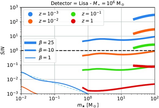
$Signal-to-noise ratio of a LISA observation of a TDE as a function of the mass of the disrupted stars for a $10^6\, \mathrm{M}_{\odot }$ BH. We show the results when the penetration factor is changed (thicker lines referring to larger β) and when the TDE occurs at a different redshift, hence at a different comoving distance (shown as different colours). For larger β, the curves are truncated at small masses, when stars penetrate twice the Schwarzschild radius of the BH. The horizontal black dashed line indicates an S/N = 1, which can be considered as an (optimistic) limit for detection, and the thin light blue dashed line guides the eye to indicate $S/N\propto m_\star ^{-0.7}$ as predicted by equation (9). Gravitational waves from β = 1 TDEs (thin lines) will not be observed by LISA; gravitational waves from TDEs of Sun-like stars will be observed up to z ∼ 10−2 for moderately β = 10 penetrating orbits (orange medium lines); at z ∼ 0.1, only gravitational waves from extreme events (β = 25 and $m_\star \gtrsim 20\, \mathrm{M}_{\odot }$; green thick line) can be observed.$

Figure 1.

Signal-to-noise ratio of a LISA observation of a TDE as a function of the mass of the disrupted stars for a |$10^6\, \mathrm{M}_{\odot }$| BH. We show the results when the penetration factor is changed (thicker lines referring to larger β) and when the TDE occurs at a different redshift, hence at a different comoving distance (shown as different colours). For larger β, the curves are truncated at small masses, when stars penetrate twice the Schwarzschild radius of the BH. The horizontal black dashed line indicates an S/N = 1, which can be considered as an (optimistic) limit for detection, and the thin light blue dashed line guides the eye to indicate |$S/N\propto m_\star ^{-0.7}$| as predicted by equation (9). Gravitational waves from β = 1 TDEs (thin lines) will not be observed by LISA; gravitational waves from TDEs of Sun-like stars will be observed up to z ∼ 10⁻² for moderately β = 10 penetrating orbits (orange medium lines); at z ∼ 0.1, only gravitational waves from extreme events (β = 25 and |$m_\star \gtrsim 20\, \mathrm{M}_{\odot }$|⁠; green thick line) can be observed.

Open in new tab Download slide

It can be somewhat surprising that sometimes, for instance when β = 1 (thin lines), S/N decreases with increasing m_⋆while equation (1) predicts that the strain increases with increasing m_⋆, i.e. larger stellar mass results in more ‘violent’ event. The reason is that f_GW (hence f_obs) also varies [equation (2)], and that the characteristic amplitude noise of LISA is not flat (see Fig. A1). To be more quantitative, we start with equation (7) in which we substitute h_GW and f_obs by their expressions from equations (1) and (3):

$$\begin{eqnarray} S/N = \frac{\pi ^{2/3} 2^{5/3} \, \mathrm{G}^{5/3}}{c^4} \times m_\star M_\bullet ^{2/3} \frac{1}{\chi (z)} \frac{f_\mathrm{GW}^{2/3}}{h_\mathrm{det}\left(\frac{f_\mathrm{GW} }{ 1+z}\right)}\, . \end{eqnarray}$$

(8)

If we further use for h_det a broken power law (h_det(f) = h_opt(f/f_opt)^−a((f/f_opt)^c + 1)^{(b + a)/c}, where f_opt is the optimal frequency of the detector, see Appendix ( A), we find:

$$\begin{eqnarray} S/N \propto \left\lbrace \begin{aligned} & m_\star ^{1+(1-3\theta)(\frac{1}{3}+\frac{a}{2})} &&\mathrm{\, if\, } f_\mathrm{GW} \ll f_\mathrm{opt}\\ & m_\star ^{1+(1-3\theta)(\frac{1}{3}-\frac{b}{2})} &&\mathrm{\, if\, } f_\mathrm{GW} \gg f_\mathrm{opt} \, . \end{aligned} \right. \end{eqnarray}$$

(9)

At this point, it is worth noting that, for β = 1, |$f_\mathrm{GW} \lesssim 10^{-3}\, \mathrm{Hz}$| for |$m_\star \gtrsim 0.01 \, \mathrm{M}_{\odot }$| such that for the different detectors (see Table 1), β = 1 TDEs are always in the regime f_GW ≪ f_opt. For the particular case of LISA (a = 1.8) shown for |$m_\star \le \, \mathrm{M}_{\odot }$| [θ = 0.8 in equation (6)] in Fig. 1, we find |$S/N \propto m_\star ^{-0.7}$| (thin light blue dashed line) in excellent agreement with the numerical estimate. Conversely, the highest possible f_GW is obtained for β = β_max:

$$\begin{eqnarray} f_\mathrm{GW,\, max} &=& \left(\frac{c^6}{32 \kappa ^3 \pi ^2 \, \mathrm{G}^2 M_\bullet ^2} \right)^{1/2}\\ && \sim 4\times 10^{-3}\, \mathrm{Hz}\, \left(\frac{\kappa }{2}\right)^{-3/2} \left(\frac{M_\bullet }{10^6\, \mathrm{M}_{\odot }}\right)^{-1} \, , \end{eqnarray}$$

(10)

which gives only |$f_\mathrm{GW,\, max} \gg f_\mathrm{opt}$| for |$\lesssim 10^4 \, \mathrm{M}_{\odot }$| BHs not considered in this study.

Table 1.

Open in new tab

Different detectors considered in this study. We indicate the optimal frequency (f_opt), strain (h_det(f_opt)), and BH mass (⁠|$M_{\bullet,\, {\rm opt}}$|⁠) of these detectors for detections of TDEs.

Detector	f_opt	h_det(f_opt)	M_{•, opt}
	Hz	10⁻²¹	\|$\, \mathrm{M}_{\odot }$\|
LISA	6 × 10⁻³	0.2	7 × 10⁵
Tianqin	0.02	7	2 × 10⁵
Alia	0.08	0.02	5 × 10⁴
Bbo	0.3	0.01	1 × 10⁴
Decigo	0.4	0.04	1 × 10⁴

Detector	f_opt	h_det(f_opt)	M_{•, opt}
	Hz	10⁻²¹	\|$\, \mathrm{M}_{\odot }$\|
LISA	6 × 10⁻³	0.2	7 × 10⁵
Tianqin	0.02	7	2 × 10⁵
Alia	0.08	0.02	5 × 10⁴
Bbo	0.3	0.01	1 × 10⁴
Decigo	0.4	0.04	1 × 10⁴

Table 1.

Open in new tab

Different detectors considered in this study. We indicate the optimal frequency (f_opt), strain (h_det(f_opt)), and BH mass (⁠|$M_{\bullet,\, {\rm opt}}$|⁠) of these detectors for detections of TDEs.

Detector	f_opt	h_det(f_opt)	M_{•, opt}
	Hz	10⁻²¹	\|$\, \mathrm{M}_{\odot }$\|
LISA	6 × 10⁻³	0.2	7 × 10⁵
Tianqin	0.02	7	2 × 10⁵
Alia	0.08	0.02	5 × 10⁴
Bbo	0.3	0.01	1 × 10⁴
Decigo	0.4	0.04	1 × 10⁴

Detector	f_opt	h_det(f_opt)	M_{•, opt}
	Hz	10⁻²¹	\|$\, \mathrm{M}_{\odot }$\|
LISA	6 × 10⁻³	0.2	7 × 10⁵
Tianqin	0.02	7	2 × 10⁵
Alia	0.08	0.02	5 × 10⁴
Bbo	0.3	0.01	1 × 10⁴
Decigo	0.4	0.04	1 × 10⁴

For a given detector (h_det known) and fixed S/N = S/N_lim, M_•, m_⋆, and β, we can solve equation (8) to obtain z_max. In Fig. 2, we show, for the particular case of LISA, and for S/N_lim = 5 and |$M_\bullet =10^6\, \mathrm{M}_{\odot }$|⁠, the value of z_max as a function of the two parameters left, m_⋆, and β. Here, we recognize that, overall, a good rule of thumb is that TDEs produced by massive stars on penetrating orbits can be detected up to higher redshift, but the details ultimately depend on the complex shape of the sensitivity curve of the gravitational wave detector (LISA in this case).

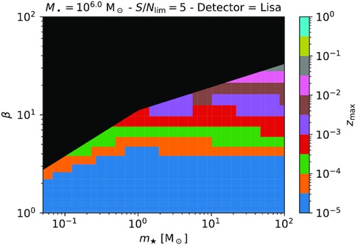
$Maximum redshift for observation with LISA of a TDE of a star with mass m⋆ on an orbit with penetration factor β around a $10^6\, \mathrm{M}_{\odot }$ BH assuming detection if S/N ≥ 5. The black region indicates when the orbit plunges directly toward the BH (rT/β < 2rSch). Conclusions are identical to that of Fig. 1.$

Figure 2.

Maximum redshift for observation with LISA of a TDE of a star with mass m_⋆ on an orbit with penetration factor β around a |$10^6\, \mathrm{M}_{\odot }$| BH assuming detection if S/N ≥ 5. The black region indicates when the orbit plunges directly toward the BH (r_T/β < 2r_Sch). Conclusions are identical to that of Fig. 1.

Open in new tab Download slide

In order to understand the dependency of z_max with M_•, we fix m_⋆ and S/N_lim, and we solve equation (8) across all the possible β. We show the results in Fig. 3 (light thick lines), where we explore different stellar masses m_⋆ and S/N_lim for LISA (left-hand panel), as well as for future gravitational waves detectors but with fixed |$m_\star =\, \mathrm{M}_{\odot }$| and S/N_lim = 1 (right-hand panel). Here, the exact shape of the sensitivity curve appears even more clearly: LISA is optimal around |$10^6\, \mathrm{M}_{\odot }$| BHs.

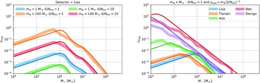
$Left: Maximum redshift at which a TDE can be detected with LISA as a function of the mass of the BH around which the TDE occurs. We explore different stellar masses and thresholds for the signal-to-noise ratio (colours) and show the results of a numerical search (thick light lines) and from equation (12) (thin dark lines). LISA is optimal for a detection around a $10^6\, \mathrm{M}_{\odot }$ BH. Right: Same, but for $m_\star =1\, \mathrm{M}_{\odot }$ and S/Nlim = 1 and different detectors (colours). The generation of gravitational waves detectors following LISA will be able to detect TDEs from intermediate mass BHs up to cosmological redshifts.$

Figure 3.

Left: Maximum redshift at which a TDE can be detected with LISA as a function of the mass of the BH around which the TDE occurs. We explore different stellar masses and thresholds for the signal-to-noise ratio (colours) and show the results of a numerical search (thick light lines) and from equation (12) (thin dark lines). LISA is optimal for a detection around a |$10^6\, \mathrm{M}_{\odot }$| BH. Right: Same, but for |$m_\star =1\, \mathrm{M}_{\odot }$| and S/N_lim = 1 and different detectors (colours). The generation of gravitational waves detectors following LISA will be able to detect TDEs from intermediate mass BHs up to cosmological redshifts.

Open in new tab Download slide

All this can be understood as follows. Starting with equation (8) and using that, for z ≪ 1, we can approximate χ ∼ cz/H₀ (H₀ is the Hubble constant), we have:

$$\begin{eqnarray} z \underset{z \ll 1}{\sim }\frac{\pi ^{2/3} 2^{5/3} \, \mathrm{G}^{5/3} H_0}{c^5} \times \frac{m_\star M_\bullet ^{2/3}}{S/N} \frac{f_\mathrm{GW}^{2/3}}{h_\mathrm{det}\left(f_\mathrm{GW} \right)}. \end{eqnarray}$$

(11)

If |$f_\mathrm{GW,\, max} \ge f_\mathrm{opt}$|⁠, then there exists β for which h_det(f_GW) = h_opt, and as h_det is a steep function of f, this is where the maximal z is obtained. In the other situation, if |$f_\mathrm{GW,\, max} \le f_\mathrm{opt}$|⁠, then, given the U shape of h_det, the maximal z is obtained for |$f_\mathrm{GW,\, max}$|⁠. Overall, equation (11) giving the maximum redshift can be wrapped up as:

$$\begin{eqnarray} z_\mathrm{max} &=& 0.01 \left(\frac{m_\star }{\, \mathrm{M}_{\odot }}\right)^{} \left(\frac{M_\bullet }{10^6\, \mathrm{M}_{\odot }}\right)^{2/3} \\ &&\times \,\, S/N_{{\lim }}^{-1} \left(\frac{f_\star }{10^{-2}\, \mathrm{Hz}}\right)^{2/3} \left(\frac{h_\mathrm{det}(f_\star)}{10^{-21}}\right)^{-1}, \end{eqnarray}$$

(12)

where

$$\begin{eqnarray} f_\star = \mathrm{min}\left(4\times 10^{-3}\, \mathrm{Hz}\, \left(\frac{\kappa }{2}\right)^{-3/2} \left(\frac{M_\bullet }{10^6\, \mathrm{M}_{\odot }} \right)^{-1} , f_\mathrm{opt}\right) \, . \end{eqnarray}$$

(13)

We conclude that |$z_\mathrm{max}\propto m_\star S/N_{{\lim }}^{-1}$| is always true: more massive stars can be detected farther away. However, for BHs with |${f_\mathrm{GW,\, max} \ge f_\mathrm{opt}}$| (BHs lighter than |$M_{\bullet ,\, {\rm opt}}$|⁠, see Table 1), we have |$z_\mathrm{max}\propto ~M^{2/3}_\bullet$|⁠, and for |${f_\mathrm{GW,\, max} \lt f_\mathrm{opt}}$| (‘massive’ BHs), z_max decreases faster than |$M^{-1/3}_\bullet$|⁠: even though the signals are stronger for more massive BHs, there exists an optimal BH mass for detection given by |${f_\mathrm{GW,\, max}(M_\bullet)=f_\mathrm{det}}$|⁠. For LISA, this optimal mass is |$M_{\bullet ,\, {\rm opt}}\sim 10^6\, \mathrm{M}_{\odot }$|⁠, and this is why z_max peaks at this value in Fig. 3 (left). We also show in Fig. 3 the results of equation (12) (thin lines), apart when z_max ∼ 1 and our hypothesis z ≪ 1 is not correct anymore, the numerical estimate and equation (12) are in excellent agreement.

Overall, LISA can realistically detect TDEs only up to z ∼ 0.01 − 0.1 (depending on m_⋆ and S/N_lim), but the next-generation detectors will be able to detect TDEs around intermediate-mass BHs up to cosmological redshifts. In all cases, detectors are most sensible to BHs for which the Keplerian frequency around the critical radius for direct plunge (κ × r_Sch) is the same as the optimal frequency of the detector, about |$10^6\, \mathrm{M}_{\odot }$| for LISA (see Table 1).

2.2 Electromagnetic counterpart

TDEs are very luminous electromagnetic sources bright both in the X-ray (e.g. Saxton et al. 2020) and in the optical (e.g. van Velzen et al. 2020a) part of the spectrum. With the aim of exploring possible TDEs observed as multimessenger sources, we estimate, using observationally motivated models, the electromagnetic luminosity of TDEs. We begin with the optical emission in Section 2.2.1 and then move to the X-ray emission in Section 2.2.4.

2.2.1 Optical emission

Formalism. The origin of the optical emission is still debated: while some groups believe that it is caused by shocks during the circularization process (e.g. Lodato 2012; Piran et al. 2015; Shiokawa et al. 2015), others believe that it is sourced by the accretion luminosity reprocessed in the expanding outflow (e.g. Lodato & Rossi 2011; Dai et al. 2018; Roth & Kasen 2018). Discussion about the origin of the optical component is beyond the scope of this paper, and we instead adopt an observational-driven approach. We assume that the optical emission of TDEs can be well modelled with a blackbody with temperature |$T_{\rm opt}=3\times 10^4\, \text{K}$| (mean temperature from table 3 of Wevers et al. 2017 but see also van Velzen et al. 2020b), and a luminosity equals to the Eddington limit:

$$\begin{eqnarray} L_{\rm Edd} = 3\times 10^4 \text{L}_{\odot }\left(\frac{M_{\bullet }}{M_{\odot }}\right) \, , \end{eqnarray}$$

(14)

where L_⊙ is the luminosity of the Sun. It should be noted that not all observed TDEs emit up to Eddington luminosity (e.g. Hung et al. 2017). Furthermore, in our vast parameter space, the Eddington luminosity can sometime exceed the luminosity at peak [e.g. Evans & Kochanek 1989; Stone, Sari & Loeb 2013; equation (24) of Stone & Metzger 2016]; for this reason, the final adopted luminosity is:

$$\begin{eqnarray} L&=&L_{\rm Edd} \times {\rm min}\left(1; 133 \left(\frac{M_\bullet }{10^6\, \mathrm{M}_{\odot }}\right)^{-3/2} \left(\frac{m_\star }{\, \mathrm{M}_{\odot }}\right)^{2}\left(\frac{r_\star }{\, \mathrm{R}_{\odot }}\right)^{-3/2}\right) , \\ \end{eqnarray}$$

(15)

where we adopted a constant radiative efficiency of 0.1.

This allows to write the spectral flux density (appropriately redshifted as in appendix A of Roth et al. 2020a):

$$\begin{eqnarray} F_{\rm opt}(\lambda)&=& \frac{(1+z)^2}{\chi (z)^2}\times \frac{2hc^2}{\lambda ^5}\\ &&\times \frac{R^2_{\rm opt}}{\exp \left(hc(1+z)/\lambda k_\mathrm{ B} T_{\rm opt}\right)-1}, \end{eqnarray}$$

(16)

where λ is wavelength in the observer frame; h, k_B, and σ_S are the Planck, the Boltzmann, and the Stefan constants, respectively; and we defined the typical blackbody radius of emission (R_opt) from the Stefan–Boltzmann law:

$$\begin{eqnarray} R_{\rm opt} = \sqrt{\frac{L}{4 \pi \sigma _S T^4_{\rm opt}}}\, . \end{eqnarray}$$

(17)

From all this, the G magnitude associated to the flux is

$$\begin{eqnarray} M_G = -2.5 \mathrm{log}_{10}\Bigg (9\times \left(\frac{\lambda _{\rm G}}{{\rm \mathring{\rm A}}}\right)^2\times \frac{F_{\rm opt}(\lambda _{\rm G})}{\text{erg}\, \text{cm}^{-2}\text{s}^{-1}{\rm \mathring{\rm A}}^{-1}}\Bigg), \end{eqnarray}$$

(18)

where |$\lambda _{\rm G}\sim 464\, \text{nm}$| is the central wavelength of the G band.

Note that for L = L_Edd (most cases in our parameter space), we can approximate equation (18) for small z similarly to Section 2.1.2 to obtain the following simple expression:

$$\begin{eqnarray} M_G \sim 28 -2.5\mathrm{log}_{10}\left(\frac{M_\bullet }{10^6\, \mathrm{M}_{\odot }} \right) + 5\mathrm{log}_{10}(z) \, . \end{eqnarray}$$

(19)

Under the observationally motivated assumption L = L_Edd, the magnitude of a TDE solely depends on the mass of the BH and the cosmological distance.

Multimessenger TDEs: For a TDE with given properties, we can now estimate what the maximum redshift is at which it can be observed with a gravitational wave detector [equation (12)] as well as the G magnitude of this event [equation (18)]. In order to address which events can be detected both in the electromagnetic and the gravitational spectrum, we can estimate the G magnitude in the most pessimistic scenario (M_{G, lim}): when the TDE occurs at z_max.

We show in Fig. 4M_{G, lim} as a function of M_• for TDEs of |$10\, \mathrm{M}_{\odot }$| stars and assuming that events can be gravitationally detected with S/N_lim = 5. This can easily be generalized to any m_⋆ and S/N_lim; combining the approximate expressions for M_G [equation (19)] and z_max [equation (12)], one finds:

$$\begin{eqnarray} M_{G, {\rm lim}} &=& 18+5\mathrm{log}_{10}\left(\frac{m_\star }{\, \mathrm{M}_{\odot }} \right)-5\mathrm{log}_{10}\left(S/N_{\lim } \right)\\ &&+\,\, \frac{5}{6}\mathrm{log}_{10}\left(\frac{M_\bullet }{10^6\, \mathrm{M}_{\odot }} \right)\\ &&+\,\,5\mathrm{log}_{10}\left(\left(\frac{f_\star }{10^{-2}\, \mathrm{Hz}}\right)^{2/3}\left(\frac{h_{\rm det}(f_\star)}{10^{-21}}\right)^{-1} \right) \, . \end{eqnarray}$$

(20)

Any gravitational detection with the two upcoming interferometers LISA and Tianqin should be associated with a maximum M_{G, lim} magnitude ≲ 20, even detectable with current wide field facilities (YSE and ZTF M_G limit is 21.5, see Jones et al. 2020). As a consequence, if there is a detection of a TDE through gravitational waves, there should be a detection of its electromagnetic counterpart. However, future-generation detectors may see gravitational waves that are not observed in the optical counterparts: there will be orphans. Since for BHs lighter than the optimal mass for gravitational waves detection (⁠|$M_{\bullet ,\, {\rm opt}}$|⁠, see Table 1), M_{G, lim}increases with the mass of the BH [as 5/6 × log₁₀M_•, see equation (20)], while it decreases for more massive BHs (faster than −5/2 × log₁₀M_•, given the expression of f_⋆ in this regime), these orphans are most likely to be powered by BHs with a mass around |$M_{\bullet ,\, {\rm opt}}$|⁠.

Figure 4.

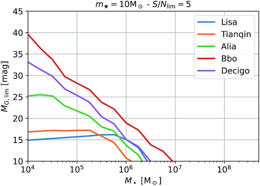
Gmagnitude as a function of M_• for a TDE of a m_⋆ = 10 star occurring at the maximum observable redshift with different gravitational wave detectors.

Open in new tab Download slide

2.2.2 X-ray emission

Formalism. The origin of the X-ray emission is thought to be associated to the inner parts of an accretion disc (e.g. Ulmer 1999; Lodato & Rossi 2011). We adopt a similar method as in Section 2.2.1, but instead of fixing the temperature, we fix the blackbody radius at the circularization radius of the stellar debris:

$$\begin{eqnarray} R_{\rm x}=\frac{2r_{\rm T}}{\beta } \, , \end{eqnarray}$$

(21)

and, similarly to the optical case (van Velzen et al. 2016), we assume that the luminosity equals the Eddington limit capped at the luminosity at peak [equation (15)]. This allows to estimate the spectral flux density [equation (16)], which can be integrated in the 0.3–10 keV band in order to obtain the X-ray flux.

Multimessenger TDEs. Similarly to Section 2.2.1, we estimate the X-ray flux in the pessimistic regime of a TDE occurring at the maximum redshift at which it can be observed with a gravitational wave detector. Note that, contrary to the optical emission, this flux depends on the mass of the star not only through z_max but also through R_X. Note also that the value of β matters, and to estimate the flux, we take β for which f_GW = f_⋆, i.e. such that the event is observable at z_max.

We show in Fig. 5 the X-ray flux as a function of M_•. We also mark the optimistic flux limit of Lynx (⁠|$10^{-19} \mathrm{\, erg}\, \mathrm{cm}^{-2} \, \mathrm{s}^{-1}$|⁠; The Lynx Team 2018), but similar conclusions can be reached for eROSITA (flux limit of |$10^{-14} \mathrm{\, erg}\, \mathrm{cm}^{-2} \, \mathrm{s}^{-1}$|⁠; Merloni et al. 2012). In the upper plot, we focus on the case of LISA varying m_⋆ (colours). We find that most TDEs that LISA may reveal through gravitational waves should be detectable in the X-ray. Similarly to the optical counterpart, we find that, in general, if we consider more massive stars, the X-ray counterpart is fainter as the maximum redshift is larger. In the lower plot, we show the results for future gravitational wave detectors, with the same conclusions.

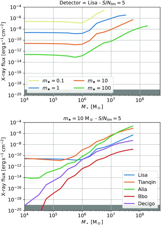
$X-ray flux as a function of M•. Top: Case of LISA, we vary the total luminosity (varying the fraction of the Eddington limit, line style) and the mass of the disrupted star (colour, low-mass stars curves are truncated for large BH masses, when stars penetrate the Scwhazschild radius before being disrupted). Bottom: Case of future detectors (colours). In both cases, the Lynx limit is indicated in black.$

Figure 5.

X-ray flux as a function of M_•. Top: Case of LISA, we vary the total luminosity (varying the fraction of the Eddington limit, line style) and the mass of the disrupted star (colour, low-mass stars curves are truncated for large BH masses, when stars penetrate the Scwhazschild radius before being disrupted). Bottom: Case of future detectors (colours). In both cases, the Lynx limit is indicated in black.

Open in new tab Download slide

3 TDE RATES

As shown in Section 2, the detectability of a TDE, both in gravitational and electromagnetic waves, depends on the mass of the BH as well as the properties of the disrupted star (mass and radius) and on the pericentre of its orbit. In order to obtain the rate of observable events, we compute the total rate as a function of these parameters in one single galaxy in Section 3.1, and we then generalize to a population of galaxies in Section 3.2.

3.1 Single galaxy

In this section, for a given galaxy with a central BH, we derive the TDE rate at which stars with a given mass and pericentre penetrate the tidal radius and are disrupted. A summary of the loss cone dynamics is given in Section 3.1.1; as the rate depends on the structure of the galaxy (e.g. density profile), we describe our assumptions in Section 3.1.2, and we compare our results with previous studies in Section 3.1.5.

3.1.1 Loss cone dynamics

For a spherically symmetric bath formed by a monochromatic population of stars m_bg, we classically (Binney & Tremaine 1987; Merritt 2013; Stone & Metzger 2016) define the absolute value of the specific energy, E, the specific angular momentum J, the specific angular momentum of a circular orbit at a given energy, J_c(E), their ratio |$R=J^2/J^2_\mathrm{ c}$|⁠, the radial period, P(E),² and the mean-R distribution function f(E).

The flux of stars with a given energy and impact parameter that diffuse through 2-body interactions within an angular momentum limit R_LC is given by equations (4.90–4.94) of Strubbe 2011, and variable change):

$$\begin{eqnarray} \frac{\mathrm{d}^2 \Gamma }{\mathrm{d}E \mathrm{d}\ln \beta } &=& \frac{8 \pi ^2 \, \mathrm{G}M_\bullet r_T}{\beta } \frac{f(E)}{1+q^{-1}\xi \ln \left(R^{-1}_\mathrm{LC}\right)} \\ &&\times \left[1-2\sum _{m=1}^\infty \frac{e^{-\alpha ^2_m q/4}}{\alpha _m} \frac{J_0\left(\alpha _m \beta ^{-1/2}\right)}{J_1(\alpha _m)} \right] \end{eqnarray}$$

(22)

$$\begin{eqnarray} \xi = 1 - 4 \sum _{m=1}^\infty \frac{e^{-\alpha ^2_m q/4}}{\alpha ^2_m} \end{eqnarray}$$

(23)

$$\begin{eqnarray} q(E, m_\star , m_\mathrm{bg}) &=& \frac{P \overline{\mu }(E, m_\star , m_\mathrm{bg})}{R_\mathrm{LC}}\, , \end{eqnarray}$$

(24)

where q is the loss cone filling factor corresponding to the relative change of R to R_LC per orbit; |$\overline{\mu }(E,m_\mathrm{bg},m_\star)$| is the orbit averaged diffusion coefficient in R corresponding to the inverse of the typical time to change R by order unity (equation [18] of Merritt 2013, equation [11] of Stone & Metzger 2016); J_k are the Bessel functions of first kind of order k; and α_m is the m-th zero of J₀.

We define the TDE rate as the rate at which stars diffuse within the angular momentum limit such that they are doomed to enter the disruption zone on a time-scale of the orbital period, that is:

$$\begin{eqnarray} R_\mathrm{LC}(E, m_\star) \sim \frac{4 E r_\mathrm{ T}}{\, \mathrm{G}M_\bullet } \ll 1 \, , \end{eqnarray}$$

(25)

where we have used that |$E \ll \, \mathrm{G}M_\bullet /r_\mathrm{ T}$|⁠, as most stars arrive on eccentric orbit with semimajor axis much larger than r_T.

If we consider now a stellar population described by a mass function ϕ, then, in principle, (i) for a given test mass m_⋆, the diffusion caused by a multispecies stellar background should differ from the simple monochromatic case; and (ii) different test particles with different masses should diffuse differently. However, by a happy coincidence (Magorrian & Tremaine 1999, summary in Appendix B), for a stellar population, the resulting rate happens to be the same as if the distribution was made by a monochromatic bath with mass |$m_\mathrm{bg}=\langle m_\star ^2 \rangle ^{1/2}$|⁠, where |$\langle m_\star ^2 \rangle = \int m^2\phi (m)\mathrm{d}m$| is the root-mean-square of the mass of a star. Obviously, this is not true anymore when ϕ depends on the position: for instance, if there is mass segregation that brings more massive objects to the centre, or close enough to the BH so that more massive stars are disrupted. We neglect these processes in what follows. Consequently, the rate at which test particles diffuse within some angular momentum limit can be obtained using equation (22) with |$m_\mathrm{bg}=\langle m_\star ^2 \rangle ^{1/2}$|⁠.

In order to obtain the rate for a given mass, one has to consider that only a fraction ϕ(m_⋆)dm_⋆ of test particles have the mass m_⋆, and that the boundary for disruption (R_LC) depends on m_⋆; this yields:

$$\begin{eqnarray} \frac{\mathrm{d}^2 \Gamma }{\mathrm{d}\ln m_\star \mathrm{d}\ln \beta } &=& \frac{8 \pi ^2 \, \mathrm{G}M_\bullet r_T}{\beta } \phi (m_\star)m_\star \\ &&\times \,\,\int _{0}^{\, \mathrm{G}M_\bullet / r_T} \mathcal {G}(E,\beta ,m_\star) \mathrm{d}E \end{eqnarray}$$

(26)

$$\begin{eqnarray} \mathcal {G}(E,\beta ,m_\star) &=& \frac{f(E)}{1+q^{-1}\xi \ln (R^{-1}_\mathrm{LC})} \\ &&\times \left[1-2\sum _{m=1}^\infty \frac{e^{-\alpha ^2_m q/4}}{\alpha _m} \frac{J_0\left(\alpha _m \beta ^{-1/2}\right)}{J_1(\alpha _m)} \right] \end{eqnarray}$$

(27)

$$\begin{eqnarray} \xi = 1 - 4 \sum _{m=1}^\infty \frac{e^{-\alpha ^2_m q/4}}{\alpha ^2_m} \end{eqnarray}$$

(28)

$$\begin{eqnarray} q(E, m_\star) &=& \frac{P(E) \overline{\mu }(E, \langle m^2_\star \rangle ^{1/2})}{R_\mathrm{LC}} \, , \end{eqnarray}$$

(29)

where the upper bound in the integral comes from that orbits with higher E are within the tidal radius. We note that this upper bound on E is in apparent contradiction with equation (25), but we have checked that the integral is independent of the upper value chosen, i.e., the rate is not dominated by the energy range near |$\, \mathrm{G}M_\bullet / r_\mathrm{ T}$|⁠.

From equation (26), we can obtain the total TDE rate (Γ) around a particular BH as:

$$\begin{eqnarray} \Gamma = \int _{m_\star =m_{\star ,\min }}^{m_{\star ,\max }} \int _{\beta =0}^{\beta _{\max }} \frac{\mathrm{d}^2 \Gamma }{\mathrm{d}\ln m_\star \mathrm{d}\ln \beta } \mathrm{d}\ln m_\star \mathrm{d}\ln \beta \, , \end{eqnarray}$$

(30)

where m_{⋆, min} and m_{⋆, max} are the boundaries of the stellar mass function (see following section).

3.1.2 Stellar properties around the BH

Stellar density function.In general, the estimate of f and q requires numerical integration (for instance, using PhaseFlow; Vasiliev 2017; Pfister et al. 2019b, 2020a; Pestoni et al. 2021) or approximations (Wang & Merritt 2004; Pfister et al. 2020b). However, we further assume that the stellar density profile surrounding the BH is a power law:

$$\begin{eqnarray} \rho (r) &=& \rho _0\left(\frac{r}{r_\mathrm{inf}} \right)^{-\alpha } , \end{eqnarray}$$

(31)

where r_inf is the influence radius of the BH, corresponding to the radius encompassing a stellar mass equal to that of the BH (which also defines ρ₀). In this situation, f and q can be obtained analytically within r_inf (Magorrian & Tremaine 1999; Strubbe 2011; Merritt 2013; Stone & Metzger 2016), when the potential is dominated by the BH, as:

$$\begin{eqnarray} {f}(E) &=& \left(2\pi \sigma ^2_\mathrm{inf}\right)^{-3/2}\frac{\rho _0}{\langle m_\star \rangle } \frac{\gamma (\alpha +1)}{\gamma (\alpha -1/2)} \left(\frac{E}{\sigma ^2_\mathrm{inf}} \right)^{\alpha -3/2} \end{eqnarray}$$

(32)

$$\begin{eqnarray} q(E,m_\star) &=& \nu \left(\frac{E}{\sigma ^2_\mathrm{inf}} \right)^{\alpha -4} \end{eqnarray}$$

(33)

$$\begin{eqnarray} \nu (m_\star) &=& \frac{8\sqrt{\pi }}{3}(3-\alpha) \frac{\gamma (\alpha +1)}{\gamma (\alpha -1/2)} \left[ \frac{5}{32(\alpha -\frac{1}{2})} \right.\\ &&+\left. \frac{3I_B\left(\frac{1}{2},\alpha\right)-I_B\left(\frac{3}{2},\alpha\right)}{4\pi } \right] \left(\frac{\, \mathrm{G}\langle m_\star ^2 \rangle }{\sigma ^2_\mathrm{inf} \langle m_\star \rangle r_T(m_\star)} \right) \ln \Lambda, \\ \end{eqnarray}$$

(34)

where |$\sigma _\mathrm{inf}=(\, \mathrm{G}M_\bullet /r_\mathrm{inf})^{1/2}$| is the velocity dispersion at r_inf; 〈m_⋆〉 = ∫mϕ(m)dm is the mean stellar mass; ln Λ = ln (0.4M_•/〈m_⋆〉) is the Coulomb logarithm (Spitzer & Hart 1971); γ is the Euler Gamma function;³ and we define I_B as:

$$\begin{eqnarray} I_\mathrm{ B}\left(\frac{n}{2},\alpha\right) &=& \int _0^1t^{-\frac{n+1}{2}}(1-t)^{3-\alpha } \mathrm{ B}\left(t,\frac{n}{2},\alpha -\frac{1}{2}\right) \mathrm{d}t \, , \end{eqnarray}$$

(35)

where B the incomplete Euler Beta function.⁴

In order to reduce the dimensionality of the problem, we assume that the density profile is an isothermal sphere [α = 2 in equation (31)]:

$$\begin{eqnarray} \rho (r) &=& \frac{\sigma ^2}{2\pi \, \mathrm{G}r^2} \end{eqnarray}$$

(36)

$$\begin{eqnarray} r_\mathrm{inf} &=& \frac{\, \mathrm{G}M_\bullet }{2 \sigma ^2} \end{eqnarray}$$

(37)

$$\begin{eqnarray} \sigma _\mathrm{inf} &=& \sqrt{2}\sigma \, , \end{eqnarray}$$

(38)

where σ is the velocity dispersion of the galaxy and is such that the BH lies on the M_• − σ relation (Merritt & Ferrarese 2001):

$$\begin{eqnarray} \frac{\sigma }{\, \mathrm{km}\, \mathrm{s}^{-1}} = 68 \left(\frac{M_\bullet }{10^6\, \mathrm{M}_{\odot }} \right)^{0.22} \, . \end{eqnarray}$$

(39)

The assumption of an isothermal sphere lying on the M_• − σ relation is clearly a simplification of reality, as galaxies exhibit different shapes (e.g. Lauer et al. 2007) and are not uniquely defined by their BH mass (there is scatter in the relation, e.g. Kormendy & Ho 2013). One possibility to overcome this issue would be to use a mock catalogue (e.g. Pfister et al. 2020a; Chen, Yu & Lu 2020), but (i) this is beyond the scope of this study which aims only at providing trends and orders of magnitude on the gravitationally observed TDE rates, and (ii) these mock catalogues are constructed from real observations for which the structure within the influence radius (the relevant region for TDE rates estimates) is usually poorly resolved for BHs with |$M_\bullet \lesssim 10^6 \, \mathrm{M}_{\odot }$| (Pechetti et al. 2019; Sánchez-Janssen et al. 2019). This said, we note that the isothermal sphere lying on the M_• − σ has been widely used in Astronomy (e.g. Volonteri, Haardt & Madau 2003; Barausse et al. 2020), including TDE studies for which it has shown to reproduce well observations (Wang & Merritt 2004; Kochanek 2016b). We also note that the use of the M_• − σ relation of Merritt & Ferrarese (2001) among the different observationally found (e.g. Kormendy & Ho 2013) has little effects on the rate, as shown by section 3.2 of Kochanek (2016b).

Stellar mass function. In order to take into account that stars can have a variety of masses, which will produce differences in the strain, we assume that the stellar population follows the usual Kroupa stellar mass function (Kroupa 2001):

$$\begin{eqnarray} \phi (m_\star) = \phi _0 \left\lbrace \begin{aligned} & \left(\frac{m_\star }{0.5 \, \mathrm{M}_{\odot }} \right)^{-1.3} &&\mathrm{\, for\, } m_\mathrm{\star ,\, min} \le m_\star \le 0.5 \, \mathrm{M}_{\odot }\\ & \left(\frac{m_\star }{0.5 \, \mathrm{M}_{\odot }} \right)^{-2.3} &&\mathrm{\, for\, }0.5 \, \mathrm{M}_{\odot }\le m_\star \le m_\mathrm{\star ,\, max} &\\ &0 &&\mathrm{\, else} \, , \end{aligned} \right. \end{eqnarray}$$

(40)

where ϕ₀ is such that ∫ϕ(m)dm = 1. Our fiducial model is for |$(m_\mathrm{\star ,\, min}, m_\mathrm{\star ,\, max})=(0.08,10)\, \mathrm{M}_{\odot }$|⁠, that is the stellar population is old enough so that massive stars have gone through supernovae (similarly to Magorrian & Tremaine 1999; Stone & Metzger 2016), but we explore populations with |$m_\mathrm{\star ,\, max}$| ranging from |$2.5\, \mathrm{M}_{\odot }$| to |$100\, \mathrm{M}_{\odot }$|⁠. For comparison with previous studies, we also consider the monochromatic Solar population |$\phi (m_\star)= \delta (m_\star -\, \mathrm{M}_{\odot })$|⁠, where δ is the delta Dirac function.

The use of the Kroupa initial mass function among others (Salpeter 1955; Chabrier 2003) is an arbitrary choice, but Stone & Metzger (2016) have shown that the TDE rates depend more on the boundaries (⁠|$m_\mathrm{\star ,\, min}$| and |$m_\mathrm{\star ,\, max}$|⁠) than on the mass function chosen. While it would be interesting to also vary the initial mass function, it is unfortunately impossible to explore all the possibilities in a finite and comprehensible paper.

For a given BH with mass M_•, we now have a unique stellar density profile and distribution function (f). If we further assume a stellar mass function (ϕ), we can estimate all the different terms in equation (26) to obtain the TDE rate for a given stellar mass (m_⋆) and impact parameter (β).

3.1.3 Summary

Analytical considerations. As noted by Magorrian & Tremaine (1999) and Stone & Metzger (2016), if the TDE rate is dominated by the ‘empty loss cone’ regime (or ‘diffusive’ regime with q ≪ 1), then the total rate scales as |$\Gamma \propto \langle m_\star ^2 \rangle / \langle m_\star \rangle ^2$| (⁠|$\langle m_\star ^2 \rangle /\langle m_\star \rangle$| from |$\overline{\mu }$| and 1/〈m_⋆〉 from f). As we also take into consideration that low-mass stars can be swallowed whole, we have to remove the fraction f_• of stars with m_⋆ ≤ m_{⋆, •}, where m_{⋆, •} is solution to β_max = 1 (equation [4]). In the end, the total rate scales as:

$$\begin{eqnarray} \frac{\Gamma }{\Gamma _\odot } = f_\bullet \frac{ \langle m_\star ^2 \rangle }{ \langle m_\star \rangle ^2} \, , \end{eqnarray}$$

(41)

where |$f_\bullet = \int _{m_{\star , \bullet }}^{m_{\star , \max }} \phi (u)\mathrm{d}u$|⁠, and Γ_⊙ is the TDE rate for a monochromatic solar population.

We show in Fig. 6m_{⋆, •} as a function of the BH mass. Given our minimum stellar mass considered of 0.08 |$\, \mathrm{M}_{\odot }$|⁠, BHs with |$M_\bullet \lesssim 10^7\, \mathrm{M}_{\odot }$| can disrupt all stars; for more massive BHs, low-mass stars are gradually removed such that only massive stars can be disrupted, and for BHs with a mass above |$\sim 2 \times 10^8\, \mathrm{M}_{\odot }$|⁠, even most massive stars with |$m_\star \sim 100\, \mathrm{M}_{\odot }$| are swallowed whole. As a consequence, rather independently on the maximum boundary |$m_{\star ,\, \max }$|⁠, the fraction of stars that can be disrupted is f_• = 1 for |$M_\bullet \lesssim 10^7 \, \mathrm{M}_{\odot }$| and gradually drops to 0 for |$M_\bullet \gtrsim 2\times 10^8 \, \mathrm{M}_{\odot }$| passing by 0.77 and 0.16 for M_• = 10⁷ and |$10^{7.5}\, \mathrm{M}_{\odot }$|⁠.

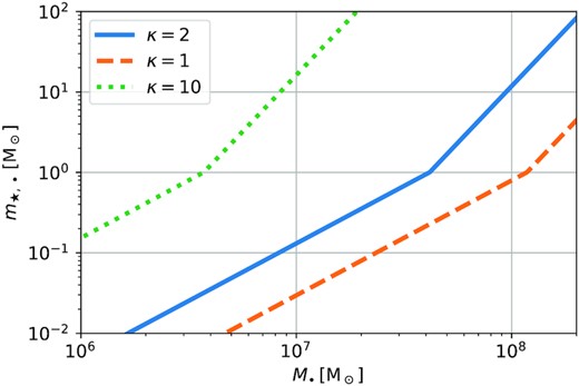
$Minimum stellar mass that can produce a TDE as a function of the mass of the BH for different κ (the critical radius for direct plunge, see Section 2.1.1). For the κ = 2 case, BHs with $M_\bullet \lesssim 10^7\, \mathrm{M}_{\odot }$ can disrupt all stars; for more massive BHs, low-mass stars are gradually removed such that only massive stars can be disrupted, and for BHs with a mass above $\sim 2 \times 10^8\, \mathrm{M}_{\odot }$, even most massive stars with $m_\star \sim 100\, \mathrm{M}_{\odot }$ are swallowed whole.$

Figure 6.

Minimum stellar mass that can produce a TDE as a function of the mass of the BH for different κ (the critical radius for direct plunge, see Section 2.1.1). For the κ = 2 case, BHs with |$M_\bullet \lesssim 10^7\, \mathrm{M}_{\odot }$| can disrupt all stars; for more massive BHs, low-mass stars are gradually removed such that only massive stars can be disrupted, and for BHs with a mass above |$\sim 2 \times 10^8\, \mathrm{M}_{\odot }$|⁠, even most massive stars with |$m_\star \sim 100\, \mathrm{M}_{\odot }$| are swallowed whole.

Open in new tab Download slide

We show in Fig. 7, for different BH masses (colours), the ratio of the TDE rate with respect to the one of a monochromatic solar population. This ratio is shown as a function of the maximum stellar mass |$m_{\star ,\, \max }$| in the stellar mass function. The results are presented for our model obtained using equation (30) (solid lines) as well as in the empty loss cone regime using equation (41) (dashed line). The scaling with the empty loss cone is overall quite good. Yet, in the low-mass BH regime (⁠|$10^{4}-10^5\, \mathrm{M}_{\odot }$|⁠, blue and orange), there is a mismatch between the empty loss cone ratio and the ‘real’ ratio. In the higher-mass BH regime (⁠|$10^{7.5}\, \mathrm{M}_{\odot }$|⁠, red), the agreement is better. This is in agreement with Stone & Metzger (2016), who find that the fraction of TDEs in the empty loss cone regime dominates in the high-mass BH end but not for low-mass BH.

Figure 7.

Ratio, for different BH masses (colours), of the TDE rate for a realistic stellar population over the TDE rate for a monochromatic solar population. The higher the BH mass, the better the matching between our model [solid line, equation (30)] and the empty loss cone model [dashed line, equation (41)]: in the low-mass end, the rate is not dominated by the empty loss cone regime.

Open in new tab Download slide

Comparison with previous results. We show in Fig. 8 the TDE rate Γ [equation (30)] as a function of M_• for our model (solid lines) and from previous studies (dashed lines). For our model, we perform the exercise for the three different stellar mass functions (shown as different colours). Our results with a monochromatic Sun-like population (solid blue) are in excellent agreement with those from Wang & Merritt (2004) (dashed pink): this was expected as both models use similar assumptions, but this is a nice test to confirm the validity of our model, of our numerical implementation, and of our results. As discussed in the paragraph above, and similarly to Magorrian & Tremaine (1999) or Stone & Metzger (2016), we find an enhancement of the rate when we extend the stellar mass function. Finally, we also note that the TDE rates sharply drop to 0 at |$M_\bullet \sim 10^8\, \mathrm{M}_{\odot }$| for a monochromatic Sun-like population and smoothly decreases starting from few |$10^7\, \mathrm{M}_{\odot }$| for a more realistic stellar population. This is due to that low-mass stars (see Fig. 6) are gradually removed when we shift towards more massive BHs (see also fig. 4 of Kochanek 2016b).

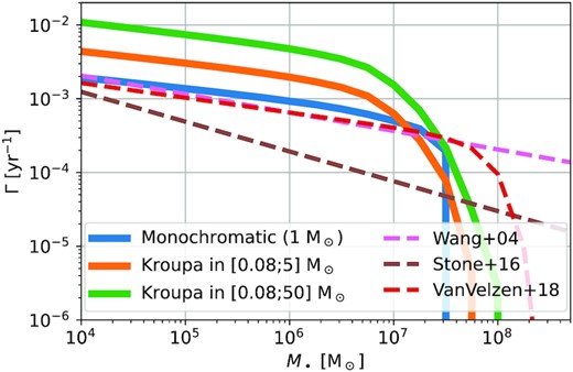
$TDE rate as a function as the mass of the central BH. We show the results from our study (thick lines) and from previous works (dashed lines; Wang & Merritt 2004; Stone & Metzger 2016; van Velzen 2018). Rates are increased if we change the stellar mass function (at first order, it scales with $\langle m_\star ^2 \rangle /\langle m_\star \rangle ^2$; Magorrian & Tremaine 1999; Stone & Metzger 2016), but our results for a monochromatic Sun-like population (blue line) are in excellent agreement with previous studies. When more massive stars are included, TDEs can occur around more massive BHs, which explains why the drop shifts towards heavier BH masses when the stellar mass function is extended.$

Figure 8.

TDE rate as a function as the mass of the central BH. We show the results from our study (thick lines) and from previous works (dashed lines; Wang & Merritt 2004; Stone & Metzger 2016; van Velzen 2018). Rates are increased if we change the stellar mass function (at first order, it scales with |$\langle m_\star ^2 \rangle /\langle m_\star \rangle ^2$|⁠; Magorrian & Tremaine 1999; Stone & Metzger 2016), but our results for a monochromatic Sun-like population (blue line) are in excellent agreement with previous studies. When more massive stars are included, TDEs can occur around more massive BHs, which explains why the drop shifts towards heavier BH masses when the stellar mass function is extended.

Open in new tab Download slide

Fraction of observable TDEs with gravitational waves. Since we are confident with our rate calculation, we look at the differential rate, as estimated using equation (26), as a function of the impact parameter β and the mass of the disrupted star m_⋆. We show in Fig. 9 the example of a |$10^6\, \mathrm{M}_{\odot }$| BH surrounded by two fiducial |$[0.08;10]\, \mathrm{M}_{\odot }$| and |$[0.08;100]\, \mathrm{M}_{\odot }$| Kroupa stellar mass function, and we overplot the maximum redshift at which these TDEs can be observed with LISA (see also Fig. 2). For the |$[0.08;10]\, \mathrm{M}_{\odot }$| case (left), we find that most TDEs have β ≲ 2, which reflects that we typically have ∂_βΓ ∝ 1/β² (Stone & Metzger 2016; Kochanek 2016b, or see equation (26); note, however, that this is not entirely true as this neglects the dependency of |$\mathcal {G}$| with β). Most TDEs are also powered by low-mass stars with |$m_\star \lesssim ~1\, \mathrm{M}_{\odot }$|⁠, which reflects the fact that the stellar mass function is bottom-heavy. These most numerous TDEs (cyan region) can unfortunately be detected only in our galaxy (z_max ∼ 10⁻⁵). Events with |$m_\star \gtrsim 6\, \mathrm{M}_{\odot }$| and β ≳ 10 (purple region) are typically 100–1000 times rarer, but their gravitational waves also carry more energy and can be detected up to z ∼ 10⁻², yielding a much larger volume. For the |$[0.08;100]\, \mathrm{M}_{\odot }$| case (right), we find similar conclusions, even if at same m_⋆ and β, rates are different. Overall, the rate of observed gravitationally detected TDEs will be a competition between their rarity and the volume within which they can be seen.

$Differential TDE rate as a function of the stellar mass and the impact parameter. We show the particular case of a $10^6\, \mathrm{M}_{\odot }$ BH and a Kroupa stellar mass function in $[0.08;10]\, \mathrm{M}_{\odot }$ (left) and in $[0.08;100]\, \mathrm{M}_{\odot }$ (right). We overplot the maximum redshift at which these events can be detected with LISA with S/Nlim = 5 (colour lines). Most TDEs have $m_\star \lesssim 1\, \mathrm{M}_{\odot }$ and β ≲ 2 but can be observed up to only z ∼ 10−5 (which is cosmologically irrelevant and makes them impossible to observe with gravitational waves). Rarer events can be observed to larger distances yielding a larger observable volume.$

Figure 9.

Differential TDE rate as a function of the stellar mass and the impact parameter. We show the particular case of a |$10^6\, \mathrm{M}_{\odot }$| BH and a Kroupa stellar mass function in |$[0.08;10]\, \mathrm{M}_{\odot }$| (left) and in |$[0.08;100]\, \mathrm{M}_{\odot }$| (right). We overplot the maximum redshift at which these events can be detected with LISA with S/N_lim = 5 (colour lines). Most TDEs have |$m_\star \lesssim 1\, \mathrm{M}_{\odot }$| and β ≲ 2 but can be observed up to only z ∼ 10⁻⁵ (which is cosmologically irrelevant and makes them impossible to observe with gravitational waves). Rarer events can be observed to larger distances yielding a larger observable volume.

Open in new tab Download slide

3.2 Population of galaxies

In the previous section, we have obtained the TDE rate for a single galaxy. In order to compute the total observable rate, one needs the BH mass function (Φ_•, giving the volumetric number of BHs within a certain mass range) to sum the contributions of all BHs. We describe our choice in Section 3.2.1 and finally wrap up everything in Section 3.1.5.

3.2.1 BH mass function

We adopt here two different models for the BH mass function.

Our first model (Φ_{•, 1}) assumes that all galaxies host a central BH and that the mass of the BH can be inferred from the mass of the galaxy. In particular, we assume that the redshift-dependent galaxy mass function can be expressed as:

$$\begin{eqnarray} \Phi _{\rm gal}(M_{\rm gal},z) \mathrm{d}M_{\rm gal}&=& e^{-M_{\rm gal}/M_\star } \frac{\mathrm{d}M_{\rm gal}}{M_\star } \\ &&\times \left[ \Phi ^\star _1 \left(\frac{M_{\rm gal}}{M_\star } \right)^{\alpha _1} + \Phi ^\star _2 \left(\frac{M_{\rm gal}}{M_\star } \right)^{\alpha _2} \right] \, , \end{eqnarray}$$

(42)

where |$\Phi ^\star _1$|⁠, |$\Phi ^\star _2$|⁠, M_⋆, α₁, and α₂ depend on redshift and are obtained fitting the ‘total sample’ galaxy mass function of the COSMOS field (see table 1 of Davidzon et al. 2017). Using, in addition, the BH mass–galaxy mass relation from Reines & Volonteri (2015):

$$\begin{eqnarray} \mathrm{log}_{10}\left(\frac{M_\bullet }{\, \mathrm{M}_{\odot }} \right) = 7.45 + 1.05 \times \mathrm{log}_{10}\left(\frac{M_{\rm gal}}{10^{11} \, \mathrm{M}_{\odot }} \right) \, , \end{eqnarray}$$

(43)

we can express the BH mass function as:

$$\begin{eqnarray} \Phi _{\bullet ,1}(M_\bullet , z) = \Phi _{\rm gal}(M_{\rm gal},z) \frac{\mathrm{d}M_{\rm gal}}{\mathrm{d}M_\bullet } \, . \end{eqnarray}$$

(44)

Our second model (Φ_{•, 2}) is simply the BH mass function from Gallo & Sesana (2019)⁵⁶:

$$\begin{eqnarray} \mathrm{log}_{10}\frac{\Phi _{\bullet ,2}}{\, \mathrm{cMpc}^{-3}\, \mathrm{M}_{\odot }^{-1}} &=& -9.82 - 1.10 \times \mathrm{log}_{10}\left(\frac{M_\bullet }{10^7 \, \mathrm{M}_{\odot }} \right)\\ &&- \left(\frac{M_\bullet }{128 \times 10^7\, \mathrm{M}_{\odot }} \right)^{1/\ln (10)}. \end{eqnarray}$$

(45)

While the first model seems more realistic, as it depends on redshift, it assumes that (i) all galaxies host a central BH, and that (ii) the mass of this central BH correlates with the mass of the galaxy. While these are reasonable assumptions in the high galaxy mass/BH mass end (⁠|$\gtrsim 10^{10}\, \mathrm{M}_{\odot }/ 10^6\, \mathrm{M}_{\odot }$|⁠; Kormendy & Ho 2013), in the dwarf/intermediate-mass BH regime, the occupation fraction may be less such that some dwarfs do not host any BHs in their centre (Tremmel et al. 2015; Pfister et al. 2017, 2019a), and the scaling relations between galaxies and BHs may break down (Greene, Strader & Ho 2019). Furthermore, both Davidzon et al. (2017) and Reines & Volonteri (2015) use a sample of |$\gtrsim 10^{9.5}\, \mathrm{M}_{\odot }$| (⁠|$10^6\, \mathrm{M}_{\odot }$|⁠) galaxies (BHs) that we extrapolate to lower masses. Our second model from Gallo & Sesana (2019) takes into account that the occupation fraction may not be unity through the entire mass spectrum and explores BHs with masses down to |$10^4\, \mathrm{M}_{\odot }$|⁠, but it is valid only in the local Universe.

We report in Fig. C1 the BH mass functions used in this work.

3.2.2 Summary

We now have all the ingredients to estimate the rate of TDEs observable with gravitational waves (⁠|$\dot{N}$|⁠).

Combining all the sections above, the rate at given z and BH with mass M_• of a star with mass m_⋆ on an orbit with penetration factor β is:

$$\begin{eqnarray} \frac{\mathrm{d}^4 \Gamma }{\mathrm{d}z\, \mathrm{d}M_\bullet \, \mathrm{d}m_\star \, \mathrm{d}\beta } = \frac{\mathrm{d}^2 \Gamma }{\mathrm{d}m_\star \, \mathrm{d}\beta } \frac{1}{1+z} \Phi _\bullet \times 4\pi c \frac{\chi ^2(z)}{ H(z)}\,, \end{eqnarray}$$

(46)

where the first line is simply the differential rate for a single BH measured in the observer frame, and the second line expresses the number of BH at given mass and redshift (H is the Hubble parameter).

In the end, the final equation of interest for us is:

$$\begin{eqnarray} \frac{\mathrm{d}^4 \dot{N}}{\mathrm{d}z\, \mathrm{d}M_\bullet \, \mathrm{d}m_\star \, \mathrm{d}\beta } = \frac{\mathrm{d}^4 \Gamma }{\mathrm{d}z\, \mathrm{d}M_\bullet \, \mathrm{d}m_\star \, \mathrm{d}\beta } \Psi (z,M_\bullet ,m_\star ,\beta ,S/N_{\lim }), \end{eqnarray}$$

(47)

where Ψ is either 0 or 1 depending on whether the particular event can be detected:

$$\begin{eqnarray} \Psi = \left\lbrace \begin{aligned} & 0 &&\mathrm{\, if\, } z \ge z_{\max }\\ & 1 &&\mathrm{\, else} \, , \end{aligned} \right. \end{eqnarray}$$

(48)

and z_max can approximately be obtained through equation (12) (see Section 2.1.2).

3.3 Caveats

Our method is fully analytical; this has several advantages and downsides. On the one hand, this allows us to study a variety of models (e.g. different detectors and abilities to extract physical signals from the noise, different maximum stellar masses surrounding BHs, or different BH mass functions) and to understand what are the physical relevant parameters for detection of gravitational waves from TDEs. On the other hand, the simplicity of the method comes at the price of many assumptions due to our still incomplete understanding of the physics (e.g. maximum penetration factor, mass-to-radius relation of massive stars), or due to that incorporating such physics would add an extra layer of complexity beyond the scope of this paper (e.g. isothermal sphere lying on the M_• − σ relation). As such, our predictions should be regarded only as guidelines and order-of-magnitude estimates. Yet, we believe that our results provide insight on the feasibility of gravitationally detected TDEs.

4 TOTAL RATES OF GRAVITATIONALLY OBSERVED TDES

In this section, we compute the number of TDEs emitting gravitational waves we can detect and their properties. We first focus in Section 4.1 on one particular model and exemplify what different detectors can tell about this model; in Section 4.2, we detail what these future observations can tell us about the underlying properties of TDEs.

4.1 Typical numbers of observations and distributions

In this section, we focus on one model: the Kroupa stellar mass varies between |$[0.08;10]\, \mathrm{M}_{\odot }$| and the BH population is obtained from the galaxy mass function and BH–galaxy mass scaling relations [|$\Phi _{\bullet ,\, 1}$|⁠, equation (44)]. We chose this model as ‘fiducial’ because |$m_{\star ,\, \max }=10\, \mathrm{M}_{\odot }$| corresponds to a relatively old stellar population (⁠|$10-100\, \mathrm{Myr}$|⁠, Choi et al. 2016) consistent with previous works (Stone & Metzger 2016), and because this model for the BH population depends on redshift, which is necessary as Bbo and Decigo can detect TDEs up to z ≳ 1−10 (see Fig. 3).

We show in Fig. 10 the observable rate of TDEs |$(\int \mathrm{d}^4 \dot{N})$| as a function of the S/N_lim threshold for detection, or in other words, the number of detection in a year as a function of our (in)ability to detect events in the noise. We show the rates for different detectors (colours) and we also mark the critical rate of 1 event per year (horizontal black dashed line). We find that it is unlikely that LISA and TianQin will detect TDEs. Future generations of gravitational wave detectors (Bbo and Decigo) should, however, detect tens of thousands of events per year. In both cases, we note that the observed rate is extremely sensitive to our ability to detect signal from the noise.

Figure 10.

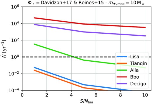
Observable TDE rate with gravitational waves as a function of our ability to detect events from the noise for different gravitational wave detectors. While a detection with LISA and Tianqin is unlikely, the second generation of space-based gravitational wave detectors will observe gravitational waves of TDEs.

Open in new tab Download slide

In order to know what the typical parameters of these possible detections will be, we show in Fig. 11 the distribution functions |$\mathrm{d}^4 \mathcal {P}=\mathrm{d}^4\Gamma /\dot{\Gamma }$| (⁠|$\mathrm{d}^4 \mathcal {P}=\mathrm{d}^4\dot{N}/\dot{N}$|⁠) marginalized on to the different relevant parameters (⁠|$M_\bullet ,\, \beta ,\, m_\star ,\, z$|⁠) for the global (gravitationally observed) population of TDEs.

Figure 11.

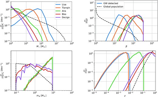
Distribution of TDEs if we were able to detect all of them (‘global population’, dashed lines), and distributions of ‘GW-detected’ TDEs (solid lines) for different gravitational wave detectors (colours).

Open in new tab Download slide

We begin with the global populations of TDEs (black dashed lines in Fig. 11, obtained with Γ), that is the intrinsic distribution of TDEs for our model that may or may not be observed with electromagnetic or gravitational waves.

The distribution with the BH mass (upper left) decreases by |$\sim 2 \mathrm{\, dex}$| in the range |$10^4-10^6\, \mathrm{M}_{\odot }$|⁠, which reflects the fact that both the BH mass function (see Fig. C1) and the TDE rate at fixed BH mass (see Fig. 8) decrease by |$\sim 1 \mathrm{\, dex}$|⁠. The distribution with the penetration factor (upper right) peaks at β ∼ 1, then scales as 1/β² on a wide range of values, and finally smoothly decreases to reach 0 at β = β_max. This is in agreement with previous results (Stone & Metzger 2016; Kochanek 2016a), suggesting a combination of δ-dirac and 1/β² distributions, respectively, in the empty and full loss cone, but we find here an exact continuous distribution, which will be detailed more in depth in Wong, Pfister & Dai 2021. The distribution with the stellar mass (lower left) is similar to that of the underlying stellar mass function chosen, which reflects that stars diffuse similarly as diffusion coefficients are independent of the stellar mass. Finally, the distribution with (the log of) redshift (lower right) scales as z³, which reflects that equation (46) scales as ∂_zΓ ∝ z². In summary, this analysis shows that, albeit inexact, it is reasonable to overall write the global differential rate as:

$$\begin{eqnarray} \frac{\mathrm{d}^4 \Gamma }{\mathrm{d}z\, \mathrm{d}M_\bullet \, \mathrm{d}m_\star \, \mathrm{d}\beta } &\sim& \frac{\Gamma (M_\bullet)}{(1+z)} \times \frac{\beta _{\max } }{\beta ^2 (\beta _{\max } -1)} \times \phi \times \Phi _\bullet\\ && \times \,\, 4\pi c \frac{\chi ^2(z)}{ H(z)} \, . \end{eqnarray}$$

(49)

To our knowledge, this is the first time such a demonstration is obtained, although similar forms of this equation have been used in previous works (e.g. Kochanek 2016b; Toscani et al. 2020). When expressed as this, it clearly appears that if we know the distribution of TDEs, then we have a viable way to probe the BH mass function, the stellar mass function, or even cosmological parameters through the H and χ dependency.

However, we do not have direct access to the distribution of TDEs but to the distribution of gravitationally observed TDEs. This is why we now move the population of TDEs observed with different detectors (solid lines in Fig. 11, obtained with |$\dot{N}$|⁠). We recall that we may not even observe TDEs with LISA or TianQin (S/N_lim = 5 in this case) such that these distributions really makes sense for future-generation detectors. None the less, they can be useful to obtain the most probable events, in the situation in which, by chance, we have a detection with LISA or TianQin.

The distribution with the BH mass (upper left) differs greatly from the one of the intrinsic populations. This reflects that, as discussed in Section 2.1.2, detectors are particularly sensible to BHs for which the Keplerian frequency around the critical radius for direct plunge (κ × r_Sch) is the same as the optimal frequency of the detector : similar to Fig. 3 (right), the peak is at M_{•, opt} (see Table 1). The distribution with the penetration factor (upper right) typically exhibits a peak at β ≳ 20, e.g. β ∼ 20 for LISA and β ∼ 250 for Decigo. This reflects that, for an average population of stars, say with |$\langle m_\star \rangle \sim 1\, \mathrm{M}_{\odot }$|⁠, typically disrupted around BHs with mass |$M_\bullet \sim M_{\bullet ,\, {\rm opt}}$|⁠, detectors are particularly sensible to events with β ∼ β_max [equation (4)]: that is, β ∼ 15 for LISA, and β ∼ 250 for Decigo. The distribution with the stellar mass (lower left) is rather difficult to interpret as, on the one hand, low mass stars are more numerous but, on the other hand, high-mass stars can be detected to higher redshift [equation (12)] and can be disrupted across the entire BH mass range (β_max scales positively with m_⋆). In the end, the distribution for most sensitive detectors, which will be able to detect most TDEs (Bbo and Decigo), is similar to that of the underlying stellar mass function, while the distribution for less-sensitive detectors (LISA, TianQin and Alia) is skewed towards high-mass stars. Finally, the distribution with redshift (lower right), similarly to that of the global rate, scales as z³ at ‘low’ redshift; subsequent evolution is a competition between volume, which makes events more and more numerous, and distance, which makes them less and less detectable; it results in gradual flattening of the distribution where it reaches its maximum (⁠|$z \sim \mathrm{few\, }10^{-3}$| for LISA and |$z \sim \mathrm{few\, }10^{-1}$| for Decigo) and then decreases. This reflects that most detected TDEs will be of stars with a mass |$m_{\star ,\, {\rm opt}}$| (10|$\, \mathrm{M}_{\odot }$|for LISA and 1|$\, \mathrm{M}_{\odot }$|for Decigo) around |$M_{\bullet ,\, {\rm opt}}$| BHs at z_max (Fig. 3) for volume effects, which yields |$\sim \mathrm{few\, }10^{-3}$| for LISA and |$\sim \mathrm{few\, }10^{-1}$| for Decigo.

In summary, we will unlikely detect TDEs with gravitational waves during the LISA and TianQin missions, but next-generation detectors will observe hundreds to tens of thousands of events per year. We also derive a complete β-distribution encompassing, but consistent with, both the full and empty loss cone regimes (black dashed line in the upper right-hand panel of Fig. 11). Finally, we show how the underlying and the observed distributions of TDEs are affected by the different detectors, allowing to predict the properties of the most probable observed events. For LISA, although detections are unlikely, most probable TDE detection will be disruptions of |$\sim 10\, \mathrm{M}_{\odot }$| stars on β ∼ 20 orbits around an |$\sim 5\times 10^5\, \mathrm{M}_{\odot }$| BHs at z ∼ 0.005. For Decigo, most probable TDE detection will be disruptions of |$\sim 1\, \mathrm{M}_{\odot }$| stars on β ∼ 200 orbits around an |$\sim 10^4\, \mathrm{M}_{\odot }$| BHs at z ∼ 0.5. This results in a G magnitude of 15 and 29, or X-ray flux of |$10^{-11}\, \text{erg cm}^{-2}\text{ s}^{-1}$| and |$10^{-16}\, \text{erg cm}^{-2}\text{ s}^{-1}$|⁠, respectively. As a consequence, these TDEs observed with gravitational waves will also be observed by facilities in the electromagnetic spectrum-like Lynx (The Lynx Team 2018), Athena (Nandra et al. 2013), or the LSST (Ivezić et al. 2019). The information encoded in the gravitational wave signal (M_•, β, m_⋆, z but also information on the internal structure of the star, or the spin of the BH, see Stone et al. 2019) combined with those of the electromagnetic signal (which are already used to understand TDEs, e.g. Mockler et al. 2019) will open the multimessenger era for TDEs and unveil new physics currently not well constrained (e.g. Roth et al. 2020b; Bonnerot & Stone 2021; Dai, Lodato & Cheng 2021).

In this section, we focused on the detection rate of several detectors assuming one fiducial model. In the following section, we focus on the case of LISA (in construction detector) and Decigo (next-generation detector) and discuss different models.

4.2 The need for detector improvement

The different models explored in this paper differ by the BH mass function and the maximum stellar mass in the Kroupa stellar mass function (see Section 3.3). We show in Fig. 12 the observable rate of TDEs as a function of |$m_{\star ,\, \max }$|⁠, for the two BH mass functions (colours), for two S/N_lim (line style), and for LISA (left) and Decigo (right).

Figure 12.

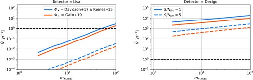
Observable TDE rate with gravitational waves as a function of the maximum stellar mass in the Kroupa stellar mass function. We show the results for LISA (left) and Decigo (right), and in both cases for our two models for the BH mass function (colour, see Section 3.2.1) and ability to detect the signal from the noise (line style).

Open in new tab Download slide

In all cases, we note that there is still a strong dependency with our ability to detect events from the noise.

The case of LISA (left) is interesting because, if we are able to detect events with S/N_lim = 1, there exists a set of models for which there will be up to few detections per year. This means that (non) observations will favour (rule out) these models. To be more precise, if we observe TDEs with LISA, this implies that typical stellar population around BHs is rather young with |$m_{\star ,\, \max } \gtrsim 60 \, \mathrm{M}_{\odot }$|⁠, independently of the BH mass function, and vice versa.

This information can then be used to better interpret the future observations of Decigo (right). Choosing again the example of S/N_lim = 1, if, for instance, ∼10⁴ events are yearly observed, one cannot know if the underlying population is |$\Phi _{\bullet ,\, 1}$| with |$m_{\star ,\, \max }\sim 20\, \mathrm{M}_{\odot }$| or |$\Phi _{\bullet ,\, 2}$| with |$m_{\star ,\, \max }\sim 100\, \mathrm{M}_{\odot }$|⁠, but previous (non) observations with LISA can help in disentangling the two scenarios.

In summary, apart from the optimistic case |$m_{\star ,\, \max }\sim 100\, \mathrm{M}_{\odot }$|⁠, it is quite unlikely that LISA will observe any TDEs during its 4-yr mission. However, (non) observations will already constrain the typical stellar age around BHs and will be useful to better understand future observations.

5 CONCLUSIONS

We determine the rates of possible observations of TDEs with future gravitational wave spacecrafts as well as their possible electromagnetic counterpart. To this purpose, we develop a simple semi-analytical model combining standard gravitational wave and electromagnetic results (Section 2) and rates estimates (Section 3). We summarize our findings below:

LISA could detect gravitational waves from extreme TDEs (⁠|$m_\star \sim 100\, \mathrm{M}_{\odot }$| on an orbit that skims the Schwarzschild radius of a |$10^6\, \mathrm{M}_{\odot }$| BH) up to z_max ∼ 0.1 (see Fig. 3). We provide an analytical expression for z_max [equation (12)].
Under the assumptions that all TDEs produce prompt and luminous optical or X-ray emissions, then all these LISA gravitational detections should be detectable electromagnetically (see Figs 4 and 5).
The TDE rate of a monochromatic stellar population is about 5 times lower than that of a Kroupa stellar population (Fig. 8). Since we remove events for which the star is swallowed whole (assuming a Schwarzschild BH), we find a smooth decay of the TDE rate with M_• starting at |$\sim 10^7\, \mathrm{M}_{\odot }$| BH where |$\sim 0.1\, \mathrm{M}_{\odot }$| stars are being swallowed and finishing at |$\gtrsim 10^8\, \mathrm{M}_{\odot }$| where |$\gt 1\, \mathrm{M}_{\odot }$| stars are being swallowed (see Fig. 6).
This enhancement is in broad agreement with previous analytical results (Fig. 7), although we derive in this paper more detailed rates, in particular, regarding the dependency with the penetration factor β.
The TDE rate overall decreases with the stellar mass and the penetration factor, but its complex variations are depicted in Fig. 9 and will be discussed in more details in Wong et al. 2021.
LISA should not detect any TDEs (Fig. 10), unless BHs are typically embedded by a young stellar population with |$m_{\star ,\, \max }~\gtrsim 60~\, \mathrm{M}_{\odot }$| which, in this situation, could lead up to few 10 events during the duration of the mission (Fig. 12). As such, the number of (non) detections will reveal the typical age surrounding BHs, with (non) detections if BHs are typically embedded in a young (old) stellar population.
The following generation of detectors (Alia, Bbo, and Decigo) will be more sensitive and will be able to yearly detect thousands to millions of events (Fig. 10) at cosmological redshift (Fig. 3), allowing to probe the BH mass function (Fig. 12).
For each detectors and models, we obtain the distribution of parameters (Fig. 11). The most probable BH mass corresponds to BHs for which the Keplerian frequency around the critical radius for direct plunge (κ × r_Sch) is the same as the optimal frequency of the detector (see Table 1). Assuming this most probable BH mass and some typical |$m_\star \sim 1\, \mathrm{M}_{\odot }$|⁠, the most probable penetration factor corresponds to the maximum possible value [equation (4)], and the most probable redshift corresponds to the maximum redshift for the detector [equation (12)].

In order to end up with a finite paper, several assumptions have been made (Kroupa stellar mass function, one single choice of the M_• − σ relation, non-spinning BHs etc.), which may affect the exact rates obtained in this paper. As such, these predictions should be regarded as guidelines. It would be interesting to investigate in depth the detailed effects of other parameters in future studies.

ACKNOWLEDGEMENTS

We thank the anonymous referee carefully reading the first version of the paper and for providing useful comments. HP acknowledges support from the Danish National Research Foundation (DNRF132) and the Hong Kong government (GRF grant HKU27305119, HKU17304821). MT and GL have received funding from the European Union’s Horizon 2020 research and innovation program under the Marie Skłodowska-Curie grant agreement no. 823823 (RISE DUSTBUSTERS project). TW and JLD are supported by the GRF grant from the Hong Kong government under HKU 27305119 and HKU 17304821.

HP’s work would not be possible without the exceptional following python tools: astropy (Astropy Collaboration 2013), ipython (Pérez & Granger 2007), jupyter-notebook (Kluyver et al. 2016), matplotlib (Hunter 2007), numpy (Harris et al. 2020), pandas (pandas development team 2020), scipy (Virtanen et al. 2020), and yt (Turk et al. 2011).

DATA AVAILABILITY

Scripts and data used for this paper are available upon request.

Footnotes

1

See sensitivity curve of different detectors in Fig. A1.

2

In general, P depends on R except for the isochrone potential (Binney & Tremaine 1987). However, its dependency is usually weak and therefore neglected.

3

|$\gamma (z)=\int _0^\infty t^{z-1}e^{-t}\mathrm{d}t$|⁠.

4

|$B(x,a,b)=\int _0^x t^{a-1}(1-t)^{b-1} \mathrm{d}t$|⁠.

5

We report here the correct equation as there is a typo in the original paper, private communications with A. Sesana.

6

We use |$\, \mathrm{cMpc}$| for comoving Mpc.

7

There is actually a small dependency through the Coulomb logarithm factor ln Λ, but this dependency is logarithmic and usually neglected.

REFERENCES

Abbott

B. P.

et al. ,

2017

,

ApJ

,

848

,

L12

10.3847/2041-8213/aa91c9

Crossref

Search ADS

Amaro-Seoane

P.

et al. ,

2017

,

preprint (arXiv:1702.00786)

Astropy Collaboration

2013

,

A&A

,

558

,

A33

10.1051/0004-6361/201322068

Crossref

Search ADS

Baker

J.

et al. ,

2019

,

preprint (arXiv:1907.06482)

Bar-Or

B.

,

Alexander

T.

,

2016

,

ApJ

,

820

,

129

10.3847/0004-637X/820/2/129

Crossref

Search ADS

Barausse

E.

,

Dvorkin

I.

,

Tremmel

M.

,

Volonteri

M.

,

Bonetti

M.

,

2020

,

ApJ

,

904

,

16

10.3847/1538-4357/abba7f

Crossref

Search ADS

Binney

J.

,

Tremaine

S.

,

1987

,

Galactic Dynamics, 1st edn. Princeton Series in Astrophysics

.

Princeton University Press

,

Princeton, NJ

Google Scholar

Google Preview

OpenURL Placeholder Text

WorldCat

Bonnerot

C.

,

Stone

N. C.

,

2021

,

Space Sci. Rev.

,

217

,

16

Chabrier

G.

,

2003

,

PASP

,

115

,

763

10.1086/376392

Crossref

Search ADS

Chen

Y.

,

Yu

Q.

,

Lu

Y.

,

2020

,

ApJ

,

900

,

191

10.3847/1538-4357/aba950

Crossref

Search ADS

Choi

J.

,

Dotter

A.

,

Conroy

C.

,

Cantiello

M.

,

Paxton

B.

,

Johnson

B. D.

,

2016

,

ApJ

,

823

,

102

10.3847/0004-637X/823/2/102

Crossref

Search ADS

Cohn

H.

,

Kulsrud

R. M.

,

1978

,

ApJ

,

226

,

1087

10.1086/156685

Crossref

Search ADS

Colpi

M.

,

Sesana

A.

,

2017

, in

Auger

G.

,

Plagnol

E.

, eds,

An Overview of Gravitational Waves: Theory, Sources and Detection

.

World Scientific Publishing Co. Pte. Ltd

,

Singapore

Google Scholar

Google Preview

OpenURL Placeholder Text

WorldCat

Dai

J. L.

,

Lodato

G.

,

Cheng

R.

,

2021

,

Space Sci. Rev.

,

217

,

12

Dai

L.

,

McKinney

J. C.

,

Roth

N.

,

Ramirez-Ruiz

E.

,

Miller

M. C.

,

2018

,

ApJ

,

859

,

L20

10.3847/2041-8213/aab429

Crossref

Search ADS

Davidzon

I.

et al. ,

2017

,

AAP

,

605

,

A70

Crossref

Search ADS

Evans

C. R.

,

Kochanek

C. S.

,

1989

,

ApJ

,

346

,

L13

10.1086/185567

Crossref

Search ADS

Gallo

E.

,

Sesana

A.

,

2019

,

ApJ

,

883

,

L18

10.3847/2041-8213/ab40c6

Crossref

Search ADS

Goicovic

F. G.

,

Springel

V.

,

Ohlmann

S. T.

,

Pakmor

R.

,

2019

,

MNRAS

,

487

,

981

10.1093/mnras/stz1368

Crossref

Search ADS

Golightly

E. C. A.

,

Coughlin

E. R.

,

Nixon

C. J.

,

2019a

,

ApJ

,

872

,

163

10.3847/1538-4357/aafd2f

Crossref

Search ADS

Golightly

E. C. A.

,

Nixon

C. J.

,

Coughlin

E. R.

,

2019b

,

ApJ

,

882

,

L26

10.3847/2041-8213/ab380d

Crossref

Search ADS

Greene

J. E.

,

Strader

J.

,

Ho

L. C.

,

2019

,

ARA&A

,

58

,

257

Guillochon

J.

,

Ramirez-Ruiz

E.

,

2013

,

ApJ

,

767

,

25

10.1088/0004-637X/767/1/25

Crossref

Search ADS

Guillochon

J.

,

Ramirez-Ruiz

E.

,

Rosswog

S.

,

Kasen

D.

,

2009

,

ApJ

,

705

,

844

10.1088/0004-637X/705/1/844

Crossref

Search ADS

Harris

C. R.

et al. ,

2020

,

Nature

,

585

,

357

10.1038/s41586-020-2649-2

Crossref

Search ADS

PubMed

Harry

G. M.

,

Fritschel

P.

,

Shaddock

D. A.

,

Folkner

W.

,

Phinney

E. S.

,

2006

,

Class. Quantum Gravity

,

23

,

4887

10.1088/0264-9381/23/15/008

Crossref

Search ADS

Hills

J. G.

,

1975

,

Nature

,

254

,

295

10.1038/254295a0

Crossref

Search ADS

Hung

T.

et al. ,

2017

,

ApJ

,

842

,

29

10.3847/1538-4357/aa7337

Crossref

Search ADS

Hunter

J. D.

,

2007

,

Comput. Sci. Eng.

,

9

,

90

Crossref

Search ADS

Ivezić

Ž.

et al. ,

2019

,

ApJ

,

873

,

111

10.3847/1538-4357/ab042c

Crossref

Search ADS

Jones

D. O.

et al. ,

2020

,

ApJ

,

908

,

143

Kesden

M.

,

2012

,

Phys. Rev.

,

85

,

024037

Kippenhahn

R.

,

Weigert

A.

,

1990

,

Stellar Structure and Evolution, XVI

.

Springer-Verlag

,

Berlin Heidelberg

Kluyver

T.

et al. ,

2016

, in

Loizides

F.

,

Schmidt

B.

, eds,

Positioning and Power in Academic Publishing: Players, Agents and Agendas

, p.

87

Kobayashi

S.

,

Laguna

P.

,

Phinney

E. S.

,

Mészáros

P.

,

2004

,

ApJ

,

615

,

855

10.1086/424684

Crossref

Search ADS

Kochanek

C. S.

,

2016a

,

MNRAS

,

458

,

127

10.1093/mnras/stw267

Crossref

Search ADS

Kochanek

C. S.

,

2016b

,

MNRAS

,

461

,

371

10.1093/mnras/stw1290

Crossref

Search ADS

Kormendy

J.

,

Ho

L. C.

,

2013

,

ARAA

,

51

,

511

10.1146/annurev-astro-082708-101811

Crossref

Search ADS

Krolik

J.

,

Piran

T.

,

Ryu

T.

,

2020

,

ApJ

,

904

,

68

10.3847/1538-4357/abc0f6

Crossref

Search ADS

Kroupa

P.

,

2001

,

MNRAS

,

322

,

231

10.1046/j.1365-8711.2001.04022.x

Crossref

Search ADS

Lacy

J. H.

,

Townes

C. H.

,

Hollenbach

D. J.

,

1982

,

ApJ

,

262

,

120

10.1086/160402

Crossref

Search ADS

Lauer

T. R.

et al. ,

2007

,

ApJ

,

664

,

226

10.1086/519229

Crossref

Search ADS

Law-Smith

J. A. P.

,

Coulter

D. A.

,

Guillochon

J.

,

Mockler

B.

,

Ramirez-Ruiz

E.

,

2020

,

ApJ

,

905

,

141

Lightman

A. P.

,

Shapiro

S. L.

,

1977

,

ApJ

,

211

,

244

10.1086/154925

Crossref

Search ADS

Liptai

D.

,

Price

D. J.

,

Mandel

I.

,

Lodato

G.

,

2019

,

preprint (arXiv:1910.10154)

Lodato

G.

,

2012

, in

European Physical Journal Web of Conferences

. p.

01001

Lodato

G.

,

Cheng

R. M.

,

Bonnerot

C.

,

Dai

J. L.

,

2020

,

Space Sci. Rev.

,

216

,

63

Lodato

G.

,

King

A. R.

,

Pringle

J. E.

,

2009

,

MNRAS

,

392

,

332

10.1111/j.1365-2966.2008.14049.x

Crossref

Search ADS

Lodato

G.

,

Rossi

E. M.

,

2011

,

MNRAS

,

410

,

359

10.1111/j.1365-2966.2010.17448.x

Crossref

Search ADS

Luo

J.

et al. ,

2016

,

Class. Quantum Gravity

,

33

,

035010

10.1088/0264-9381/33/3/035010

Crossref

Search ADS

Maggiore

M.

,

2008

,

Gravitational Waves. Vol 1, Theory and Experiments

.

Oxford University Press

,

Oxford

Google Scholar

Google Preview

OpenURL Placeholder Text

WorldCat

Magorrian

J.

,

Tremaine

S.

,

1999

,

MNRAS

,

309

,

447

10.1046/j.1365-8711.1999.02853.x

Crossref

Search ADS

Merloni

A.

et al. ,

2012

,

preprint (arXiv:1209.3114)

Merritt

D.

,

2013

,

Dynamics and Evolution of Galactic Nuclei

.

Princeton University Press

,

Princeton, NJ

Merritt

D.

,

Ferrarese

L.

,

2001

, in

Knapen

J. H.

,

Beckman

J. E.

,

Shlosman

I.

,

Mahoney

T. J.

, eds,

ASP Conf. Ser.

Vol. 249

,

The Central Kiloparsec of Starbursts and AGN: The La Palma Connection

.

Astron. Soc. Pac

,

San Francisco

, p.

335

Google Scholar

Google Preview

OpenURL Placeholder Text

WorldCat

Mockler

B.

,

Guillochon

J.

,

Ramirez-Ruiz

E.

,

2019

,

ApJ

,

872

,

151

10.3847/1538-4357/ab010f

Crossref

Search ADS

Nandra

K.

et al. ,

2013

,

preprint (arXiv:1306.2307)

Pandas Development Team T.

,

2020

,

pandas-dev/pandas: Pandas

,

Available at:

https://pandas.pydata.org/about/citing.html

Pechetti

R.

,

Seth

A.

,

Neumayer

N.

,

Georgiev

I.

,

Kacharov

N.

,

den Brok

M.

,

2019

,

ApJ

,

900

,

32

Pérez

F.

,

Granger

B. E.

,

2007

,

Comput. Sci. Eng.

,

9

,

21

Crossref

Search ADS

Pestoni

B.

,

Bortolas

E.

,

Capelo

P. R.

,

Mayer

L.

,

2021

,

MNRAS

,

500

,

4628

10.1093/mnras/staa3496

Crossref

Search ADS

Pfister

H.

,

Bar-Or

B.

,

Volonteri

M.

,

Dubois

Y.

,

Capelo

P. R.

,

2019b

,

MNRAS

,

488

,

L29

10.1093/mnrasl/slz091

Crossref

Search ADS

Pfister

H.

,

Dai

J.

,

Volonteri

M.

,

Auchettl

K.

,

Trebitsch

M.

,

Ramirez-Ruiz

E.

,

2020b

,

MNRAS

,

500

,

3944

Pfister

H.

,

Lupi

A.

,

Capelo

P. R.

,

Volonteri

M.

,

Bellovary

J. M.

,

Dotti

M.

,

2017

,

MNRAS

,

471

,

3646

10.1093/mnras/stx1853

Crossref

Search ADS

Pfister

H.

,

Volonteri

M.

,

Dubois

Y.

,

Dotti

M.

,

Colpi

M.

,

2019a

,

MNRAS

,

486

,

101

10.1093/mnras/stz822

Crossref

Search ADS

Pfister

H.

,

Volonteri

M.

,

Lixin Dai

J.

,

Colpi

M.

,

2020a

,

MNRAS

,

497

,

2276

Piran

T.

,

Svirski

G.

,

Krolik

J.

,

Cheng

R. M.

,

Shiokawa

H.

,

2015

,

ApJ

,

806

,

164

10.1088/0004-637X/806/2/164

Crossref

Search ADS

Planck Collaboration XIII

,

2016

,

AAP

,

594

,

A13

Crossref

Search ADS

Rees

M. J.

,

1988

,

Nature

,

333

,

523

10.1038/333523a0

Crossref

Search ADS

Reines

A. E.

,

Volonteri

M.

,

2015

,

ApJ

,

813

,

82

10.1088/0004-637X/813/2/82

Crossref

Search ADS

Roth

N.

,

Kasen

D.

,

2018

,

ApJ

,

855

,

54

10.3847/1538-4357/aaaec6

Crossref

Search ADS

Roth

N.

,

Rossi

E. M.

,

Krolik

J.

,

Piran

T.

,

Mockler

B.

,

Kasen

D.

,

2020b

,

Space Sci. Rev.

,

216

,

114

Roth

N.

,

van Velzen

S.

,

Cenko

S. B.

,

Mushotzky

R. F.

,

2020a

,

ApJ

,

910

,

93

Ryu

T.

,

Krolik

J.

,

Piran

T.

,

2020a

,

ApJ

,

904

,

73

10.3847/1538-4357/abbf4d

Crossref

Search ADS

Ryu

T.

,

Krolik

J.

,

Piran

T.

,

Noble

S. C.

,

2020b

,

ApJ

,

904

,

98

10.3847/1538-4357/abb3cf

Crossref

Search ADS

Ryu

T.

,

Krolik

J.

,

Piran

T.

,

Noble

S. C.

,

2020c

,

ApJ

,

904

,

99

10.3847/1538-4357/abb3cd

Crossref

Search ADS

Ryu

T.

,

Krolik

J.

,

Piran

T.

,

Noble

S. C.

,

2020d

,

ApJ

,

904

,

100

10.3847/1538-4357/abb3ce

Crossref

Search ADS

Sacchi

A.

,

Lodato

G.

,

2019

,

MNRAS

,

486

,

1833

10.1093/mnras/stz981

Crossref

Search ADS

Salpeter

E. E.

,

1955

,

ApJ

,

121

,

161

10.1086/145971

Crossref

Search ADS

Sánchez-Janssen

R.

et al. ,

2019

,

ApJ

,

878

,

18

10.3847/1538-4357/aaf4fd

Crossref

Search ADS

Sato

S.

et al. ,

2009

,

J. Phys. Conf. Ser.

,

154

,

012040

Saxton

R.

,

Komossa

S.

,

Auchettl

K.

,

Jonker

P. G.

,

2020

,

Space Sci. Rev.

,

216

,

85

Shiokawa

H.

,

Krolik

J. H.

,

Cheng

R. M.

,

Piran

T.

,

Noble

S. C.

,

2015

,

ApJ

,

804

,

85

10.1088/0004-637X/804/2/85

Crossref

Search ADS

Spitzer Lyman

J.

,

Hart

M. H.

,

1971

,

ApJ

,

164

,

399

10.1086/150855

Crossref

Search ADS

Stone

N. C.

,

Kesden

M.

,

Cheng

R. M.

,

van Velzen

S.

,

2019

,

Gen. Relativ. Gravit.

,

51

,

30

10.1007/s10714-019-2510-9

Crossref

Search ADS

Stone

N. C.

,

Metzger

B. D.

,

2016

,

MNRAS

,

455

,

859

10.1093/mnras/stv2281

Crossref

Search ADS

Stone

N. C.

,

Vasiliev

E.

,

Kesden

M.

,

Rossi

E. M.

,

Perets

H. B.

,

Amaro-Seoane

P.

,

2020

,

Space Sci. Rev.

,

216

,

35

10.1007/s11214-020-00651-4

Crossref

Search ADS

Stone

N.

,

Sari

R.

,

Loeb

A.

,

2013

,

MNRAS

,

435

,

1809

10.1093/mnras/stt1270

Crossref

Search ADS

Strubbe

L. E.

,

2011

,

PhD thesis

,

University of California

,

Berkeley

The Lynx Team

,

2018

,

preprint (arXiv:1809.09642)

Toscani

M.

,

Lodato

G.

,

Nealon

R.

,

2019

,

MNRAS

,

489

,

699

10.1093/mnras/stz2201

Crossref

Search ADS

Toscani

M.

,

Rossi

E. M.

,

Lodato

G.

,

2020

,

MNRAS

,

498

,

507

10.1093/mnras/staa2290

Crossref

Search ADS

Tremmel

M.

,

Governato

F.

,

Volonteri

M.

,

Quinn

T. R.

,

2015

,

MNRAS

,

451

,

1868

10.1093/mnras/stv1060

Crossref

Search ADS

Turk

M. J.

,

Smith

B. D.

,

Oishi

J. S.

,

Skory

S.

,

Skillman

S. W.

,

Abel

T.

,

Norman

M. L.

,

2011

,

ApJS

,

192

,

9

10.1088/0067-0049/192/1/9

Crossref

Search ADS

Ulmer

A.

,

1999

,

ApJ

,

514

,

180

10.1086/306909

Crossref

Search ADS

van Velzen

S.

et al. ,

2016

,

Science

,

351

,

62

10.1126/science.aad1182

Crossref

Search ADS

PubMed

van Velzen

S.

et al. ,

2020a

,

Science

,

351

,

62

van Velzen

S.

,

2018

,

ApJ

,

852

,

72

10.3847/1538-4357/aa998e

Crossref

Search ADS

van Velzen

S.

,

Holoien

T. W. S.

,

Onori

F.

,

Hung

T.

,

Arcavi

I.

,

2020b

,

Space Sci. Rev.

,

216

,

124

Vasiliev

E.

,

2017

,

ApJ

,

848

,

10

10.3847/1538-4357/aa8cc8

Crossref

Search ADS

Virtanen

P.

et al. ,

2020

,

Nature Methods

,

17

,

261

Crossref

Search ADS

PubMed

Volonteri

M.

,

Haardt

F.

,

Madau

P.

,

2003

,

ApJ

,

582

,

559

10.1086/344675

Crossref

Search ADS

Wang

J.

,

Merritt

D.

,

2004

,

ApJ

,

600

,

149

10.1086/379767

Crossref

Search ADS

Wevers

T.

,

van Velzen

S.

,

Jonker

P. G.

,

Stone

N. C.

,

Hung

T.

,

Onori

F.

,

Gezari

S.

,

Blagorodnova

N.

,

2017

,

MNRAS

,

471

,

1694

10.1093/mnras/stx1703

Crossref

Search ADS

Wong

T. H. T.

,

Pfister

H.

,

Dai

L.

,

2021

,

preprint (arXiv:2111.09173)

APPENDIX A: SENSITIVITY OF GRAVITATIONAL WAVES DETECTOR

We download the sensitivity curves of several instruments on http://gwplotter.com/http://gwplotter.com/ and report them in Fig. A1. While we use the numerical value for this work, it can be useful to have a simple analytical expression to understand the results. Using a simple χ-square regression in the log–log plane, we fit each curves with the following functional:

$$\begin{eqnarray} h_\mathrm{det}(f) = h_\mathrm{opt} \left(\frac{f}{f_\mathrm{opt}} \right)^{-a} \left(\left(\frac{f}{f_\mathrm{opt}} \right)^{c} +1 \right)^{\frac{b + a}{c}} \, , \end{eqnarray}$$

(A1)

where f_opt and h_opt are, respectively, the optimal frequency and strain of the detector, and a and b are the logarithmic slopes for f ≪ f_opt and f ≫ f_opt. The fitting parameters can be found in Table A1 with the resulting curve shown with dashed black lines in Fig. A1.

Figure A1.

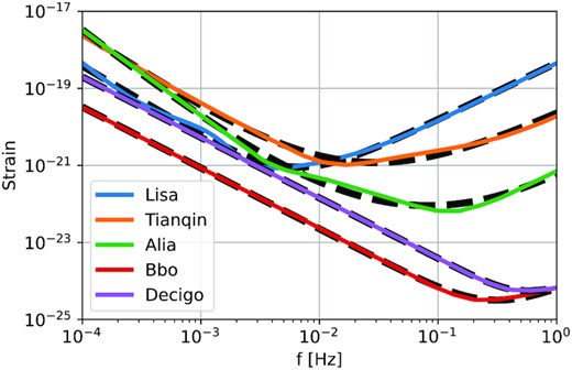
Sensitivity curve as a function of frequency for several gravitational wave detectors (colours) as well as the fit (black dashed lines) with equation (A1).

Open in new tab Download slide

Table A1.

Open in new tab

Best-fitting parameters of the strain of the different detectors with equation (A1).

Detector	f_opt	h_opt	a	b	c
	Hz	10⁻²¹
LISA	6 × 10⁻³	0.2	1.8	1.5	1.7
Tianqin	0.02	7	2.0	1.4	0.8
Alia	0.08	0.02	2.5	2.3	0.6
Bbo	0.3	0.01	1.6	1.2	2.0
Decigo	0.4	0.04	1.6	0.7	3.3

Detector	f_opt	h_opt	a	b	c
	Hz	10⁻²¹
LISA	6 × 10⁻³	0.2	1.8	1.5	1.7
Tianqin	0.02	7	2.0	1.4	0.8
Alia	0.08	0.02	2.5	2.3	0.6
Bbo	0.3	0.01	1.6	1.2	2.0
Decigo	0.4	0.04	1.6	0.7	3.3

Table A1.

Open in new tab

Best-fitting parameters of the strain of the different detectors with equation (A1).

Detector	f_opt	h_opt	a	b	c
	Hz	10⁻²¹
LISA	6 × 10⁻³	0.2	1.8	1.5	1.7
Tianqin	0.02	7	2.0	1.4	0.8
Alia	0.08	0.02	2.5	2.3	0.6
Bbo	0.3	0.01	1.6	1.2	2.0
Decigo	0.4	0.04	1.6	0.7	3.3

Detector	f_opt	h_opt	a	b	c
	Hz	10⁻²¹
LISA	6 × 10⁻³	0.2	1.8	1.5	1.7
Tianqin	0.02	7	2.0	1.4	0.8
Alia	0.08	0.02	2.5	2.3	0.6
Bbo	0.3	0.01	1.6	1.2	2.0
Decigo	0.4	0.04	1.6	0.7	3.3

APPENDIX B: FOKKER–PLANCK EQUATION WITH A STELLAR POPULATION

In this appendix, we show how we can use the formalism developed for monochromatic stellar population to study a more complex population of stars. It is mostly a summary and combination of the works of Magorrian & Tremaine (1999) and Strubbe (2011).

B1 Diffusion coefficients

If the medium is homogeneous such that the stellar mass function (ϕ) is independent of position and time, then we may write the density function f_⋆ as:

$$\begin{eqnarray} f_\star ({\bf r},{\bf v},m_\star) \mathrm{d}{\bf r} \mathrm{d}{\bf v} \mathrm{d}m_\star = f({\bf r},{\bf v})\mathrm{d}{\bf r} \mathrm{d}{\bf v} \times \phi (m_\star) \mathrm{d}m_\star \, . \end{eqnarray}$$

(B1)

Following Section 8.3 from Binney & Tremaine (1987), assuming the background follow the density f(r, v), we define ψ(w, Δw, m_⋆, m_scat)d⁶Δwdt as the probability that a star of mass m_⋆ is scattered from w to w + Δw (w = (r, v)) by a background star of mass m_scat during a transition time dt. Since the background is made of a population of star with distribution ϕ, the probability that a star of mass m_⋆ is scattered from w to w + Δw (w = (r, v)) by the background during dt is:

$$\begin{eqnarray} &&{\psi _\star ({\bf w},\Delta {\bf w}, m_\star) \mathrm{d}^6 \Delta {\bf w} \mathrm{d}t }\\ &&{\quad= \mathrm{d}^6 \Delta {\bf w} \mathrm{d}t \int \phi (m_\mathrm{scat}) \psi ({\bf w},\Delta {\bf w}, m_\star , m_\mathrm{scat}) \mathrm{d}m_\mathrm{scat} \, .} \end{eqnarray}$$

(B2)

This allows to classically write the evolution of f_⋆ as a Fokker–Planck equation:

$$\begin{eqnarray} \frac{\mathrm{d}f_\star }{\mathrm{d}t} &=& - \sum _{i=1}^3\frac{\partial }{\partial v_i}\left[f_\star ({\bf w}, m_\star) D_\star (\Delta v_i, m_\star) \right] \\ &&+ \,\, \frac{1}{2} \sum _{i,j=1}^3\frac{\partial ^2}{\partial v_i\partial v_j}\left[f_\star ({\bf w}, m_\star) D_\star (\Delta v_i \Delta v_j, m_\star) \right] \, , \end{eqnarray}$$

(B3)

where we have defined the diffusion coefficient which, a priori, depends on m_⋆:

$$\begin{eqnarray} D_\star (\Delta v_i ,m_\star) &=& \int \Delta v_i \psi _\star ({\bf w},\Delta {\bf w}, m_\star) \mathrm{d}^6\Delta {\bf w} \end{eqnarray}$$

(B4)

$$\begin{eqnarray} &=& \int \phi (m_\mathrm{scat}) \mathrm{d}m_\mathrm{scat} \\ &&\times \left [ \int \Delta v_i \psi ({\bf w},\Delta {\bf w}, m_\star , m_\mathrm{scat}) \mathrm{d}^6\Delta {\bf w}\, \right ] \end{eqnarray}$$

(B5)

$$\begin{eqnarray} = \int \phi (m_\mathrm{scat}) D(\Delta v_i, m_\star , m_\mathrm{scat}) \mathrm{d}m_\mathrm{scat} \, , \end{eqnarray}$$

(B6)

and D(Δv_i, m_⋆, m_scat) is the diffusion coefficient of test particle of mass m_⋆ moving in a monochromatic population of star m_scat with density function f(r, v) (see §8.3 from Binney & Tremaine 1987).

When written as this, equation (B3) shows that the evolution of a star with mass m_{⋆, 1} differs from the evolution of a star with mass m_{⋆, 2} because their diffusion coefficients differ. This means that to study the evolution of our system, one should study a set of coupled equations, with one Fokker–Planck equation for each mass.

B2 The particular case of TDEs

This set of coupled Fokker–Planck equations can be greatly simplified in the case of TDEs. After changing variables from w to (minus the specific) energy (E = −v²/2 + Ψ(r), Ψ is the potential) and |$R=J^2/J^2_c(E)$| (J = |r∧v| is the angular momentum and J_c(E) is the circular angular momentum at a given energy), a Fokker–Planck equation for f_⋆ can still be written. Neglecting diffusion in E as it relaxes on a longer time-scale than R (Lightman & Shapiro 1977; Cohn & Kulsrud 1978; Merritt 2013), this yields:

$$\begin{eqnarray} \frac{\mathrm{d}f_\star }{\mathrm{d}t} &=& \frac{\partial }{\partial R}\Bigl [ -f_\star D_\star (\Delta R, m_\star) \end{eqnarray}$$

(B7)

$$\begin{eqnarray} +\,\,\frac{1}{2} \frac{\partial }{\partial R} [f_\star D_\star ((\Delta R)^2, m_\star)] \Bigr ] \, . \end{eqnarray}$$

(B8)

Here again, D_⋆(., m_⋆) are the diffusion coefficients and a priori depend in m_⋆.

The diffusion coefficient of interest can be computed (Lightman & Shapiro 1977; Magorrian & Tremaine 1999; Bar-Or & Alexander 2016; Stone & Metzger 2016):

$$\begin{eqnarray} D_\star (\Delta R, m_\star) &=& \frac{r^2 D_\star ((\Delta v_\perp)^2, m_\star)}{J^2_c} \end{eqnarray}$$

(B9)

$$\begin{eqnarray} D_\star ((\Delta R)^2, m_\star) &=& 2RD_\star (\Delta R, m_\star)\, , \end{eqnarray}$$

(B10)

where D_⋆((Δv_⊥)², m_⋆) is the diffusion coefficient in (Δv_⊥)², corresponding to the orthogonal component of the variation of the velocity. Using equation (B6) and that D((Δv_⊥)², m_⋆, m_scat) is [equation (8 A-22) of Binney & Tremaine 1987]:

$$\begin{eqnarray} D((\Delta v_\perp)^2, m_\star , m_\mathrm{scat}) &=& \frac{32 \pi ^2 \, \mathrm{G}^2 m^2_\mathrm{scat} \ln \Lambda }{3 v}\ \\ &&\times \,\Biggr(\int _0^v \Biggr(3 \tilde{v}^2 - \frac{\tilde{v}^4}{v^2}\Biggr) f({\bf r}, \tilde{v}) \mathrm{d}\tilde{v}\\ &&+\,\, 2v \int _v^\infty \tilde{v} f({\bf r}, \tilde{v}) \mathrm{d}\tilde{v} \Biggr) \, , \end{eqnarray}$$

(B11)

we have the remarkable result that D_⋆((Δv_⊥)², m_⋆), hence D_⋆(ΔR, m_⋆) and D_⋆((ΔR)², m_⋆), which are the two diffusion coefficients of interest for us, are independent⁷ of m_⋆. This means that, under our assumptions, the evolution of a test particle is independent of its mass, and everything happens as if the particle was moving in a background composed by stars of mass |$\langle m^2_\star \rangle ^{1/2}=\left(\int m^2_{\rm scat}\phi (m_{\rm scat})\mathrm{d}m_{\rm scat}\right)^{1/2}$|⁠, that is |$D_\star (\Delta R)=D(\Delta R, m_\mathrm{scat}=\langle m^2_\star \rangle ^{1/2})=\mu$| (note that we have now dropped the m_⋆ dependency).

All this allows to write a Fokker–Planck equation for f:

$$\begin{eqnarray} \frac{\mathrm{d}f}{\mathrm{d}t} &=& \frac{\partial }{\partial R}\Bigl [ -f D_\star (\Delta R) \end{eqnarray}$$

(B12)

$$\begin{eqnarray} +\frac{1}{2} \frac{\partial }{\partial R} [f D_\star ((\Delta R)^2)] \Bigr ] \end{eqnarray}$$

(B13)

$$\begin{eqnarray} = \mu \frac{\partial }{\partial R}\left(R \frac{\partial f}{\partial R} \right)\, , \end{eqnarray}$$

(B14)

where we recognize the starting point of estimates of TDE rates (e.g. Merritt 2013).

In conclusion, for our purpose and under approximation, the evolution of a test mass in a medium composed by a stellar population is the same as a test mass in a medium composed single type of stars with mass |$\langle m^2_\star \rangle ^{1/2}$|⁠.

APPENDIX C: BH MASS FUNCTION

We report in Fig. C1 the two BH mass functions used in this work. This simple plot emphasizes our current poor knowledge about BH population, even at low redshift.

Figure C1.

The BH mass functions used in this work: Φ_{•, 1}, which results from the combination of Davidzon et al. (2017) and Reines & Volonteri (2015), is shown at two different redshifts, and Φ_{•, 2} which is directly taken from Gallo & Sesana (2019).

Open in new tab Download slide

Author notes

Sophie and Tycho Brahe Fellow.

This article is published and distributed under the terms of the Oxford University Press, Standard Journals Publication Model (https://dbpia.nl.go.kr/journals/pages/open_access/funder_policies/chorus/standard_publication_model)

Download all slides

Month:	Total Views:
January 2022	40
February 2022	15
March 2022	22
April 2022	18
May 2022	3
June 2022	3
July 2022	12
August 2022	6
September 2022	16
October 2022	12
November 2022	8
December 2022	6
January 2023	8
February 2023	10
March 2023	3
April 2023	6
May 2023	17
June 2023	2
July 2023	2
September 2023	7
October 2023	16
November 2023	1
December 2023	3
January 2024	9
February 2024	30
March 2024	21
April 2024	12
May 2024	19
June 2024	16
July 2024	23
August 2024	22
September 2024	19
October 2024	22
November 2024	19
December 2024	22
January 2025	14
February 2025	21
March 2025	18
April 2025	10
May 2025	5

Article Contents

Observable gravitational waves from tidal disruption events and their electromagnetic counterpart

ABSTRACT

1 INTRODUCTION

2 DETECTION OF SINGLE EVENTS

2.1 Gravitational waves

2.1.1 Formalism

2.1.2 Maximum redshift for detection

2.2 Electromagnetic counterpart

2.2.1 Optical emission

2.2.2 X-ray emission

3 TDE RATES

3.1 Single galaxy

3.1.1 Loss cone dynamics

3.1.2 Stellar properties around the BH

3.1.3 Summary

3.2 Population of galaxies

3.2.1 BH mass function

3.2.2 Summary

3.3 Caveats

4 TOTAL RATES OF GRAVITATIONALLY OBSERVED TDES

4.1 Typical numbers of observations and distributions

4.2 The need for detector improvement

5 CONCLUSIONS

ACKNOWLEDGEMENTS

DATA AVAILABILITY

Footnotes

REFERENCES

APPENDIX A: SENSITIVITY OF GRAVITATIONAL WAVES DETECTOR

APPENDIX B: FOKKER–PLANCK EQUATION WITH A STELLAR POPULATION

B1 Diffusion coefficients

B2 The particular case of TDEs

APPENDIX C: BH MASS FUNCTION

Author notes

Citations

Views

Altmetric

Email alerts

Astrophysics Data System

Citing articles via

Latest

Most Read

Most Cited

This Feature Is Available To Subscribers Only