


ABSTRACT
X-ray emission from the gravitational wave transient GW170817 is well described as non-thermal afterglow radiation produced by a structured relativistic jet viewed off-axis. We show that the X-ray counterpart continues to be detected at 3.3 years after the merger. Such long-lasting signal is not a prediction of the earlier jet models characterized by a narrow jet core and a viewing angle ≈20 deg, and is spurring a renewed interest in the origin of the X-ray emission. We present a comprehensive analysis of the X-ray dataset aimed at clarifying existing discrepancies in the literature, and in particular the presence of an X-ray rebrightening at late times. Our analysis does not find evidence for an increase in the X-ray flux, but confirms a growing tension between the observations and the jet model. Further observations at radio and X-ray wavelengths would be critical to break the degeneracy between models.
1 INTRODUCTION
The ground-breaking discovery of the binary neutron star (BNS) merger GW170817 by the LIGO/VIRGO Collaboration (Abbott et al. 2017a) and the near-coincident detection, with a delay of 1.7 s, of the short duration gamma-ray burst GRB 170718A (Abbott et al. 2017b) heralded a new era of multi-messenger astrophysics combining gravitational waves (GW) with photons. GRB 170817A, at a distance of only ∼ 40 Mpc, is the least luminous short GRB known to date. It does not display the standard fading afterglow of GRBs, but a delayed X-ray (Troja et al. 2017) and radio (Hallinan et al. 2017) emission. Its broadband afterglow is seen to rise as Fν ∝ t0.8 (Troja et al. 2018; Lyman et al. 2018; Margutti et al. 2018; Ruan et al. 2018), peak at ∼ 160 d after the merger (Dobie et al. 2018; D’Avanzo et al. 2018; Piro et al. 2019), and then rapidly decay as Fν ∝ t−2.2 (Mooley et al. 2018; Lamb et al. 2019; Troja et al. 2019).
The afterglow behaviour is now commonly interpreted as emission from a structured GRB jet viewed off-axis, with viewing angle θv ≈ 20-30 deg (Troja et al. 2017; Lazzati et al. 2018; Lyman et al. 2018; D’Avanzo et al. 2018; Xie, Zrake & MacFadyen 2018; Margutti et al. 2018; Resmi et al. 2018; Mooley et al. 2018; Ghirlanda et al. 2019; Lamb et al. 2019; Ryan et al. 2020; Troja et al. 2019; Beniamini, Granot & Gill 2020; Nathanail et al. 2020; Troja et al. 2020; Makhathini et al. 2020). The close distance of the event and its bright long-lived emission allowed for an unprecedented insight into the structure of GRB jets and novel constraints on the Hubble Constant (Hotokezaka et al. 2019; Nakar & Piran 2021). Continued monitoring of the GW afterglow will further deepen our understanding of GRB physics into a poorly explored regime. Whereas the rising slope of the light curve is dictated by the initial jet structure and the viewing angle (Ryan et al. 2020; Takahashi & Ioka 2020, 2021), its late-time evolution (postpeak) will be dictated by the spreading dynamics of the jet and its deceleration into a non-relativistic flow. Although the measured decay slope is sufficiently steep to confirm the presence of a collimated jet (Troja et al. 2018), the exact predicted slope at this stage remains sensitive to details in the modeling and to the detailed features of the actual outflow. Other factors can impact the slope as well (Troja et al. 2020), such as a change in the properties of particle-shock acceleration across the transition from relativistic to non-relativistic shocks.
Most interestingly, now that the emission from the relativistic jet is fading away, new emission components may become visible (Troja et al. 2020; Balasubramanian et al. 2021; Hajela et al. 2021). A popular model is the so called ‘radio flare’ - non-thermal radiation produced by the deceleration of the fastest merger ejecta (Nakar & Piran 2011; Hotokezaka et al. 2018), also referred to as kilonova afterglow (Kathirgamaraju, Barniol Duran & Giannios 2018). This new component would appear as a slowly rising radio counterpart, visible a few year after the merger, although interaction between the relativistic jet and the merger ejecta may quench it and further delay its onset (Margalit & Piran 2020; Ricci et al. 2021). Depending on the spectral shape of the radio flare, its signal may also be detectable at X-ray energies (Kathirgamaraju et al. 2018; Hajela et al. 2019; Troja et al. 2020). Late-time emission from the central compact object was also discussed (Murase et al. 2018; Piro et al. 2019), and could unveil the nature of the elusive merger remnant.
Any deviation from the relativistic structured jet model is of great interest, whether it belongs to the jet dynamical evolution, the changing nature of particle acceleration once shocks enter the trans-relativistic regime, or to the emergence of an additional components. However, its identification is complicated by the faintness of the source which, at this point in time, is only marginally detectable with the existing instrumentation. Different statistical treatments of the low-count regime and/or different modeling of the instrumental effects might introduce a systematic uncertainty in the flux measurements. This issue seems to be particularly relevant for the X-ray fluxes reported in the literature with values differing by up to a factor of two for the same dataset.
In this work, we present a homogeneous re-analysis of the X-ray dataset aimed at characterizing such differences and, in particular, at addressing the onset of a new component of emission at ≈3 yr post-merger, as discussed in Troja et al. (2020) and recently more firmly claimed by Hajela et al. (2021). In Section 2, we present the observations and data analysis. In Section 3, we discuss a comparison of the jet model to these latest observations, and in Section 4 we summarize our findings. Throughout this paper, times are referenced to the GRB trigger. We adopt a standard ΛCDM cosmology (Planck Collaboration et al. 2018). Unless otherwise stated, the quoted errors are at the 68 per cent confidence level, and upper limits are at the 3 σ confidence level.
2 OBSERVATIONS AND DATA ANALYSIS
The target has been regularly monitored with the Chandra X-ray Telescope starting on August 19, 2017 (T0 + 2.3 d) until January 27, 2021 (T0 + 1258.7 d). The entire dataset, consisting of 31 observations spread over 11 epochs, was reprocessed using the latest release of the Chandra Interactive Analysis of Observations (CIAO v. 4.13; Fruscione et al. 2006) and calibration files (CALDB 4.9.4).
We follow the same steps described in Troja et al. (2020), including background filtering and astrometric alignment of each observation. Aperture photometry was performed in the broad 0.5- 7.0 keV energy band. Since the target is placed close to the optical axis, the point spread function (PSF) can be considered symmetric and source counts are extracted using a circular aperture with radius of 1.5″. If less than 15 counts are extracted, we use a smaller radius of 1.0″ in order to optimize the signal to noise ratio. Aperture corrections are derived through the task arfcorr and are typically ≲1.1. The background level is estimated from two nearby source-free circular regions with radius ≳15″.
The final net count rate is then derived as |$r_s = \eta \, (N - B \times A_s / A_b) \Delta t^{-1}$|, where N and B are the measured total and background counts within the extraction regions of area As and Ab, respectively; η is the energy-dependent aperture correction, and Δt the exposure time of each observation. The detection significance and confidence intervals on the count rates are calculated following Kraft, Burrows & Nousek (1991). Except for the first observation at 2.3 d (ObsID 18955), X-ray emission from the position of GW170817 is detected at all epochs with significance ≳3 σ. A comparison between our results and the values reported in the literature (Hajela et al. 2021; Makhathini et al. 2020; Hajela et al. 2020, 2019; Nynka et al. 2018) shows an overall consistency of the derived count rates (Fig. 1). The values of Hajela et al. (2021) and Makhathini et al. (2020) (priv. comm.) appear systematically lower by a factor ≈1.1, a value consistent with the aperture correction applied in this work. A discrepancy worth of note is the upper limit at 2.3 d. Within our source extraction region, we measure zero counts in a 24.6 ks exposure, from which we derive a 3 σ upper limit of 2.5 × 10⁻⁴ cts s−1, twice the value reported in other works (Hajela et al. 2021, 2019; Nynka et al. 2018) and five times higher than the value quoted in Makhathini et al. (2020). Since we already measure the minimum number of counts, we attribute this difference to the statistical treatment of upper limits. Our limit is derived using the formulation of Kraft et al. (1991), and a similar value is obtained using the approximations of Gehrels (1986). Our results are listed in Table 1 for each epoch, whereas the detailed analysis of each observation is reported in the Appendix (see Table 2).
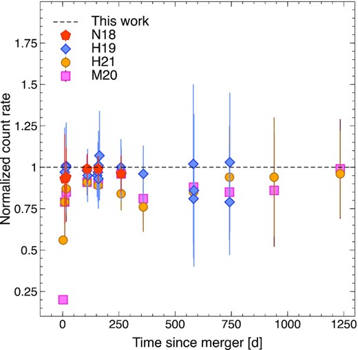
Count-rates presented in the literature (Nynka et al. 2018; Hajela et al. 2019, 2020; Makhathini et al. 2020; Hajela et al. 2021) normalized by the values derived in this work. This comparison shows an overall agreement of the different analyses, except for the first data point at 2.3 d. Other differences may depend on the aperture correction and whether the reported count-rates include it or not.
Chandra X-ray observations of GW170817.
| Γ = 1.585 | Γ free | |||||||
|---|---|---|---|---|---|---|---|---|
| Epoch | T-T0 | Exposure | Count ratea | ECFb | Fluxc,d | ECFb | Fluxc | ObsID |
| (d) | (ks) | [0.5-7.0 keV] | [0.3-10 keV] | [0.3-10 keV] | ||||
| 1 | 2.33 | 24.6 | <2.5 | 1.65 | <4.1 | – | – | 18955 |
| 2 | 9.2 | 49.4 | 2.9|$^{+0.9}_{-0.7}$| | 1.65 | 4.7|$^{+1.5}_{-1.2}$| | 1.92|$^{+0.8}_{-0.3}$| | 5.8|$^{+2}_{-1.4}$| | 19294 |
| 3 | 15.7 | 93.4 | 3.4|$^{+0.7}_{-0.7}$| | 1.65 | 5.6|$^{+1.2}_{-1.2}$| | 1.56|$^{+0.19}_{-0.10}$| | 5.3|$^{+1.2}_{-1.1}$| | 20728, 18988 |
| 4 | 108.7 | 98.8 | 14.9|$^{+1.2}_{-1.2}$| | 1.67 | 25|$^{+2}_{-2}$| | 1.66|$^{+0.11}_{-0.06}$| | 25|$^{+3}_{-2}$| | 20860, 20861 |
| 5 | 158 | 104.9 | 15.4|$^{+1.2}_{-1.2}$| | 1.69 | 26|$^{+2}_{-2}$| | 1.61|$^{+0.06}_{-0.02}$| | 25|$^{+2}_{-2}$| | 20936, 20938, 20937, |
| 20939, 20945 | ||||||||
| 6 | 260.0 | 96.8 | 8.2|$^{+0.9}_{-0.9}$| | 1.71 | 14.0|$^{+1.7}_{-1.7}$| | 1.66|$^{+0.14}_{-0.04}$| | 13.6|$^{+1.9}_{-1.6}$| | 21080, 21090 |
| 7 | 358.6 | 67.2 | 5.2|$^{+1.0}_{-0.9}$| | 1.73 | 9.0|$^{+1.7}_{-1.5}$| | 1.78|$^{+0.3}_{-0.11}$| | 9.3|$^{+2}_{-1.7}$| | 21371 |
| 8 | 582.0 | 98.3 | 1.7|$^{+0.4}_{-0.5}$| | 1.80 | 3.1|$^{+0.7}_{-0.9}$| | 1.97|$^{+0.18}_{-0.2}$| | 3.4|$^{+1.0}_{-1.0}$| | 21322, 22157, 22158 |
| 9 | 741.7 | 98.9 | 1.1|$^{+0.3}_{-0.4}$| | 1.85 | 2.0|$^{+0.5}_{-0.7}$| | 2.90|$^{+1.00}_{-0.6}$| | 3.1|$^{+1.6}_{-1.3}$| | 21372, 22736, 22737 |
| 10 | 940 | 96.6 | 0.8|$^{+0.3}_{-0.3}$| | 1.91 | 1.6|$^{+0.5}_{-0.7}$| | 2.00|$^{+0.6}_{-0.2}$| | 1.6|$^{+0.9}_{-0.7}$| | 21323, 23183, 23184 |
| 23185 | ||||||||
| 11a | 1212 | 91.1 | 1.2|$^{+0.4}_{-0.3}$| | 2.00 | 2.3|$^{+0.9}_{-0.6}$| | 2.30|$^{+1.2}_{-0.3}$| | 2.7|$^{+1.5}_{-0.8}$| | 22677, 24887, 24888 |
| 24889 | ||||||||
| 11b | 1255 | 97.9 | 0.5|$^{+0.2}_{-0.2}$| | 1.99 | 1.0|$^{+0.5}_{-0.5}$| | 2.30|$^{+1.2}_{-0.3}$| | 1.1|$^{+0.8}_{-0.6}$| | 23870, 24923, 24924 |
| 22677, 24887, 24888, | ||||||||
| 11 | 1234 | 189 | 0.8|$^{+0.2}_{-0.2}$| | 2.00 | 1.6|$^{+0.5}_{-0.5}$| | 2.30|$^{+1.2}_{-0.3}$| | 1.8|$^{+1.1}_{-0.6}$| | 24889, 23870, 24923, |
| 24924 | ||||||||
Notes.a Count rates are in units of 10−4 cts s−1. All the values are corrected for PSF losses.
b ECFs are in units of 10−11 er g cm−2 ct−1
c Fluxes in units of 10−15 erg cm −2 s−1. Values are corrected for Galactic extinction.
d The quoted values can be converted into flux densities (in units of Jy) by multiplying them by a factor of 86027 (1 keV), or 33553 (5 keV). We adopt a conversion to X-ray luminosity of (2.0 ± 0.2) × 1053 cm2.
We then convert the observed count-rates into X-ray fluxes by folding the afterglow spectral shape with the instrumental response. A joint spectral fit of the radio, optical, and X-ray data shows a power-law spectrum with photon index Γ = 1.585 ± 0.005 (Troja et al. 2019) and negligible intrinsic absorption in addition to the Galactic value of 1.1 × 1021 cm−3 (Willingale et al. 2013). We therefore use this model to derive an energy conversion factor (ECF) for each observation. We find that observations performed within a few days of each other presents negligible differences in their ECF. However, the entire observing campaign spans over three years and an appreciable increase of the ECF is visible, from ≈1.7 × 10⁻¹¹ in 2017 to ≈2.0 × 10⁻¹¹ in 2021. The resulting ECFs and X-ray fluxes, calculated for a constant spectral index, are listed in Table 1 in the ‘Γ = 1.585’ columns.
Fig. 2 compares our values to the results of Hajela et al. (2021), Hajela et al. (2020), Makhathini et al. (2020), Hajela et al. (2019) and Nynka et al. (2018), who also present a comprehensive re-analysis of the X-ray afterglow data. The ECFs were derived by dividing the reported fluxes for their respective count-rates: in the case of Nynka et al. (2018), the unabsorbed X-ray fluxes were derived by rescaling their luminosity values; in the case of Makhathini et al. (2020), we rescaled the reported flux densities at 1 keV (in μJy) by a factor of 1.18 × 10⁻¹¹ calculated for a photon index of 1.57; in the case of Hajela et al. (2021) and Makhathini et al. (2020), the ratio between fluxes and count-rates is further divided by ≈1.1 in order to account for PSF losses in a 1″ radius aperture. If an aperture correction is already applied to their reported count rates, the discrepancy would be larger.
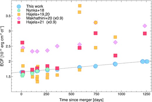
Energy conversion factor (ECF) used to transform count rates into fluxes in the 0.3–10 keV band. Our results are compared with values derived from the literature (Nynka et al. 2018; Hajela et al. 2019, 2020; Makhathini et al. 2020; Hajela et al. 2021), highlighting substantial differences in the reported fluxes.
As shown in Fig. 2, we find a good agreement with the values of Nynka et al. (2018) and, partially, with those of Hajela et al. (2021) between 15 d and 260 d (Epochs 3–6 in Table 1). In other epochs, the work of Hajela et al. (2021) derives higher and highly variable ECFs, not consistent with our analysis. The net result is an higher average flux level at late times. A systematic discrepancy is also found with the values quoted in Makhathini et al. (2020, Table 1), which are consistently higher than our values by 40 per cent. Such large discrepancy is only found when using the flux densities at 1 keV reported in their Table 1. By comparing the fluxes of the single Chandra observations (our Table 2 and Table 2 in Makhathini et al. 2020), we find a good agreement between the two works. With respect to our previous analyses (Troja et al. 2017, 2018; Piro et al. 2019; Troja et al. 2019, 2020), we find consistent values and only note that the X-ray fluxes increased by 10 per cent the values in Troja et al. (2020) due to the updated calibration files used in this work.
In contrast to our method, which is based on the broadband (from radio to X-rays) spectral fitting of the afterglow data, Hajela et al. (2019) and Hajela et al. (2021) determine the spectral shape, and hence the ECFs, using only the X-ray data. This method has some advantages: it is independent from the afterglow model and potentially sensitive to the source spectral evolution, but in practice it is dominated by the large uncertainties of the low-counts regime. Nonetheless, for the sake of comparison, we also calculate the ECFs for the case of a time-variable spectral index. For several observations, and in particular those at early (<20 d) and late (>1 yr) times, we do not have sufficient photons for spectral analysis and we therefore use the hardness ratio to estimate the spectral shape (e.g. Evans et al. 2010).
We define the hardness ratio as HR = (H − S)/(H + S), where H and S are the net source counts in the hard (2.0–7.0 keV) and soft (0.5–2.0 keV) energy bands, respectively. Its late-time temporal evolution is shown in Fig. 3, updated from Troja et al. (2020) using the latest observations at ≈1230 d and the relevant calibration files. We still assume an absorbed power-law model with NH fixed to the Galactic value and variable photon index Γ. Following Evans et al. (2010), we input the spectral model and response files into the CIAO tool modelflux and create a look-up table of hardness ratios and ECFs by stepping Γ from 0 to 3 in steps of 0.1 and recording at each step the model count-rates and fluxes in different bands, namely 0.5–2.0 keV (soft), 2.0–7.0 keV (hard), and 0.5–7.0 keV (broad). We then derive the observed hardness ratio following Park et al. (2006), and infer the corresponding photon index and ECF from the look-up table. The 68 per cent confidence level uncertainty on the HR is used to estimate the error on the ECF. Using data from Epoch 4 (t=109 d), when the afterglow is sufficiently bright for an independent spectral analysis, we verify that the photon indices, Γ = 1.6 ± 0.2 from the HR and Γ = 1.66 ± 0.17 from the spectral fit, are in good agreement.
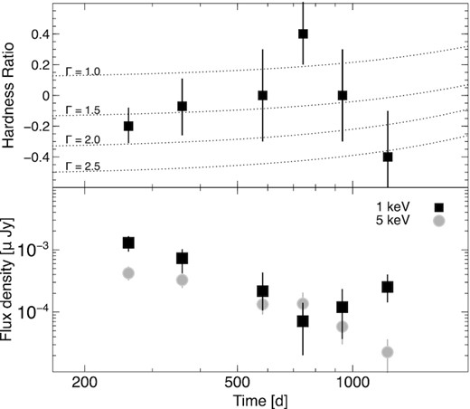
Top panel: temporal evolution of the hardness ration HR. Dotted lines show the values expected for an absorbed power-law model with photon index Γ between 1.0 and 2.5, and take into account the evolving instrumental response. Bottom panel: X-ray flux light curves at 1 keV (squares) and 5 keV (circles) derived using a time-variable photon index inferred from X-ray observations. The apparent rise of the soft X-ray emission (1 keV) is a result of the hard-to-soft spectral evolution seen at late times.
The resulting ECFs and X-ray fluxes, calculated for a time-variable photon index, are listed in Table 1 in the ‘Γ free’ columns. Although this method yields a better agreement with the results of Hajela et al. (2021), it cannot reproduce the increase in flux at 1230 d. For the range of spectral indices Γ ≈1-2 typical of an afterglow, variations in the ECFs are ≲20 per cent. Spectral variations, unless extreme, do not significantly affect the flux estimates, but can have a noticeable impact on the derived flux densities, as shown in the bottom panel of Fig. 3. For a central energy of 1 keV, the conversion factor from rate to flux density increases by 65 per cent between Γ=1 and Γ=1.5, and more than doubles between Γ=1 and Γ = 2. By suppressing the flux density in the case of a hard spectrum and boosting it in the case of a soft spectrum, the soft-hard-soft evolution seen in the HR diagram is at the origin of the apparent rise of the light curve at 1 keV. This temporal feature is not seen in either the count rate, the integrated flux or the flux light curve at 5 keV, which is less sensitive to spectral variations. It would therefore be inaccurate to interpret it as the onset of a new, spectrally harder component of emission as this trend appears only in the case of a significant (ΔΓ ≳0.5) hard-to-soft evolution of the X-ray spectrum.
Finally, we investigate whether instrumental artifacts, such as hot columns or bad pixels, lie close to the source position on the detector. These factors may cause large variations of the ECF, such as the one seen in Fig. 2. However, a visual inspection of the exposure maps shows that they do not affect the observations of GW170817. As seen in Fig. 6, the combined exposure maps for the latest observations show that the target was observed in optimal conditions. We therefore do not expect large variations of the ECF between the different observations.
2.1 Constraints from radio observations
We monitored the target using the Australian Telescope Compact Array (ATCA; project C3240, PI: L. Piro) between November 2020 and April 2021. Our observations span the frequency range 2.1–9.0 GHz and are reported in Table 3. The radio counterpart is not detected and we place a 3 σ upper limit of ≲ 31 μJy at 9 GHz.
Radio observations were also carried out with the Jansky Very Large Array (VLA) between September 2020 and February 2021, as reported in Balasubramanian et al. (2021). No signal is detected by combining ≈30 h of imaging at 3 GHz. By performing forced photometry at the GRB position, Balasubramanian et al. (2021) reports a flux of 2.9 ± 1.0 μJy. We independently analyzed the public available dataset, carried out under programs SL0449 and SM0329 (PI: Margutti), totalling 12 h of observing time in S-band (of which ≈ 10 h on-source) and 4 h in Ku-band (of which ≈2.3 h on-source). The VLA visibility data were downloaded from the NRAO online archive and calibrated with the CASA VLA pipeline v1.3.2. The splitted calibrated measurement sets from the three A-array S-band datasets (MJD 59198, 59210 and 59247) of GW170817 were merged via the CASA task concat and imaged interactively using the CASA task tclean with robustness parameter set to 0.5. Our results are listed in Table 3. The restored image is characterized by an rms of ≈1.9 μJy (3 GHz) measured via the CASA task imstat in a region of the cleaned map away from sources. A similar value of ≈1.7 μJy is measured in the Ku-band (15 GHz). At the position of GW170817, any visible signal is consistent with the noise level. At the transient position we find a peak force-fitted flux density of 3.1μJy/beam. Our analysis is in agreement with the weak radio flux inferred by Balasubramanian et al. (2021) and shows no evidence of a rebrightening in this band.
We use XSPEC v.12.11.1 (Arnaud 1996) to perform a joint fit of the latest X-ray and radio data (Fig. 4). Our upper limits constrain the power-law spectral index β = Γ-1 to ≲1.6. The tentative radio detection of Balasubramanian et al. (2021) yields β = 0.54|$^{+0.02}_{-0.03}$|, slightly harder but consistent (within the 95 per cent confidence level) with the value of 0.585 derived from afterglow spectroscopy at earlier times (Troja et al. 2019). Using this best fit model, the X-ray flux in the 0.3-10 keV band is 1.8|$^{+0.5}_{-0.6}$| × 10−15 erg cm−2 s−1, fully consistent with the value estimated in Table 1 (Epoch 11) and 30–40 per cent lower than the flux quoted in Hajela et al. (2021). The low signal-to-noise of the radio and X-ray data does not allow us to place any strong spectral constraint. The slightly harder radio-to-X-ray index as well as the softer X-ray spectrum seen in the HR diagram are both features of marginal statistical significance (≈2 σ and ≲1 σ respectively).
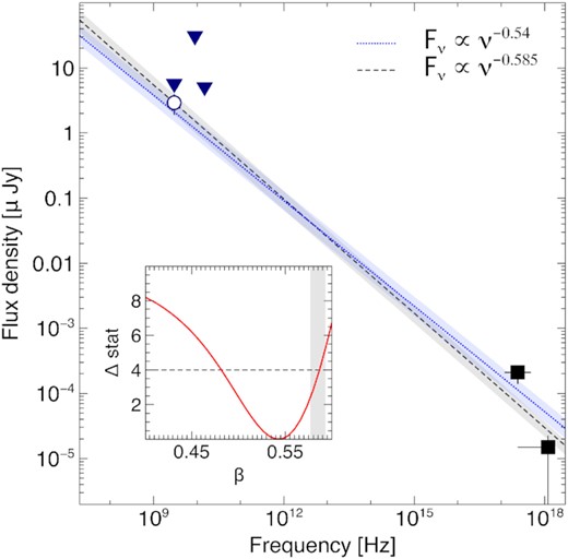
Spectral energy distribution of the late time (≈1230 d) afterglow compared with two power-law models with index 0.54 (dotted line) and 0.585 (dashed line). The 3 σ radio upper limits (downward triangles) at 3 GHz, 9GHz and 15 GHz and the X-ray fluxes are derived from our analysis. The radio flux (open circle), corresponding to a marginal detection at 3 GHz, is from Balasubramanian et al. (2021). The contour plot for the spectral index is shown in the inset. The afterglow value of 0.585 ± 0.005 is marked by the vertical bar.
If the joint radio/X-ray analysis is performed in flux space, discrepancies in the flux calibration might explain the different results reported in Hajela et al. (2021) as well as the harder spectral index derived in Makhathini et al. (2020). Our fit to the X-ray data is performed in count space and does not depend on the flux calibration given in Table 1, but is consistent with it.
3 COMPARISON TO THE JET MODEL
Fig. 5 compares the updated dataset with the jet model presented in Troja et al. (2020), who fit the dataset of the first 10 epochs (≲ 940 d) with a Gaussian structured jet. We have used the MCMC samples from these fits to construct posterior distributions of the model flux at 940 (Epoch 10), 1212 (Epoch 11a), 1255 (Epoch 11b), and 1234 (Epoch 11) d after the burst. We convert the flux predictions into counts by using the ECF (Table 1, col. 5) and a background level of ≈7.8 × 10⁻⁶ cts s−1 within the aperture. The posterior predicted number of counts for each observation are 5, 3, 3, and 6 respectively. The corresponding observed photon counts are 8, 10, 5, and 15. Assuming Poissonian statistics, for each epoch we compute the probability of observing a count at least as high as the true observation, marginalized over the posterior distribution to account for uncertainty in the fit. The 1208 d (Epoch 11a) observation displays the most significant deviation at ≈3σ (Gaussian-equivalent; statistical only). Combining Epochs 11a and 11b into Epoch 11 at 1232 d still results in a ≈3 σ excess over the Troja et al. (2020) model fit. Epochs 11b (at 1255 d) and 10 (at 940 d) show more modest excesses of ≈1.2σ each. These are all over-estimates of the excess over this particular jet-only model, as they do not take into account uncertainties in the calibration or modeling.
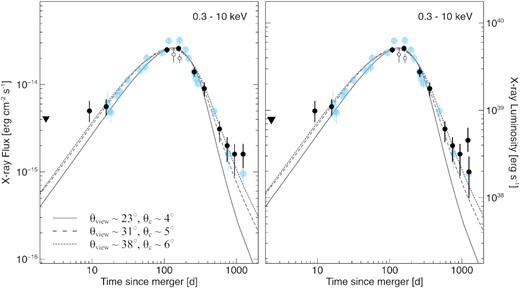
X-ray (black circles: Chandra; open circles: XMM-Newton) light curves compared with the jet model of Ryan et al. (2020) (solid line), Troja et al. (2020) (dashed line), and this work (dotted line). Radio data (blue; Makhathini et al. 2020; Balasubramanian et al. 2021) at 3 GHz were rescaled using a spectral slope of 0.585. At late times a deviation from the jet model is visible. By rebinning the last two Chandra observations (left-hand panel), the X-ray emission seems to flatten. This effect is mostly driven by the detection of soft (<2 keV) X-ray emission at 1211 d, visible in the unbinned light curve (right-hand panel).
We have also performed an updated jet model fit including the new observations at T > 1200 d. The jet model is identical to that in Troja et al. (2020), a Gaussian structured jet computed with afterglowpyv0.6.5 (Ryan et al. 2020). With the new observations included in the fit the significance of the late time excess is reduced, as expected, at the cost of increasing tension with VLBI observations. Our values are lower than the significance reported by Hajela et al. (2021), showing that systematic uncertainties in the modeling of the afterglow evolution as well as in the estimates of the X-ray flux need to be taken into account. As shown in Fig. 2, the higher ECF values used by Hajela et al. (2021) at late times lead to higher fluxes as well as a rising temporal trend, which is not observed in count space: in both epoch 10 (940 d) and 11 (1230 d), the source is detected at a level of 0.8 × 10⁻⁴ cts s−1.
The new data confirm the trend observed in Troja et al. (2020), a structured jet model can explain the observed X-ray emission if viewed at a larger angle than previously estimated. The relative excess of the late-time X-ray observations can be accounted for by a wider jet, which has a larger total energy. Since the afterglow’s early rise at T < 160 d fixes the ratio of the viewing angle to the jet opening angle (Ryan et al. 2020; Nakar & Piran 2021), the wider jet must be viewed proportionally further off-axis. The new fit estimates the viewing angle θv = 38° ± 4°, larger than the 31° ± 5° reported in Troja et al. (2020) with 1000 d of data and the 23° ± 6° reported in Troja et al. (2019) and Ryan et al. (2020) with 1 year of data. As a consequence of the larger viewing angle, the associated superluminal apparent velocity shifts from βapp = 2.2|$^{+0.5}_{-0.4}$| to |$\beta _{app} = 2.0^{+0.3}_{-0.2}$|, increasing further the tension with the value of β = 4.0 ± 0.5 determined by the VLBI centroid motion, from |$2.8\, \sigma$| (Troja et al. 2020) up to |$3.5\, \sigma$| when marginalized over the fit. As noted in Troja et al. (2020), the addition of an extra-component with luminosity LX ≈ 2 × 1038 erg s−1 would resolve this tension. With the additional component making up the late-time emission, the underlying jet is allowed to be narrower and nearer the line of sight, with an opening angle of θc = 4° ± 1° and viewing angle θv = 26° ± 6°. This alignment produces an apparent velocity of |$\beta _{app} = 3.1^{+0.9}_{-0.6}$|, in agreement with the measurement of Mooley et al. (2018).
Although our analysis confirms that the X-ray and radio emission deviate from early predictions of the jet model with θv ≈20°, the interpretation of this late-time behaviour remains ambiguous. The flattening of the X-ray light curve, seen in the left-hand panel of Fig. 5, is suggestive of an additional component taking over the fading GRB afterglow. Although tantalizing, the observed trend is driven mostly by a single data point at 1211 d, deviating ≲3 σ from the afterglow predictions (right-hand panel of Fig. 5), and a continued fading of the X-ray and radio counterpart remains consistent with the observations. Uncertainty in the background contribution might further decrease the significance of the X-ray excess.
In Troja et al. (2020), we already discussed in detail the possible origins of the late-time X-ray emission and made predictions about its future evolution. Here we briefly review them in light of the new observations. A deviation from the simpler jet model could be caused by a change in the jet dynamics. In the current phase of evolution the jet is trans-relativistic and undergoing lateral spreading. As noted by Troja et al. (2020), a mere factor of four in density change beyond a parsec would lead to a factor of two increase in flux, both in the relativistic and non-relativistic regimes. During spreading, models in the relativistic limit show the flux to be effectively insensitive to density (Fν ∝ n(3 − p)/12, Granot et al. 2018; Hajela et al. 2021), implying a far more drastic gradient to reproduce the observed flux. On the other hand, this would in turn hasten the onset of the non-relativistic stage where Fν ∝ n0.4 (Leventis et al. 2012).
Evolution in the properties of the non-thermal electrons, for instance a decrease in the electron index p towards the expected non-relativistic value of 2 (Bell 1978; Blandford & Ostriker 1978) as the jet decelerates, could in principle increase the X-ray flux above the fixed-p predictions of our current models. However, the full behaviour of the electron population in such an evolving-p scenario is unknown, so no robust predictions, even whether the X-ray flux would increase or decrease, are possible at this time.
An exciting possibility would be emission from the counter-jet – the one pointing out in the opposite direction (Li et al. 2019). As shown in Troja et al. (2020), this does not arise with natural parameters – that is with a jet and circumburst medium with similar properties to those observed in our direction. Although we expect the outflow to be bipolar, the minimum angle between the two jets may be less than 180 degrees due to slightly different local conditions at jet launch on either side of the merger remnant (Liska et al. 2018; Ruiz et al. 2020). However, any deviation from axial symmetry may be too small to explain an early counter-jet appearance. In order to be visible the counter jet must slow down faster than the jet pointing towards us, either because of a significant density gradient in the opposite direction or possibly a lower counter-jet energy (Nakar, priv. comm.).
The most natural scenario is the onset of the late time flare arising from the interaction of the merger ejecta with the surrounding matter (Nakar & Piran 2011). This signal would rise on a time scale comparable to the observation time scale with a rising slope that depends on the velocity profile of the ejecta m(v) (Nakar & Piran 2011; Piran, Nakar & Rosswog 2013; Hotokezaka & Piran 2015). To avoid quenching by the jet blast wave (Margalit & Piran 2020; Ricci et al. 2021), this model would require a small amount ∼10−5 M⊙ of fast moving ∼0.8c material to be ejected along the polar axis. This high velocity could also explain the relatively early appearance of this signal. The spectrum of this new component should be more or less similar to the jet afterglow spectrum as the physics of the shocks that produce both is similar. Still some minor spectral changes are reasonable, but in particular we should expect a comparable or even higher increase in the radio band which, at present, is not observed.
An alternative possibility is emission from the central compact object. The scenario of a long-lived NS was already discussed in Troja et al. (2020), Piro et al. (2019), and references therein. This model predicts a flattening of the late-time emission as a possible signature of the inner engine. If this signal is powered by the NS spindown energy, the observed timescales imply a poloidal field B ≈1011-1012G, consistent with the limits set by the broadband observations (Ai, Gao & Zhang 2020).
There are two possibilities for such a scenario: one is that the external shock is continuously energized by the pulsar wind (Zhang & Mészáros 2001), which also predicts an achromatic signature between X-ray and radio bands. Alternatively, X-ray emission can be produced by the internal dissipation of the pulsar wind, which would not predict a simultaneous re-brightening of the radio flux (Troja et al. 2007). If such a chromatic behaviour is observed, it would lend strong support to the existence of a late central engine. Short timescale X-ray variability would be another key signature for this model.
As the last X-ray detection appears rather soft in spectrum (Fig. 3) and its luminosity is comparable to the Eddington luminosity of a solar mass object, another possibility would be X-ray emission from fallback matter (Rosswog 2007; Rossi & Begelman 2009). In the latter case, the expected spectrum would be approximately thermal, peaking in the soft X-rays (≲2.0 keV) and with a negligible radio signal. One can expect this component to decrease slowly on a time scale dictated by accretion processes or by the fallback rate. In this model, the central compact object can be either an NS or a solar-mass black hole.
Given the faintness of the source, it could be difficult to discern between different models unless the emission flattens at the current level, as envisioned in Piro et al. (2019), or starts to rise as in the ‘radio flare’ scenario (Nakar & Piran 2011).
4 CONCLUSIONS
We present a comprehensive analysis of the X-ray emission from GW170817 and find that the latest observation deviate from the simple jet model, confirming the trend already noted in Troja et al. (2020) and more recently discussed in Balasubramanian et al. (2021) and Hajela et al. (2021). This is a robust trend, which does not depend on a single observation, but has been consistently observed at X-ray and, to a less extent, radio energies for several months.
If interpreted as arising from the same jet that produces the afterglow so far, the recent data increases the tension (from 2.8 σ to 3.5 σ) between the observed temporal profile, which continues to favour large viewing angles θv ≳ 30°, and the constraints placed by the VLBI centroid motion, which instead points to θv ≲ 20°.
Alternatively, the late-time data may indicate a new component of emission, arising from the central compact object or from the long predicted flare (Nakar & Piran 2011) expected from the interaction of the ejecta with the surrounding matter. This interpretation would require some fast ∼ 0.8c moving matter that probably arose from the dynamical ejecta.
However, we also highlight how systematic uncertainties in the calibration and modeling of the data may affect the conclusions. In particular, we do not find evidence of a rising X-ray emission in either count or flux space. Similarly, we do not find any statistically significant spectral change. The behaviour of the late-time afterglow remains open to multiple interpretations, and continued monitoring at radio and X-ray wavelengths is key to identify the origin of such long-lasting emission from GW170817.
SUPPORTING INFORMATION
Figure S1. Exposure maps for the last three sets of Chandra observations, performed around 940 d (Epoch 10 in Table 1), 1212 d (Epoch 11a), and 1255 d (Epoch 11b) after the merger.
Table S2. Log of y X-ray observations of GW170817.
Table S3. Flux densities from the latest radio observations of GW170817 by ATCA and VLA. The upper limits are at the 3σ level.
Table S4. Observed X-ray fluxes in the 0.5-7.0 keV energy band.
Please note: Oxford University Press is not responsible for the content or functionality of any supporting materials supplied by the authors. Any queries (other than missing material) should be directed to the corresponding author for the article.
ACKNOWLEDGEMENTS
We thank the referee for insightful comments. ET and BO were supported in part by the National Aeronautics and Space Administration (NASA) through grants NNX16AB66G, NNX17AB18G, and 80NSSC20K0389. ET further acknowledges support from the National Science Foundation (NSF) award 2108950. LP and HJvE acknowledge support from the European Union’s Horizon 2020 Programme under the AHEAD2020 project (grant agreement number 871158). LP was supported in part from MIUR, PRIN 2017 (grant 20179ZF5KS). TP was supported by an advanced ERC grant TReX.
DATA AVAILABILITY
The data underlying this article will be shared on reasonable request to the corresponding author.
