


ABSTRACT
Observation of redshifted 21-cm signal from the Epoch of Reionization (EoR) is challenging due to contamination from the bright foreground sources that exceed the signal by several orders of magnitude. Removal of this very high foreground relies on accurate calibration to keep the intrinsic property of the foreground with frequency. Commonly employed calibration techniques for these experiments are the sky model-based and the redundant baseline-based calibration approaches, which can suffer from sky-modelling error and array redundancy imperfection respectively. In this work, we introduce the hybrid correlation calibration (CorrCal) scheme, which aims to bridge the gap between redundant and sky-based calibration by relaxing redundancy of the array and including sky information into the calibration formalisms. We apply the CorrCal to the data of Precision Array for Probing the Epoch of Reionization (PAPER) experiment, which was pre-calibrated using redundant baseline calibration. We show about |$6\%$| suppression at the bin right on the horizon limit of the foreground wedge-like structure, relative to the pre-calibrated power spectra. This small improvement of the foreground power spectra around the wedge limit could be suggestive of reduced spectral structure in the data after CorrCal calibration, which lays the foundation for future improvement of the calibration algorithm and implementation method.
1 INTRODUCTION
The cosmic dark ages ended at around 100 million years after the big bang, marking the formation of the first structures such as galaxies and stars. These objects started to emit radiation that influences the nearby primordial intergalactic medium (IGM), which predominantly filled with the neutral hydrogen atom. As the number of these very first sources increases, they emitted sufficient radiation to convert the neutral IGM into the fully ionized medium of the hydrogen atom eventually. The period that marks the transition of neutral IGM into the fully ionized state is known as the Epoch of Reionization (EoR) in the history of the Universe. Thus, investigating the era of EoR will answer the fundamental questions of the formation of the first structures and their properties.
The measurement of the radiation from the high-redshifted 21-cm emission line is employed to probe the EoR era. This emission line is due to the hyperfine transition of the neutral hydrogen atom in the IGM empowered by the first sources. The information imprinted into the radiation associated with the redshifted 21-cm line can be used as a powerful tool in the modern cosmology to study the ionization state and large-scale temperature fluctuation of IGM, owing to the formation of the first structures (see e.g. Barkana & Loeb 2001; Oh 2001; Furlanetto, Oh & Briggs 2006; Morales & Wyithe 2010; Pritchard & Loeb 2012).
A direct probe of the EoR is the tomographic mapping of redshifted 21-cm signals from the neutral hydrogen atom (Madau et al. 1996; Barkana & Loeb 2001; Furlanetto et al. 2006; Morales & Wyithe 2010; Pritchard & Loeb 2012). Significant progress has made in the past decades, because several experiments dedicated to studying this signal have been built or are being upgraded. The first-generation 21-cm experiments, including the Murchison Widefield Array (MWA; Tingay et al. 2013), the Donald C. Backer Precision Array for Probing the Epoch of Reionization (PAPER; Parsons et al. 2010), the LOw-Frequency ARray (LOFAR; van Haarlem et al. 2013), and the GiantMeter wave Radio Telescope EoR experiment (GMRT; Paciga et al. 2011) are already operating and taking data. Observations from these first-generation experiments have set upper limits to the statistical power spectrum of 21-cm brightness temperature from cosmic reionization. In particular, results from MWA, LOFAR, and PAPER observations (e.g. Paciga et al. 2011; Dillon et al. 2014; Patil et al. 2017; Cheng et al. 2018; Kolopanis et al. 2019; Mertens et al. 2020) have placed upper limits on the statistical power spectrum of the 21-cm emissions over a broad range of redshifts, providing evidence for the heating of the IGM before reionization. The most recent result from MWA constrained the EoR power spectrum as |$\Delta ^{2}=(43\, {\rm mK})^{2}=1.8 \times 10^{3}\, {\rm mK}^{2}$| for |$k=0.14\, h\, {\rm Mpc}^{-1}$| at z = 6.5, which is the tightest measurement currently (Trott et al. 2020; Rahimi et al. 2021). Lessons learned from these experiments have led to the construction of the second-generation instruments, which include the Hydrogen Epoch of Reionization Array (HERA; DeBoer et al. 2017), the upgraded MWA (MWA-II; Wayth et al. 2018), and the LOFAR 2.0 Survey (Edler, de Gasperin & Rafferty 2021). With more collecting areas and improved electronics, high-significant measurements of the 21-cm power spectrum are anticipated from these second-generation instruments (Pober et al. 2014; Liu & Parsons 2016; Wayth et al. 2018).
Detecting the 21-cm signal from EoR is challenging due to the weakness of 21-cm signal comparing to the brightness temperature of the foreground originated from synchrotron radiation from our Galaxy, strong point sources, and thermal bremsstrahlung from the H ii region (Shaver et al. 1999; Santos, Cooray & Knox 2005; Furlanetto et al. 2006; Bernardi et al. 2009; Parsons et al. 2014). To disentangle strong foregrounds from weak 21-cm signal, several mitigation techniques have been developed (see e.g. Wang et al. 2006; Bowman, Morales & Hewitt 2009; Liu et al. 2009; Liu & Tegmark 2011; Parsons et al. 2012; Dillon, Liu & Tegmark 2013; Liu, Parsons & Trott 2014a; Beardsley et al. 2016; Pober et al. 2016; Hothi et al. 2021). These techniques, in general, can be categorized into two approaches – foreground subtraction and foreground avoidance (Chapman & Jelić 2019). Foreground subtraction involves modelling of the foreground and subtracting them from the data. In contrast, foreground avoidance completely discards foreground contaminated data from analysis and tries to reconstruct the power spectra of EoR in the Fourier regime, which are not affected by foreground.
In both foreground mitigation and subtraction, accurate calibration of the array is critical because calibration errors can contaminate the Fourier mode of the EoR power spectrum (Morales et al. 2012; Ewall-Wice et al. 2017). Furthermore, simulations in Orosz et al. (2018) suggested that calibration error introduced by quasi-redundancy in antenna positioning and slight variations of the beam responses between different antennas are significant sources of contamination of the EoR signal. Even in the limit of perfect antenna positioning and telescope response, the EoR window can still be contaminated if the instrument calibration is susceptible to sky-modelling error (Byrne et al. 2019).
The array configuration of PAPER is designed to enhance sensitivity for a first power-spectrum detection by measuring same Fourier modes on the sky with a group of redundant baselines. These redundant visibilities need to be calibrated accurately by using the redundancy information of the array. The calibration technique implemented for such kind of array layout is generally known as redundant baseline calibration (Wieringa 1992; Liu et al. 2010). This technique intends to calibrate measurements from the array of antennas configured on a regular grid spacing with maximum redundancy in baseline distribution and tightly packed with the drift-scan mode of observations. Then one can use statistical tool to calibrate the visibilities for independent baselines.
In this work, we introduce a recently developed calibration scheme called correlation calibration (CorrCal1), first proposed in Sievers (2017). CorrCal aims to bridge the gap between sky-based and redundant calibration by incorporating partial sky information and information on the non-redundancies of the array into the calibration solutions. We use this new scheme to re-calibrate data from the 64-element PAPER array (hereafter PAPER64), which is a 9-h integration data set. Ali et al. (2015) calibrated this data set with a redundant baseline calibration scheme and published power spectrum results. This work used the same initial calibration techniques employed in Ali et al. (2015) but has an independent pipeline from that point on. We will show that CorrCal can potentially constrain the wedge-like structure of foreground in the Fourier space.
The rest of paper is organized as follows. In Section 2, we give a general review of common calibration approaches for radio interferometric measurements. In Section 3, we present CorrCal calibration scheme. In Section 4, we apply our method to the 9-h PAPER-64 data set. In Section 5, we present the results of the CorrCal calibration. The conclusion will be in the last section.
2 A REVIEW OF CALIBRATION FORMALISM
In radio interferometry, the correlated signal (visibility) from two independent receiving elements (antennas) is the sum of the system noise and the actual sky signal (or true sky visibility) multiplied by the complex gain parameters of the antennas. The gain parameters depend on the electromagnetic properties of the antennas, whereas the additive noise is mostly dominated by the thermal noise of the receiver system and the sky components.
Most calibration software packages developed so far to solve for the gain parameter |${\bf \textsf {G}}$| can be categorized into either one of the two conventional approaches, i.e. sky-based calibration or redundant-baseline calibration.2 In the sub-sections that follow, we present the underlying mathematical formalism of these two calibration approaches and discuss their inherent advantages and disadvantages.
2.1 Sky-based calibration
2.2 Redundant calibration
Due to the degeneracies in the measurement equation (equation (7)), the least-square estimator of equation (8) will not converge to a unique solution. Here, the term degeneracies refers to the linear combinations of gains and visibilities that redundant calibration cannot solve for, which results in the χ2 function invariant across different choices of the degenerate parameters. In-depth discussions of degeneracy issues in redundant baseline calibration can be found in Liu et al. (2010), Zheng et al. (2014), Dillon et al. (2018), and Byrne et al. (2019).
In general, redundant baseline calibration suffers from four types of degeneracies for array elements configured on the same plane. First, if one multiplies the amplitude of the antenna gain by a constant factor A and divides the sky parameter by A2, the χ2 remains unchanged so that the overall amplitude, A, of the instrument cannot be solved. Secondly, moving the phase of the gain parameter by certain amount Δ, i.e. |$g_{p}=|g_{p}|e^{j\phi _{p}}\rightarrow |g_{p}|e^{j(\phi _{p}+\Delta)}$| does not affect the χ2 due to the cancellation of |$g_{p}\times g^{*}_{q}$| in equation (1). The third and fourth degeneracies are caused by phase gradients Δx and Δy along x and y directions, respectively, for a planar array. For example, if one shifts |$g_{p}=|g_{p}|e^{j\phi _{p}}\rightarrow |g_{q}|e^{j(\phi _{q}+\Delta _{x}x_{q}+\Delta _{y}y_{q})}$|, it does not affect the χ2 if it is complemented by shift in sky parameter |$V_{pq}^{\rm {true}}=|V_{pq}^{\rm {true}}|e^{j\phi _{pq}}\rightarrow |V_{pq}^{\rm {true}}|e^{j(\phi _{pq}-\Delta _{x}b_{x}-\Delta _{y}b_{y})}$|, where xq and yq are the coordinates for antenna j, and bx = xq − xp and by = yq − yp are x and y coordinates of a baseline vector b connecting antenna p and q, respectively. So, the phase gradients Δx and Δy are still degenerate in the relative calibration stage. In a sense, inclining the whole array in either direction (x or y) is exactly equivalent to moving the phase centre of the sources on the sky in opposite direction. Hence, these two effects can cancel each other and result in the phase-gradient degeneracies, which in turn results in the sources appearing to be offset from the phase centre.
To fix the degeneracy issues, the redundant calibration can be divided into two calibration steps. These are relative calibration and absolute calibration. First, relative calibration is performed using the algorithm that we have just described to solve the antenna gains and the true sky. However, these solutions are degenerate, and an overall amplitude, an overall phase, and phase gradient calibration parameters remain unknown. Then, absolute calibration is performed to set these degeneracies to a reference and obtain the final calibration solutions. One particular approach for absolution calibration, as discussed in Byrne et al. (2019), is to map a pre-defined sky model of bright point sources to the degenerate parameters. However, setting degeneracies using the sky information in redundant calibration is difficult because incompleteness of the sky model can introduce frequency-dependent gain errors, which may lead to spectral structures in the otherwise smooth observations (Barry et al. 2016; Byrne et al. 2019).
Thus, the fundamental shortcomings of redundant calibration are imperfection of array redundancy and sky-modelling error. During the absolute calibration stage, the sky-modelling error enters into the redundant calibration. Redundant calibration assumes that the same sky is seen by all baselines in the same redundant group, requiring these baselines to have the same physical length and orientation. This assumption also dictates that all antenna elements in the array have the same primary beam responses. In the real situation, both are impossible to achieve for the level of accuracy required. These non-redundancies will result in calibration errors that lead to more foreground contamination in the cosmological Fourier space for 21-cm signal (Ewall-Wice et al. 2017; Orosz et al. 2018). The powerful alternative is to include the relaxed-redundancy information and position of sources into the calibration formalism (Sievers 2017).
3 CORRELATION CALIBRATION (CORRCAL)
Sievers (2017) proposed a hybrid calibration scheme called CorrCal, which aims to further bridge the gap between sky-based and redundant calibrations by taking into account sky and array information into the calibration algorithm. The CorrCal framework relies on the assumption that sky information is statistically Gaussian, which is a good approximation (Sievers (2017)). This assumption allows CorrCal to relax the redundancy of the array and including the known sky information in its formalism through covariance-based calculation of χ2. The covariance matrix thus forms a statistical model of the sky power spectrum, weighted by the instrumental response. We describe the underlying mathematical formalism of CorrCal in this section.
For the sake of computational tractability, the implementation of the Woodburry inversion to equation (23) in CorrCal follows the following steps:
First, the Woodburry inversion can be applied to Γ−1, where |$\Gamma = ({\bf \textsf {N}}+\hat{{\bf \textsf {r}}}\hat{{\bf \textsf {r}}}^{\dagger})$| for each redundant group separately, ignoring the source vectors |${\bf \textsf {s}}$|. To apply Woodburry identity to Γ−1, let |${\bf \textsf {B}}={\bf \textsf {N}}$| and |${\bf \textsf {v}}={\bf \textsf {r}}$|. Then, the inverted form of Γ is kept separate for each redundant group and saved in a factored form by applying the Cholesky factorization of the matrix |$[{\bf \textsf {I}}+{\bf \textsf {v}}^{\dagger }{\bf \textsf {B}}^{-1}{\bf \textsf {v}}]^{-1}$| in equation (24) for the redundant vectors |${\bf \textsf {r}}$|.
Finally, using the source vectors |${\bf \textsf {s}}$|, and the already factored form of Γ−1 from the first step, the Woodburry inversion can be computed using |$(\Gamma +\hat{{\bf \textsf {s}}}\hat{{\bf \textsf {s}}}^{\dagger })^{-1}.$|
3.1 Determining the sky and noise variance–covariance matrices
To perform the CorrCal, we first need to estimate the matrices |${\bf \textsf {R}}$|, |${\bf \textsf {S}}$|, and |${\bf \textsf {N}}$|. Thus, in this section, we will derive these variance–covariance matrices explicitly.
3.1.1 Diffuse sky component matrix (|${\bf \textsf {R}}$|)
For an instrument with a small field of view, the covariance matrices can be directly constructed from the visibility in the two-dimensional (2D) UV plane. However, most 21-cm experiments, including PAPER, use receiving elements that have wide field of views. Thus, the curvature of the sky becomes important. To account for this effect and simplify the calculation, we will first project the visibility function into the spherical harmonic space before calculating the covariance.
We calculated the array function that is defined in equation (26) using the exponential argument (|${\boldsymbol {b}}\cdot \hat{{\boldsymbol {r}}}{}/c$|) in equation (25) and the PAPER-64 beam model depicted in Fig. 2. The simulated exponential argument is shown in Fig. 1 for the PAPER-64 baselines oriented along the East–West and the North–South directions. To generate the beam model of the PAPER-64 array within the frequency range of 120 –168 MHz, we use the Astronomical Interferometry in Python (AIPY),4 a software package primarily developed for PAPER/HERA data analysis. Fig. 2 shows that the AIPY-simulated PAPER-64 beam model projected on the HEALPIx5 coordinates at three arbitrary right accessions for frequency of 150 MHz. We will use this beam model for all calculations of the covariance matrices.
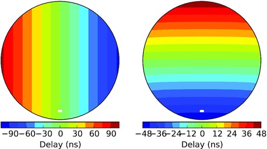
A delay term (|${\boldsymbol {b}}\cdot \hat{\mathbf {r}}/c$|) pattern in nanoseconds (ns) over PAPER latitude for baselines pointed along the East–West (left) and the North–South (right) directions. These baselines are calculated from the actual PAPER-64 antenna coordinates that are shown in Fig. 8.
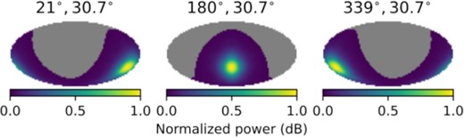
The AIPY-simulated antenna beam pattern of PAPER-64 array at 150 MHz at different longitudes, plotted for the PAPER latitude (30.7○S) at Karoo desert, South Africa.
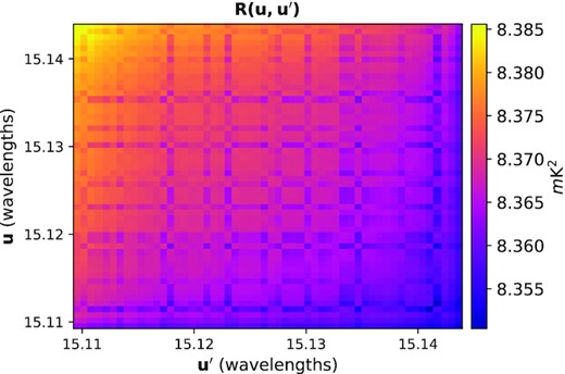
Covariance matrix between baselines obtained from the diffuse sky component at |$150\, {\rm MHz}$| for a redundant group containing about 30-m length baselines. The axes of this figure spanning the true measured variation in the baseline lengths for the baselines in the 30-m group. The entries of the covariance are not precisely equal as displayed in the figure. The covariance between baselines drops off as baselines become less redundant.
To pull |$C^{\rm diff}_\ell (f,f^{\prime })$| out of the summation sign in equation (32), we assume that for a given redundant block α, the sky is slowly changing function of ℓ ≈ 2π|u|. In other words, this means that the angular power spectrum of the sky does not evolve significantly over the baseline length within the redundant group.
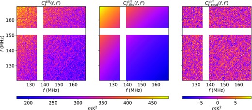
Left: Cross-frequency sky power spectrum |$C_{\ell }^{{\rm diff}}(f,f^{\prime })$| obtained from equation (34). Middle: The fitted power spectrum |$C_{\ell ,{\rm fits}}^{{\rm diff}}(f,f^{\prime })$|. Right: The residuals |$C^{\rm diff}_{\ell ,\rm resd}(f,f^{\prime })=C_{\ell }^{{\rm diff}}(f,f^{\prime })-C_{\ell ,{\rm fits}}^{{\rm diff}}(f,f^{\prime })$|. In all plot, we assume that the ℓ-dependence of |$C^{\rm diff}_{\ell }(f,f^{\prime })$| is the same. The whiteout regions are corresponding to the flagged frequency channels from the data.
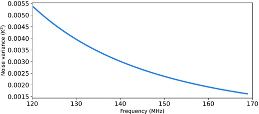
Noise variance estimated from the system temperature of PAPER.
We use equation (36) to represent the diffuse sky component for χ2 optimization process in equation (17). The dimension of the covariance matrix |${\bf \textsf {R}}$| depends on the number of baseline Nu and number of frequency channels Nf, i.e. its dimension is equal to NuNf × NuNf.
3.1.2 Point source component matrix (|${\bf \textsf {S}}$|)
The partial information about the point sources on the sky is one of the components the CorrCal calibration scheme employs to estimate the best likelihood antenna gain parameters. Simulation in Sievers (2017) showed that the inclusion of the bright sources information in CorrCal has a significant effect in reducing both amplitude and phase calibration error. However, the phase error has reduced remarkably (about a factor of 5 better than non-source-informed correlation calibration) when the correlation information of point sources has implemented in Sievers (2017), which substantially improves the quality of phase calibration.
In this study, we use the published astronomical catalogues in Jacobs et al. (2013) to model the known sources. Using sources information in this catalogue, we form the matrix |${\bf \textsf {S}}$| that carries the sources information.
3.1.3 Noise matrix (|${\bf \textsf {N}}$|)
3.2 Eigendecomposition of sky signal covariance matrix
However, for a quasi-redundant group, all the off-diagonal elements of the correlation matrix |${\bf \textsf {R}}$| are slightly different from one. As shown in Fig. 3, all the elements of the covariance matrix are not precisely equal. It shows that the correlation between baselines decreases as they become less redundant. In that case, we approximate |${\bf \textsf {R}}$| from its eigendecomposition in our analysis following Sievers (2017). If each redundant group in the array is not represented by few eigenmodes that are much less than the visibilities in the group, it shows that there is no sufficient redundancy in the array and therefore any calibration scheme that relies on the array redundancy may not give the accurate results. In the eigendecomposition analysis, few modes of the principal components accounted for most of the variances in the original data. Thus, those eigenmodes of |${\bf \textsf {R}}$| corresponding to sufficiently large eigenvalues could replace its original data with very little loss of information. In the left-hand panel of Fig. 6, we show the eigenvalues of cross-frequency covariance matrix described in equation (36). The vertical axis represents the log10 eigenvalues, while the horizontal axis labels the corresponding principal component numbers. The sharp falloff in the eigenvalues against the eigenmode index suggests that by measuring a few modes of an eigenvalue, one can account for most of the variation in the original data that forms |${\bf \textsf {R}}$|. In addition, all the eigenvalues are greater than zero because |${\bf \textsf {R}}$| is a positive-definite covariance matrix. In the right-hand panel of Fig. 6, we depict the first three eigenmodes for |${\bf \textsf {R}}$| corresponding to the first three eigenvalues for a frequency range from 120 to 168 MHz. Specially, the first and the second eigenmodes are more important to explain the diffuse sky covariance between frequency channel because they are a relatively smooth function of frequency.
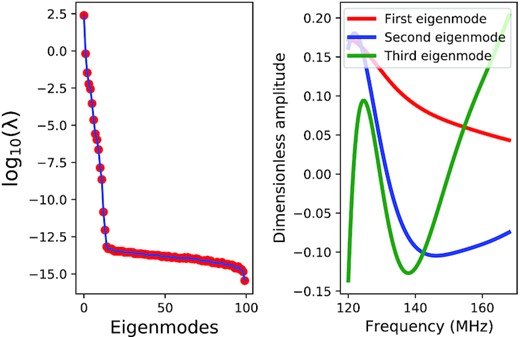
Left: Eigenvalues of cross-frequency covariance matrix described in equation (36). The vertical axis represents the log10 eigenvalues, while the horizontal axis labels the corresponding principal component index. Right: The first three eigenmodes for |${\bf \textsf {R}}$| corresponding to the first three eigenvalues for the frequency range from 120 to 168 MHz.
All off-diagonal elements of the noise variance matrix |${\bf \textsf {N}}$|, which has the same size as |${\bf \textsf {p}}\otimes {\bf \textsf {p}}^{\dagger }$|, are zero. Thus, Γ has only a relatively small number of non-zero elements and it can be considered to be sparse because most of its elements are zero. Therefore, it is wasteful to use the general dense matrix algebraic methods to inverting Γ since most of the O(N3) operations devoted to inverting the matrix involve zero operands. Hence, in terms of memory storage and computational efficiency, performing the sparse matrices operation traversing only non-zero elements has significant advantages over their dense matrix counterparts. Taking advantage of the sparse structure of the correlation matrix Γ, CorrCal utilizes the sparse matrix operations to increase its computational performance in a large data set.
To implement the sparse matrix computations in CorrCal, per-redundant group correlation matrices Γ are stored as sub-matrices on the diagonal of the square block-diagonal matrix. These sub-matrices will be square, and their dimensions vary depending on the number of baselines in the redundant group. Since the off-diagonal elements of the block-diagonal matrix are zero, and there can be many sparse sub-matrices stored as its diagonal elements, the overall matrix must be sparse. It can be easily compressed and thus requires significantly less storage, which also enhances the computational speed.
3.3 Implementation of CorrCal
The crucial steps to perform CorrCal are grouping data according to their corresponding redundant baseline and determining the matrices |${\bf \textsf {R}}$|, |${\bf \textsf {S}}$|, and |${\bf \textsf {N}}$| to each of these redundant groups. Then, one needs to set up the sparse matrix representations for these matrices and determine the χ2 function and its gradient information using the CorrCal routines. Utilizing these ingredients as inputs, CorrCal finally adopts the Scipy6 built-in optimization algorithm to fit antenna gains. We summarize the procedures of implementation of CorrCal as follows:
First, we need to create the sparse matrices representing |${\bf \textsf {R}}$|, |${\bf \textsf {S}}$|, and |${\bf \textsf {N}}$| set up to each redundant group using the CorrCal routine, sparse_2level(). The following arguments must be supplied to this routine to create sparse matrices:
The real-imaginary separated per-redundant group diffuses sky vector |${\bf \textsf {p}}$|. In this vector, we make all its entries equal to zero except those entries corresponding to eigenmodes that we kept per redundant block [see equation (46)].
The real-imaginary separated vector |${\bf \textsf {s}}$| that carries information about the known point sources.
Per-diagonal noise variance matrix |${\bf \textsf {N}}$|.
A vector that contains indices setting off the redundant group.
Secondly, the χ2 function and its gradient information should be determined using the CorrCal subroutines. The arguments passed to these sub-routines in order to calculate the χ2 function and the gradient information of χ2 are:
A vector containing the real-imaginary separated initial guess for antenna gains.
Per-redundant group measured visibility data vector. The real-imaginary parts should be separated such that imaginaries follow their respective reals [e.g. see vectorized visibility in equation (49)].
The sparse matrix representations for |${\bf \textsf {R}}$|, |${\bf \textsf {S}}$|, and |${\bf \textsf {N}}$| from the first step.
A vector containing per-visibility antenna indices.
Finally, using the χ2, its gradient information, and a vector of the initial guess for antenna gains that scaled by a large number as an input, CorrCal adopts the scipy built-in non-linear conjugate gradient algorithm, Scipy.optimize.fmin_cg(), to solve for antenna gains.
3.3.1 Antenna gain solutions as a function of frequency–bandpass solution
For the EoR studies, highly precise frequency-dependent bandpass calibration plays a crucial role. If one’s calibration solution has a noise-like structure along the frequency axis, it may introduce fine-frequency structure to the otherwise smooth sky observations even if the instrument’s response is the slow function of observing frequencies. It poses the serious challenges towards efforts to isolate spectrally structured weak 21-cm signal from spectrally smooth strong foreground signal. Several strategies have proposed for ensuring smooth calibration solutions as a function of frequency. For instance, simulation in Ewall-Wice et al. (2017) and Orosz et al. (2018) has shown that downweighting measurements from longer baselines in a redundant baseline calibration solution would eliminate the migration of fine spectral structure from longer baselines to the shorter baselines regimes. This effect is because the longer baselines have more chromatic nature than the shorter ones as shown in Morales et al. (2012). Other strategies fit the calibration solutions with smooth function in frequency for a bandpass calibration.
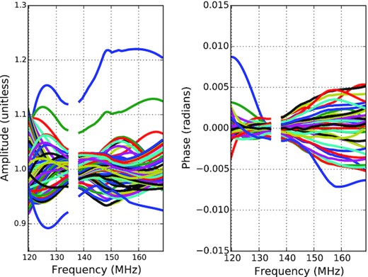
The bandpass gain solution derived from a snapshot of 10-min observation (JD2456242.25733) of PAPER-64 elements. Amplitude (left) and phase (right) of the gain solutions against frequency. Each line is a different antenna. Discontinuity in the gain solution shows the flagged frequency channel affected by RFI contamination.
3.4 Comparisons of CorrCal to other methods
The CorrCal approach has a distinct feature to alleviate issues like imperfections of array redundancy and miss-modelled sky catalogue that redundant baseline and sky-based calibration techniques suffer from. In CorrCal, sources with known positions can be included as a prior even if their fluxes are not precisely known, because the position of the sources is better known than their intensities during observation time and frequency. This concept allows CorrCal to assume that the source catalogue is complete and well modelled with precisely known source positions. The method works well if the sky-modelling error could be mostly caused by uncertain/missed source fluxes in the sky-based calibration approach.
The covariance-based formulation of χ2 in CorrCal provides significant flexibility by relaxing the assumption of explicit redundancy to accounts for imperfections of array redundancy. For instance, if baselines in a quasi-redundant group are assumed to be alike but they are not perfectly alike, then the CorrCal method incorporates this offset from perfection in its formalism by suppressing the off-diagonal elements of covariance matrix within the group. However, the redundant baseline method assumes that the baselines are perfectly redundant in the group, and therefore all the off-diagonal elements of the covariance matrix in the group are exactly equal [e.g. equation (42)].
4 THE PAPER-64 DATA SET
PAPER is a low-frequency radio interferometer experiment dedicated to probing the EoR through the measurements of the 21-cm power spectrum (Parsons et al. 2010). It was the first 21-cm array experiment with a redundant array configuration, where antennas were arranged in a regular grid to generate multiple copies of the same baselines. The redundant baselines probe the same modes on the sky, resulting in significant improvement in the sensitivity of the 21-cm power spectrum; thus, it is reasonable to use redundant calibration. The array was operating at the South African SKA site in the Karoo desert until its decommissioning in 2015. It was first deployed with 16 antennas and continued to grow, eventually increasing to 128 antennas in 2015. PAPER has 1024 frequency channels across the 100-MHz band. It observes between 100 and 200 MHz, corresponding to the 21-cm signal from redshifts 6–13, with a frequency resolution of ∼97 kHz. Data from the 32-elements PAPER array have been analysed in Parsons et al. (2014), which results in one of the very first upper limits on the 21-cm power spectrum at z = 7.7. Analyses of the data set from the 64-elements PAPER array (hereafter PAPER-64) in Cheng et al. (2018) and Kolopanis et al. (2019) have placed significant upper limits on the power spectrum amplitude of 21-cm signal.
We will perform a re-calibration of the PAPER-64 data set taken from Ali et al. (2015) with CorrCal. This data set has been calibrated with redundant calibration using the OmniCal software and then absolute calibrated. The absolute calibration has been made by fitting to the bright sources such as Fornax A, Pictor A, and the Crab Nebula to set the overall phase. Using the Pictor A calibrator, the overall amplitude in these data has been fixed. The detailed discussions about the absolute calibration stage for these data are presented in Ali et al. (2015). The data set has dual polarization products. We use one night of observations taken between 2012 November 10 (JD2456242.17382) and 2012 November 11 (JD 2456242.65402). As depicted in Fig. 8, the PAPER-64 array system comprises 64 dipole antennas arranged on a regular grid spacing with the total number of baselines equal to 64 × (64 − 1)/2 = 2016 and thus measure 2016 visibilities. For our calibration, we use all baselines except those associated with three antennas that were flagged during the observation due to known spectral instability. The observation parameters of this data set are summarized in Table 1. We direct readers to Ali et al. (2015) for more details of observation strategies, flagging of radio frequency interference (RFI), channelization of data, antenna cross-talk minimization, and other technical information of the PAPER array. Our method proposes a new possibility to fully gauge the systematics and noise of radio interferometry.
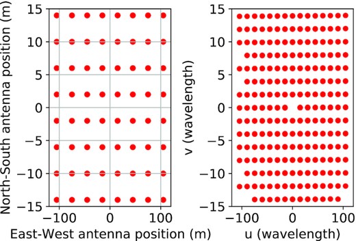
Antenna position (left) and UV coordinate of the PAPER-64 array. The North–South and East–West antenna coordinates are in meter, and the UV coordinates are in wavelengths at 150 MHz (right).
Summary of observational parameters and their values used in this work.
| Parameter | Value |
|---|---|
| PAPER array location | |$\mathrm{30.7^{o} S, 21.4^{o}\, E}$| |
| Observation dates | 2012 November 10 to 2012 November 11 |
| Observing mode | Drift-scan |
| Time resolution | ∼42.9 s |
| Frequency range | 120 MHz–168 MHz |
| Frequency resolution | 0.49 MHz |
| Number of antenna | 61 |
| Field of view | 60○ |
| Visibility polarization | XX, YY |
| Shortest baseline | 4 m |
| Longest baseline | 212 m |
5 RESULTS
5.1 Post-CorrCal spectral structure of data
After CorrCal implementation, we have tried to compare the structure of data as a function of frequency. Fig. 9 depicts the real part of visibility against frequency for a single integration time of a given baseline. The careful examination of the plot shows that the real visibility gets spectrally smoother (red curve) after CorrCal re-calibration. It signifies the reduction of the spectral structure of the visibility measurements after re-calibration. Considering that, in the following section, we present the effect of re-calibration on the delay transformed power spectra (Parsons & Backer 2009).
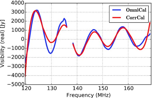
The real part of visibility data (JD2456242.25733) as a function of frequency at a single timestamp for an EW baseline of length about 30 m for both calibrations approaches. Line discontinuity corresponds to the flagged frequency channels. The spectral structure looks slightly reduced after CorrCal (red curve).
5.2 Delay-space power spectra
The statistical analysis of the Fourier mode of the power spectrum (k⊥, k∥) for low-frequency observations is a powerful tool to probe the EoR (Morales & Hewitt 2004). This method shows the existence of distinctive regions dominated by 21-cm signal and foreground contaminants in a 2D line of sight (k∥) and transverse co-moving |$\left(k_{\perp }=\sqrt{k^{2}_{x}+k^{2}_{y}}\right)$| Fourier plane. The spectrally smooth foreground is expected to contaminate the region of low k∥ values, while the vast majority of k∥ values are free from these contaminants (Liu et al. 2014a). Nevertheless, several studies have shown that foreground contamination may go further to the higher k∥ values because of chromatic interaction of interferometry with intrinsically smooth foreground (Morales et al. 2012; Parsons et al. 2012; Vedantham, Shankar & Subrahmanyan 2012; Thyagarajan et al. 2013; Dillon et al. 2014; Liu et al. 2014a; Liu, Parsons & Trott 2014b). This effect leads to the distinctive wedge-like structure in k⊥ and k∥ Fourier space, leaving the foreground-free EoR window beyond the wedge (see results in Figs. 10 and 11 and discussions there).
To convert the measured visibility to 2D power spectrum in k∥ and k⊥ space, the per-baseline delay transform method is used. The technique was first introduced by Parsons & Backer (2009). As thoroughly presented in Parsons et al. (2012), the delay transformed visibility is obtained by inverse Fourier transforming of each baseline along the frequency axis. The method allows the smooth foreground to localize at the central region between the negative and positive geometric delay limits, and any spectrally unsmooth structure such as 21-cm signal may spread across delay axis (Parsons et al. 2012). We will review the mathematical formalism of the per baseline delay-transform method in Appendix A. In our analysis, we use Stokes I visibilities7 taken by PAPER-64 array from Julian date 2456242.17382 to 2456242.65402 (2012 November 10–11) to form the 2D power spectrum using delay transform method, a total of about 9-h observation over frequencies 140–160MHz.
Following Parsons et al. (2012) and Pober et al. (2013), we apply the Blackman–Harris window function during the delay-transform stage to minimize the foreground leakage caused by the finite bandwidth of frequency. This technique allows the EoR window to be mostly dominated by 21-cm brightness temperature by reducing the foreground spectral leakage to the smallest possible amount (Parsons et al. 2012; Pober et al. 2013). We employ the one-dimensional (1D) CLEAN algorithm on the delay-transformed data to reduce the effect introduced by RFI flagging and to increase the resolution in delay space (Pober et al. 2013). We then cross-multiply the consecutive integration time to avoid the noise bias. After these stages, we form the cylindrical delay power spectrum in k space using equation (A5).
Fig. 10 shows the delay power spectra where the positive and negative values of k∥ have not been averaged together. This form of power spectra is expected because emissions from the negative and positive delay directions are proportional to the negative and positive k∥, respectively. The delay power spectra from emissions near-zero delays (where k∥ ∼ 0) are confined within the central region of the 2D delay power spectra. It corresponds to foreground emissions from the peak primary beam response of the instrument.
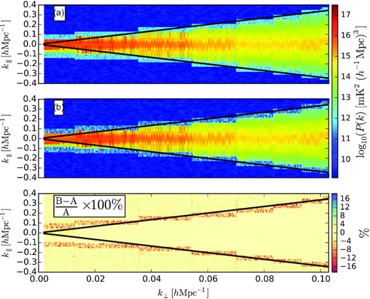
Delay power spectra on either side of k∥ direction. Foreground wedges are confined under the region bounded by the black line or the horizon line. (A) The delay power spectra for data already calibrated with OmniCal. (B) Power spectra after CorrCal re-calibration. The lower panel displays linear scale percentage deviation. The negative percentage deviation in power at the bin right on the horizon shows that the wedge has become tighter after CorrCal re-calibration.
However, from Fig. 10, we see that the strength of power spectra around zero delay decreases as one moves from the lower k⊥ to higher k⊥ regions. Furthermore, for both calibration approaches, more emission goes beyond the horizon limit for shortest baselines (smallest k⊥ values). This effect is because shorter baselines resolve out less of the Galactic synchrotron so that emission will be brighter and sidelobes extend further in k∥ (Pober et al. 2013).
The black diagonal line represents the horizon limit determined by baseline length and the source location relative to the main field of view of the array, marking the boundaries of the foreground wedge. Its analytic expression has been defined in equation (A7). The spectral-smooth emissions are supposed to be confined within that limit, and any emissions that are intrinsically unsmooth with frequency are moving beyond the horizon limit. The calibration error plays a non-negligible role in this regard in imparting the spectral structure to emissions that were originally spectrally smooth as discussed earlier. This unnatural spectral structure, imparted due to calibration error or other effects, will affect the EoR window by scattering power beyond the wedge limits. To see CorrCal’s impact on the delay power spectra, we compare foreground power in a wedge region of the power spectrum, and outside of it in which the 21-cm signal is dominating by taking the percentage deviation between power after CorrCal and OmniCal, shown in the bottom panel of Fig. 10. It is apparent that the power spectra inside and outside the wedge region are comparable for both calibration approaches. However, we observe a consistent drop in power at the bin right on the horizon after CorrCal. Most importantly, this is consistent with some of the analyses done with MWA in (Li et al. 2018; Li et al. 2019; Zhang et al. 2020) that demonstrate redundant calibration’s ability to make small improvements in the modes nearest (but not inside) the wedge. This phenomenon suggests a reduction in the spectral structure of the data after re-calibration with CorrCal.
The well-known wedge-shaped foreground power spectra from our analysis are shown in Fig. 11. We generate this form of power spectra by averaging power from both positive and negative k∥ directions and folding it over the centre of the zero-delay line (where k∥ = 0) of Fig. 10. A similar feature of power spectra has been observed from PAPER-64 data in Pober et al. (2013), as displayed in Fig. 3 of their work. Moreover, Kohn et al. (2016) have reported a wedge-like structure from the analysis of PAPER-32 data. In our analysis, Figs 11(a) and (b), respectively, display the wedge-shaped power spectra to data already calibrated using OmniCal and to data after CorrCal re-calibration. The middle panel in Fig. 11(c) shows power spectra after data have been calibrated using point sources information in CorrCal. For each case, the wedge extends to higher values of k∥ at a longer baseline (k⊥) regime, demonstrating how the theoretical wedge limit increases as a function of baseline length. In addition, sources that are located far away from the pointing centre of the primary beam will also appear at higher delays, corresponding to higher k∥. The relative deviation of power in percent between CorrCal and OmniCal calibration approaches is shown in the third (CorrCal without sky sources information) and fourth (CorrCal with sky sources information) panels of Fig. 11 from left to right, respectively. The negative percentage deviation at the bin right on the horizon in |$\mathrm{[(B-A)/A]\times 100{{\ \rm per\ cent}}}$| and |$\mathrm{[(C-A)/A]\times 100{{\ \rm per\ cent}}}$| of Fig. 11 indicates that the power spectra around the wedge limit have become slightly tighter after CorrCal re-calibration. This effect is not considerably saturated if we include the sources’ information in CorrCal formalism as shown in the right-hand panel of the figure.
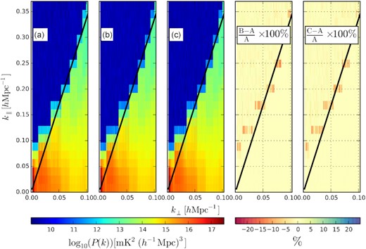
Same as Fig. 10 but averaged and folded over the delay centre to obtain the ‘wedge’-shaped delay power spectra. From left to right: (A) The power spectra generated from data already calibrated with OmniCal package; (B) the power spectra obtained after data have re-calibrated using without source information in CorrCal; (C) power spectra after re-calibration using source information in CorrCal. The right two panels show the linear scale percentage deviation without and with sources information in CorrCal formalism, respectively. The black diagonal line marks the horizon limit (τH).
The R.H.S panel of Fig. 12 depicts a portion of 2D power spectra for a given group of baselines whose lengths are about 150 m. We average over k⊥ axis over the range of |$0.0733\, h\, {\rm Mpc}^{-1} \lt k_{\perp } \lt 0.0736\, h\, {\rm Mpc}^{-1}$| to generate the corresponding 1D power spectra shown on the L.H.S of Fig. 12. From this figure, we observe that there is a steep falloff of the power spectrum right away the horizon limit as expected, showing that the foreground power confined within the slice of the wedge is brighter than the 21-cm signal by 4–5 orders of magnitude. This sharp falloff follows the same trend for both calibration schemes. However, the inclusion of sky sources statistics as a prior during CorrCal re-calibration step does not show the significant change in the power spectra, as shown on the L.H.S of Fig. 12.
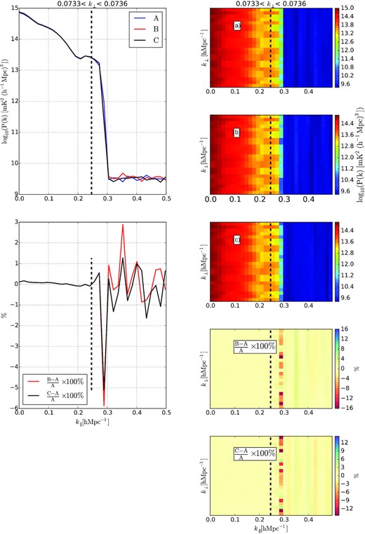
Right: Two-dimensional power spectra after (A) OmniCal, (B) CorrCal re-calibration without sources info, and (C) CorrCal re-calibration with sources information. The lower panels are the percentage deviation of B to A and C to A, respectively. The black dashed vertical line is representing the horizon (τH) limit. Left: The averaged slice of power spectra from |$k_{\perp }=0.0733~h\, {\rm Mpc}^{-1}$| to |$k_{\perp }=0.0736~h\, {\rm Mpc}^{-1}$| to both calibration schemes. The top panel is the one-dimensional average power spectrum as a function of k∥ for a portion of baselines (|$\sim 150\rm m$|) to both calibration strategies. The bottom panel is the percentage deviation.
6 CONCLUSIONS
In this work, we used a new calibration scheme (CorrCal) to re-calibrate the PAPER64 observations. Our new calibration scheme boils down to the covariance-based calculation of χ2, allowing one to include the relaxed array redundancy and sky information into its formalism. This formalism also provides space for cross-frequency bandpass calibration. Furthermore, the inclusion of known sources information in CorrCal breaks the statistical isotropy of the sky, which sets the overall phase gradient degenerate parameter across the array. We have compared the spectral smoothness of the observed data before and after CorrCal’s application. We observed that the spectral structure of the visibility data after CorrCal becomes slightly reduced, for instance, as shown in Fig. 9. The significant factor for this improvement could be the CorrCal natural formalism to carry out the cross-frequency bandpass calibration.
We implemented the delay-transform method (Parsons & Backer 2009; Parsons et al. 2012) to filter out smooth foregrounds from the spectrally structured weak 21-cm signal in 2D Fourier k −space. The comparison results in the delay space show that the power spectra around the foreground wedge limit have been reduced by about |$6{{\ \rm per\ cent}}$| after the CorrCal re-calibration. Nevertheless, this effect does not significantly improve the power spectrum in any bin around the horizon limit of the foreground wedge and further investigation will be needed to test the algorithm effectiveness and its implementation methods. The current numerical tests lay the foundation of calibration radio instruments using correlated signals on the sky. Our future work will include possible beam shape errors, antenna pointing errors, and position errors, and improve the CorrCal method by using sky and antenna simulation (e.g. pyuvsim) and compare it with sky-based calibration and redundant baseline calibration. In conclusion, the CorrCal may be an alternative calibration method for radio interferometry, which potentially helps to probe the EoR using the 21-cm signal.
ACKNOWLEDGEMENTS
We would like to acknowledge the PAPER collaboration for providing us data that have been used in this work. YZM acknowledges the support of NRF-120385, NRF-120378, and NSFC-11828301. PK acknowledges funding support from the South African–China Collaboration program in Astronomy at the University of KwaZulu-Natal.
DATA AVAILABILITY
The data underlying this article will be shared on reasonable request to the corresponding author.
Footnotes
The prototype version of the software located on https://github.com/sievers/corrcal2.git is being used for this work.
It is worth noticing that Liu et al. (2010) investigated the Taylor expansion of the sky to deal with direction dependence or non-redundancy.
Note that these are not true Stokes I would rather the average of XX and YY visibilities (see Section A).
REFERENCES
APPENDIX A: DELAY SPECTRUM
APPENDIX B: DETERMINING THE EOR SIGNAL LOSS IN CorrCal ANALYSIS
To determine whether our analysis methods are lossless or not in the EoR power spectrum estimate, first, we simulate visibility data using HERA simulation pipeline (hera_sim8). For this simulation, we use the analytic airy beam model (the same for all antenna elements), the simulated antenna gains, the GaLactic and Extragalactic All-sky MWA (GLEAM) sky sources (Hurley-Walker et al. 2017), and the simulated EoR signal using hera_sim. Then, to quantify our new calibration approach does not lead to the EoR power spectrum signal suppression, we propagate simulated data into the CorrCal for calibration. We then compute the 2D power spectrum for both simulated and recovered data after CorrCal calibration using the delay spectrum approach described in Appendix A. Fig. B1 shows the delay space power spectra for both simulated and recovered data. From the figure, it is apparent that the recovered power spectra after CorrCal are comparable to the expected one, confirming that CorrCal calibration method does not lead to significant signal loss.
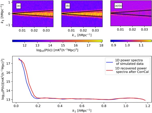
Top: (A) Expected delay power spectra, (B) recovered power spectra after CorrCal calibration, and (C) the power spectra ratio of B to A. The solid black dashed line is the horizon limit, τH. Bottom: Averaged 1D power spectra as a function of k∥ for a portion of baselines in the |$\sim 30~\rm m$| group.
