


ABSTRACT
Gaps imaged in protoplanetary discs are suspected to be opened by planets. We compute the present-day mass accretion rates |$\dot{M}_{\rm p}$| of seven hypothesized gap-embedded planets, plus the two confirmed planets in the PDS 70 disc. The accretion rates are based on disc gas surface densities Σgas from C18O observations, and planet masses Mp from simulations fitted to observed gaps. Assuming accretion is Bondi-like, we find in eight out of nine cases that |$\dot{M}_{\rm p}$| is consistent with the time-averaged value given by the current planet mass and system age, Mp/tage. As system ages are comparable to circumstellar disc lifetimes, these gap-opening planets may be undergoing their last mass doublings, reaching final masses of |$M_{\rm p} \sim 10\rm{\!-\!}10^2 \, M_\oplus$| for the non-PDS 70 planets, and |$M_{\rm p} \sim 1\!-\!10 \, M_{\rm J}$| for the PDS 70 planets. For another 15 gaps without C18O data, we predict Σgas by assuming their planets are accreting at their time-averaged |$\dot{M}_{\rm p}$|. Bondi accretion rates for PDS 70b and c are orders of magnitude higher than accretion rates implied by measured U-band and H α fluxes, suggesting most of the accretion shock luminosity emerges in as yet unobserved wavebands, or that the planets are surrounded by dusty, highly extincting, quasi-spherical circumplanetary envelopes. Thermal emission from such envelopes or from circumplanetary discs, on Hill sphere scales, peaks at wavelengths in the mid-to-far-infrared and can reproduce observed mm-wave excesses.
1 INTRODUCTION
The Atacama Large Millimeter Array (ALMA) has revealed gaseous protoplanetary discs to be ringed and gapped, with HL Tau (ALMA Partnership et al. 2015) and discs from the DSHARP (Andrews et al. 2018) and MAPS (Oberg et al. 2021) surveys providing stunning examples (see also Cieza et al. 2019; Andrews 2020). The annular structures observed at orbital distances of r ∼ 10–100 au are commonly interpreted as being carved by protoplanets within the gaps, by analogy with shepherd satellites opening gaps in planetary rings (e.g. Goldreich & Tremaine 1979). A few dozen candidate planets have been so hypothesized with masses Mp of several Earth masses M⊕ to a few Jupiter masses MJ (Zhang et al. 2018; fig. 1 of Lodato et al. 2019; and Table 1 of this paper).
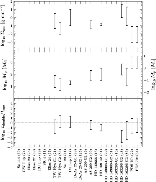
Top panel: Gas surface density Σgas at the centres of gaps hypothesized (confirmed for PDS 70) to host planets, for the subset of systems detected in C18O. System names on the horizontal axis are followed by ‘G#’ to identify a specific gap in systems with multiple gaps, and by the planet’s orbital radius r in units of au in parentheses. Systems are listed in order of increasing host stellar mass M⋆, except for PDS 70 which as the only transitional disc in our sample is placed at the end. For TW Hya, we estimate Σgas from the C18O line flux (Nomura et al. 2021), while for AS 209, IM Lup, HD 169142, and HD 163296 Σgas derives from detailed thermo-chemical modelling (Isella et al. 2016; Fedele et al. 2017; Favre et al. 2019; Zhang et al. 2021). For PDS 70, we bound Σgas using the C18O 2-1 flux outside the disc cavity and the 12CO 3-2 flux inside the cavity (Facchini et al. 2021). Middle panel: Planet masses Mp. For the non-PDS 70 planets Mp is drawn from gap-fitting simulations by Zhang et al. (2018) and Dong & Fung (2017) scaled to viscosities α = 10−5–10−3. For PDS 70b and c, |$M_{\rm p} = 1\rm{\!-\!}10\, M_{\rm J}$| roughly encompasses values from cooling models (e.g. Haffert et al. 2019). Bottom panel: Mass doubling times |$t_{\rm double} \equiv M_{\rm p}/\dot{M}_{\rm p}$| calculated assuming accretion at the Bondi rate (equation 3). Accretion rates |$\dot{M}_{\rm p}$| are evaluated using Σgas and Mp as above, plus h and r compiled in Table 1. Error bars account for uncertainties in Σgas and Mp, with tdouble ∝ 1/(MpΣgas). Eight of the nine hypothesized planets may have tdouble comparable to their system age tage, a plausible result that if true suggests these planets are undergoing their last doublings.
Properties of gapped discs and the planets hypothesized to reside within them (confirmed in the case of PDS 70). Column headings: (1) System name. For systems with multiple gaps, we append ‘G#’ to distinguish between different gaps. (2) Stellar mass (Blondel & Djie 2006; Ducourant et al. 2014; Andrews et al. 2018; Keppler et al. 2019; Oberg et al. 2021) (3) Stellar age (Ducourant et al. 2014; Pohl et al. 2017; Andrews et al. 2018; Müller et al. 2018) (4) Planet orbital radius (Dong & Fung 2017; Keppler et al. 2018; Zhang et al. 2018) (5) Planet mass. For the non-PDS 70 planets (first 22 entries), the quoted range in Mp corresponds to disc viscosities α = 10−5–10−3, scaled from the gap-fitting, two-fluid, planet–disc simulations of Zhang et al. (2018) and Dong & Fung (2017) (see Section 2.4.1). The ranges on Mp for PDS 70b and c roughly cover values inferred from infrared photometry and cooling models (Keppler et al. 2018; Müller et al. 2018; Wang et al. 2020). (6) Gas surface density at the planet’s location, as inferred from C18O emission (Isella et al. 2016; Fedele et al. 2017; Favre et al. 2019; Facchini et al. 2021; Nomura et al. 2021; Zhang et al. 2021). The quoted ranges on Σgas in AS 209, IM Lup, HD 163296, and TW Hya accommodate the possibility that the CO:H2 abundance ratio in these discs is lower than in the ISM (Zhang et al. 2019; Calahan et al. 2021; Zhang et al. 2021). (7) Dust surface density at the planet’s location (Fedele et al. 2017; Huang et al. 2018; Benisty et al. 2021; Nomura et al. 2021) accounting for an assumed factor of 7 uncertainty in opacity. Because most gaps are only marginally resolved in mm continuum emission we are likely overestimating Σdust (see Section 2.2). Daggers (†) mark the five gaps which Jennings et al. (2021) found to have lower dust continuum intensities and hence lower Σdust than Huang et al. (2018) found. (8) Disc aspect ratio, mostly taken from Zhang et al. (2018) except for those marked with an asterisk (see Section 2.3). The values for tage, Mp, Σgas, Σdust, and h/r are uncertain and quoted to only one significant figure.
| (1) | (2) | (3) | (4) | (5) | (6) | (7) | (8) |
|---|---|---|---|---|---|---|---|
| Name | M⋆ (M⊙) | tage (Myr) | r (au) | Mp (M⊕) | Σgas (g cm−2) | Σdust (g cm−2) | h/r |
| Sz 114 | 0.17 | 1 | 39 | 3–6 | N/A | 0.08–0.6 | 0.1 |
| GW Lup | 0.46 | 2 | 74 | 2–10 | N/A | 0.03–0.2† | 0.08 |
| Elias 20 | 0.48 | ≤ 0.8 | 25 | 8–20 | N/A | 0.1–0.7 | 0.08 |
| Elias 27 | 0.49 | 0.8 | 69 | 3–20 | N/A | 0.05–0.3 | 0.09 |
| RU Lup | 0.63 | 0.5 | 29 | 10–20 | N/A | 0.2–1 | 0.07 |
| SR 4 | 0.68 | 0.8 | 11 | 60–700 | N/A | 0.03–0.2† | 0.05 |
| Elias 24 | 0.78 | 0.2 | 57 | 30–300 | N/A | 0.003–0.02 | 0.09 |
| TW Hya-G1 | 0.80 | 8 | 21 | 8–80 | 0.04–3 | 0.06–0.4 | 0.08* |
| TW Hya-G2 | 0.80 | 8 | 85 | 5–50 | 0.008–0.2 | 0.002–0.02 | 0.09* |
| Sz 129 | 0.83 | 4 | 41 | 5–10 | N/A | 0.2–1 | 0.06 |
| DoAr 25-G1 | 0.95 | 2 | 98 | 20–30 | N/A | 0.05–0.3 | 0.07 |
| DoAr 25-G2 | 0.95 | 2 | 125 | 5–10 | N/A | 0.08–0.6 | 0.07 |
| IM Lup | 1.1 | 0.5 | 117 | 10–30 | 0.1–10 | 0.03–0.2 | 0.1* |
| AS 209-G1 | 1.2 | 1 | 9 | 60–700 | N/A | 0.05–0.3† | 0.04 |
| AS 209-G2 | 1.2 | 1 | 99 | 30–200 | 0.04–0.4 | 0.008–0.06 | 0.06* |
| HD 142666 | 1.58 | 10 | 16 | 10–100 | N/A | 0.2–1 | 0.05 |
| HD 169142 | 1.65 | 10 | 51 | 30–300 | 0.1–0.2 | ≤0.01 | 0.07* |
| HD 143006-G1 | 1.78 | 4 | 22 | 400–6000 | N/A | 0.003–0.02† | 0.04 |
| HD 143006-G2 | 1.78 | 4 | 51 | 20–100 | N/A | 0.02–0.2 | 0.05 |
| HD 163296-G1 | 2.0 | 10 | 10 | 30–200 | N/A | 0.2–1 | 0.07* |
| HD 163296-G2 | 2.0 | 10 | 48 | 90–700 | 1–40 | 0.003–0.02† | 0.08* |
| HD 163296-G3 | 2.0 | 10 | 86 | 10–300 | 0.1–20 | 0.01–0.09 | 0.08* |
| PDS 70b | 0.88 | 5 | 22 | 300–3000 | 0.0008–0.08 | ≤0.02 | 0.07* |
| PDS 70c | 0.88 | 5 | 34 | 300–3000 | 0.0008–0.08 | ≤0.02 | 0.08* |
So far disc-embedded protoplanets have been directly imaged in one system: PDS 70b and c are confirmed in the near-infrared to orbit at r ∼ 20–40 au within the central clearing of the system’s transitional disc (Keppler et al. 2018; Haffert et al. 2019; Wang et al. 2020, 2021, and references therein). These protoplanets, each estimated to be of order a Jupiter mass, have been imaged at multiple wavelengths, from the ultraviolet at 336 nm (Zhou et al. 2021) to Hα (Haffert et al. 2019) to the sub-millimetre continuum (Isella et al. 2019; Benisty et al. 2021). Aside from PDS 70b and c, all other planets proposed to explain disc substructures remain undetected. There are unconfirmed near-infrared point sources in HD 163296 (Guidi et al. 2018) and Elias 24 (Jorquera et al. 2021), and kinematical evidence for planetary perturbations to the rotation curve in HD 163296 (Teague et al. 2018, 2021).
Are the disc gaps and rings imaged by ALMA and in the infrared (e.g. Asensio-Torres et al. 2021) really caused by planets? What can we hope to learn from DSHARP discs and similar systems about how planets form? At the top of the list of measurables should be the planetary mass accretion rate |$\dot{M}_{\rm p}$| and how it depends on Mp and ambient disc properties like density and temperature. The planet masses inferred from modelling disc substructures are frequently dozens of Earth masses (e.g. Dong & Fung 2017; Zhang et al. 2018; our Table 1),1 large enough that an order-unity fraction of their mass should be in the form of accreted hydrogen. For such planets with self-gravitating gas envelopes, accretion may be hydrodynamic, i.e. regulated by how much mass the surrounding nebula can deliver to the planet through transonic/supersonic flows (e.g. D’Angelo, Kley & Henning 2003; Machida et al. 2010; Tanigawa & Tanaka 2016; Ginzburg & Chiang 2019a). This phase is distinct from an earlier thermodynamic phase of gas accretion limited by the rate at which the nascent envelope can cool and contract quasi-hydrostatically (e.g. Lee & Chiang 2015; Ginzburg, Schlichting & Sari 2016; Chachan, Lee & Knutson 2021). Are the inferences of planets still immersed in their parent discs consistent with our ideas of hydrodynamic accretion? To what final masses should we expect the hypothesized planets to grow?
This paper takes stock of the developing landscape of disc substructures and directly imaged protoplanets to address these and other questions. Our goal is to assess what we have learned (if anything) about planet formation from the multiwavelength observations, and how theory fares against data. In these early days, the analysis is necessarily at the order-of-magnitude level. We begin in Section 2 by documenting our sources (mostly DSHARP) for disc and putative planet properties. These quantities are used in Section 3 to estimate the present-day |$\dot{M}_{\rm p}$| according to theory and to evaluate whether the corresponding planet growth time-scales |$M_{\rm p}/\dot{M}_{\rm p}$| make sense in comparison to the system ages. The mass accretion rates are also used to evaluate accretion luminosities, and we discuss how accretion may be playing out in the circumplanetary environments of PDS 70b and c. In Section 4, we summarize and offer an outlook.
2 OBSERVATIONAL DATA
Table 1 compiles disc and candidate planet properties taken directly from the literature or derived therefrom. Quantities of interest include the host stellar mass M⋆ and planet mass Mp, the gas and dust surface densities Σgas and Σdust at planet orbital distance r, and the local disc aspect ratio h/r. To the 19 DSHARP protoplanets modelled by Zhang et al. (2018) we add the one candidate protoplanet in HD 169142 (Dong & Fung 2017), the two candidates in TW Hya (Dong & Fung 2017), and the two confirmed planets in PDS 70 (Keppler et al. 2018; Haffert et al. 2019).
2.1 Gas surface densities Σgas
We focus on systems for which emission from optically thin C18O has been spatially resolved. More abundant isotopologues of CO are usually optically thick (including 13CO; van der Marel et al. 2015; Favre et al. 2019) and as such yield only lower limits on Σgas. Hydrogen surface densities derived from C18O emission are none the less uncertain. The gas-phase CO:H2 abundance ratio XCO is hard to determine; it may be lower in protoplanetary discs than in the interstellar medium (ISM) because of condensation of CO on to dust grains or chemistry driven by cosmic rays (e.g. Schwarz et al. 2018). We will try to account for the possibility of gas-phase CO depletion in what follows. Surface densities at the centres of gaps where planets supposedly reside may also be overestimated if gaps are spatially underresolved, with emission from gap edges contaminating the emission at gap centre. Such contamination might not be too serious for the gaps considered in this subsection, whose radial widths are larger (marginally) than the corresponding ALMA beams. Also, simulations predict gas density variations less than a factor of 10 across gaps for |$M_{\rm p} \lesssim 60 \, M_\oplus$| (e.g. Dong et al. 2017, top left panel of their fig. 8).
Of the twenty-four planets in our sample we have measurements of Σgas based on C18O emission (in conjunction with other emission lines) for nine planets in six systems.
2.1.1 Gas surface density: AS 209
The protoplanetary disc around AS 209 has five annular gaps in dust continuum emission at orbital radii |$r \approx 9,\, 24,\, 35,\, 61,$| and 99 au (Guzmán et al. 2018; Huang et al. 2018). Zhang et al. (2018) demonstrated that the four gaps from 24–99 au can be produced by a single planet situated within the outermost gap at 99 au (see their fig. 19). Favre et al. (2019) and Zhang et al. (2021) observed a broad gap in C18O (2-1) emission extending from ∼60 to 100 au. Favre et al. (2019) modelled the emission using the DALI thermo-chemical code (Bruderer 2013) and took the gas density profile to include two gaps coincident with the dust gaps at 61 and 99 au. They showed these two gas gaps could be smeared by the ALMA beam into a single wide gap like that observed in molecular emission. At the bottom of the 99 au gap where the planet is believed to reside, they fitted |$\Sigma _{\rm gas}\approx 0.04\rm{\!-\!}0.08\, \rm g\, cm^{-2}$| (see the blue and green curves in their fig. 6).
Zhang et al. (2021) modelled the C18O emission using the thermo-chemical code RAC2D (Du & Bergin 2014), including only a single gap. They initialized their models with an ISM-like XCO which decreased from CO freeze-out and chemistry over the simulation duration of 1 Myr. They found |$\Sigma _{\rm gas}\approx 0.08 \, \rm g\, cm^{-2}$| at 99 au (their fig. 16), similar to Favre et al. (2019). Zhang et al. (2021) also considered the possibility that there is no gap in H2 and that the observed gap in C18O is due to XCO being somehow locally depleted beyond the predictions of RAC2D. Assuming a total gas-to-dust ratio of 10 by mass (their table 2), they estimated in this super-depleted XCO scenario |$\Sigma _{\rm gas}\approx 0.4 \, \rm g\, cm^{-2}$| at 99 au (their fig. 5; see also Alarcón et al. 2021 who advocated on separate grounds for a depleted CO:H2 ratio in AS 209).
We combine the results of Favre et al. (2019) and Zhang et al. (2021) to consider |$\Sigma _{\rm gas}= 0.04\rm{\!-\!}0.4 \, \rm g\, cm^{-2}$| for the gap AS 209-G2 at r = 99 au (Table 1).
2.1.2 Gas surface density: HD 163296
Dust continuum observations of HD 163296 reveal gaps centred at 10, 48, and 86 au (Isella et al. 2016; Huang et al. 2018), each opened by a separate planet according to Zhang et al. (2018). Isella et al. (2016) fitted the emission at r ≳ 25 au from three CO isotopologues assuming an ISM-like value of XCO and found |$\Sigma _{\rm gas}\approx 2.5\rm{\!-\!}10\, \rm g\, cm^{-2}$| at 48 au and |$\Sigma _{\rm gas}\approx 0.1\rm{\!-\!}2 \, \rm g\, cm^{-2}$| at 86 au (their fig. 2, blue curve; note the gap radii in their figure are about 20 per cent larger than the values we use because they used a pre-GAIA source distance). The thermo-chemical models of Zhang et al. (2021) predict roughly consistent values of |$\Sigma _{\rm gas}\approx 1 \, \rm g\, cm^{-2}$| and |$\Sigma _{\rm gas}\approx 0.6 \, \rm g\, cm^{-2}$| respectively (see their fig. 16). If instead the CO:H2 abundance is much lower than predicted by their models and the gas-to-dust ratio is 60 (their table 2), then |$\Sigma _{\rm gas}\approx 40\, \rm g\, cm^{-2}$| and |$\Sigma _{\rm gas}\approx \, 20\, \rm g\, cm^{-2}$| (their fig. 5).
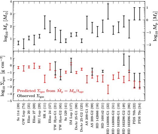
Top panel: Same as the middle panel of Fig. 1, with Mp now plotted for all 24 planets in our sample. Bottom panel: Same as the top panel of Fig. 1, with red points added to mark Σgas predicted from equation (5). The prediction assumes that each planet is accreting at the Bondi-like rate given by (3) and that |$\dot{M}_{\rm p} = M_{\rm p}/t_{\rm age}$| (equivalently tdouble = tage; for Elias 24 we use the upper limit on tage). The last equality is motivated by the bottom panel of Fig. 1. The evaluation of (5) uses Mp in the top panel plus r and h listed in Table 1. Red error bars reflect the range of Mp values considered.
The above estimates of Σgas are combined to yield the full ranges quoted in Table 1, |$\Sigma _{\rm gas}= 1\rm{\!-\!}40\, \rm g\, cm^{-2}$| for HD 163296-G2 at 48 au, and |$\Sigma _{\rm gas}= 0.1\rm{\!-\!}20\, \rm g\, cm^{-2}$| for HD 163296-G3 at 86 au.
2.1.3 Gas surface density: IM Lup
IM Lup presents a shallow gap at r ≈ 117 au in millimetre continuum images (Huang et al. 2018) which Zhang et al. (2018) attributed to a 10–30 M⊕ planet. Zhang et al. (2021) found |$\Sigma _{\rm gas}\approx 0.1 \, \rm g\, cm^{-2}$| in their RAC2D modelling which includes CO freeze-out and chemistry (their fig. 16). Alternatively, for a super-depleted CO:H2 scenario and gas-to-dust ratio of 100 (their table 2), |$\Sigma _{\rm gas}\approx 10\, \rm g\, cm^{-2}$| (their fig. 5). We allow for both possibilities and take |$\Sigma _{\rm gas}= 0.1\rm{\!-\!}10\, \rm g\, cm^{-2}$|.
2.1.4 Gas surface density: HD 169142
HD 169142 features an annular gap at 50 au in near-infrared scattered light (Quanz et al. 2013) and mm-wave continuum emission (Fedele et al. 2017). In C18O emission, Fedele et al. (2017) found evidence for a cavity inside r ≈ 50 au and used DALI to infer |$\Sigma _{\rm gas}\approx 0.1\rm{\!-\!}0.2\, \rm g\, cm^{-2}$| near the cavity outer edge (their fig. 5, top left panel, blue curve). Mid-plane gas temperatures according to the same thermo-chemical model (fig. 5, bottom centre panel) are ∼30–40 K, higher than the CO freeze-out temperature of ∼20 K. CO may still be depleted for other reasons (Schwarz et al. 2018) but without a model we cannot quantify the uncertainty.
2.1.5 Gas surface density: TW Hya
Near-infrared scattered light images reveal annular gaps at r ≈ 21 au (TW Hya-G1) and 85 au (TW Hya-G2) (van Boekel et al. 2017). The inner gap may also have been detected in the mm continuum by Andrews et al. (2016), albeit slightly outside the gap in scattered light (their fig. 2). Nomura et al. (2021) studied TW Hya in the J = 3 − 2 transition of C18O. Near the inner gap they measured a wavelength-integrated line flux of 5 mJy beam−1 km s−1 (their fig. 2, middle panel, orange curve). We extrapolate their radial intensity profile, which cuts off at 80 au, to the outer gap at 85 au and estimate there a flux of 1 mJy beam−1 km s−1. Using temperatures of 60 and 20 K for the inner and outer gaps respectively (Section 2.3.3), we convert these fluxes to C18O column densities (e.g. Mangum & Shirley 2015, their equation B2). Then assuming XCO = 10−4 and a 18O: 16O gas-phase abundance ratio of 2 × 10⁻³ (e.g. Qi et al. 2011), we calculate |$\Sigma _{\rm gas}= 0.04\, \rm g\, cm^{-2}$| and |$0.008\, \rm g\, cm^{-2}$| for the two gaps. These surface densities could be underestimated by factors of 70 and 30 (assuming a gas-to-dust ratio of 100), respectively, if CO is somehow super-depleted (Zhang et al. 2019, their fig. 8, second panel, blue curve). Thus we have |$\Sigma _{\rm gas}\approx 0.04\rm{\!-\!}2.8\, \rm g\, cm^{-2}$| for TW Hya-G1 and |$\Sigma _{\rm gas}\approx 0.008\rm{\!-\!}0.24\, \rm g\, cm^{-2}$| for TW Hya-G2.
2.1.6 Gas surface density: PDS 70
Facchini et al. (2021) studied PDS 70 in the J = 2 − 1 transition of |$\rm C^{18}O$|, but the beam size at this wavelength was too large to resolve the cavity within which the two planets reside. We therefore resort to using the C18O emission just outside the cavity to place an upper limit on the gas surface density near the planets. Following the same procedure as for TW Hya, we convert the observed C18O flux outside the cavity into an H2 surface density. We use 30 K as the gas excitation temperature at 80 au, close to the H2CO excitation temperature measured by Facchini et al. (2021, their fig. 7). The gas surface density so derived is |$\Sigma _{\rm gas}= 8 \times 10^{-2}\, \rm g\, cm^{-2}$|. We pair this upper limit with a lower limit derived from optically thick 12CO in the J = 3 − 2 transition. The smaller beam associated with the higher frequency of this transition allowed the cavity to be resolved by Facchini et al. (2021). Near the positions of the planets at r ∼ 22 − 34 au, the observed 12CO line flux is 37 K km s−1, which for an assumed temperature of T ∼ 60 K (scaled from 30 K at 80 au using T ∝ r−3/7 for a passively irradiated disc; Chiang & Goldreich 1997) yields a lower bound on Σgas of |$8\times 10^{-4}\, \rm g\, cm^{-2}$|. The temperatures quoted above are high enough to avoid CO freeze-out, though we cannot rule out that gas-phase CO is depleted from other effects (Schwarz et al. 2018).
2.2 Dust surface densities Σdust
Surface densities may be overestimated inside gaps that are spatially underresolved. This may be a much more serious problem for Σdust than for Σgas (cf. Section 2.1) because simulations predict dust surface densities to vary by orders of magnitude across gaps carved by |$M_{\rm p} \gtrsim 10 \, M_\oplus$| planets, with dust gradients steepened by aerodynamic drag (e.g. fig. 1 of Paardekooper & Mellema 2004; fig. 8 of Dong et al. 2017; fig. 4 of Binkert, Szulágyi & Birnstiel 2021). We caution that the values of Σdust we derive may therefore be grossly overestimated. See also Jennings et al. (2021), whose work we describe below.
2.2.1 Dust surface density: DSHARP systems
For all 19 of the DSHARP planets, we estimate Σdust at gap centre using equation (1) and the optical depth profiles in fig. 6 of Huang et al. (2018).
Three of the DSHARP gaps, AS 209-G2 (r = 99 au), Elias 24 (57 au), and HD 143006-G1 (22 au), have bottoms that fall below the 2σ noise floor at τ = 10−2, although apparently only marginally so. For Elias 24 and HD 143006-G1, we set τ = 10−2. For AS 209-G2, while portions of the gap lie below the noise floor, at gap centre there is actually a local maximum (ring) of emission that rises above the noise. We use the peak optical depth of this ring, τ ≈ 2 × 10⁻², to evaluate Σdust. The ‘W’-shaped gap profile for AS 209-G2 resembles transient structures found in two-fluid simulations of low-mass planets embedded in low-viscosity discs (Dong et al. 2017; Zhang et al. 2018).
In their re-analysis at higher spatial resolution of the DSHARP data, Jennings et al. (2021, their fig. 12) found evidence for deeper dust gaps than originally measured by Huang et al. (2018) for GW Lup, HD 163296-G2, SR 4, AS 209-G1, and HD 143006-G1. The reanalysed gaps in the mm continuum are deeper by at least a factor of 10 and in most cases much more. We make a note of these sources in Table 1, but continue to use the Huang et al. (2018) results to compute Σdust for consistency with the rest of our analysis.
2.2.2 Dust surface density: TW Hya
For TW Hya-G1 at 21 au we calculate |$\Sigma _{\rm dust}= 0.06\rm{\!-\!}0.4\, \rm g\, cm^{-2}$| using equations (1)–(2) with Iν = 10 mJy beam−1 (fig. 2, middle panel, purple curve of Nomura et al. 2021) and T = 60 K (Section 2.3.3). For TW Hya-G2 at 85 au we estimate |$\Sigma _{\rm dust}= 0.002\rm{\!-\!}0.02\, \rm g\, cm^{-2}$| using |$I_{\nu } \sim 10^{-1}\,$| mJy beam−1 (this is an extrapolation of the intensity profile measured by Nomura et al. 2021 which does not extend beyond ∼70 au) and T = 20 K. Our estimates of Σdust are consistent with those plotted in fig. 3 of Nomura et al. (2021).
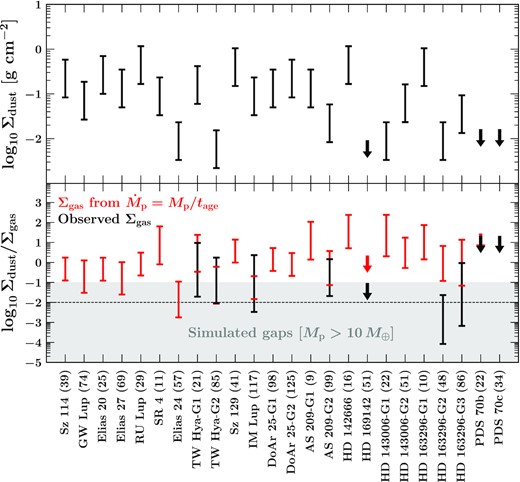
Top panel: Same as the top panel of Fig. 1 but plotting dust surface densities Σdust inside gaps based on observed mm continuum intensities (Huang et al. 2018), assuming the dust is optically thin. Error bars account for a factor of seven uncertainty in the grain opacity but do not account for the limited spatial resolution of the observations which may lead to Σdust being overestimated. For HD 169142 and PDS 70, we plot upper limits on Σdust set by the noise floor of the observations (Fedele et al. 2017; Benisty et al. 2021). Bottom panel: Gap dust-to-gas ratios Σdust/Σgas. In black we combine the values of Σdust with Σgas inferred from C18O intensity maps (Fig. 1, top panel). In red we use the same Σdust data but take Σgas from equation (5), which presumes that planets accrete in a Bondi-like way with growth timescales |$M_{\rm p}/\dot{M}_{\rm p}$| equal to system ages (Fig. 2, red points). The shaded bar covers the range of dust-to-gas ratios found inside gaps opened by planets with Mp > 10M⊕ in two-fluid simulations by Dong et al. (2017). Many of the empirical data lie outside the simulated range, possibly because dust gaps are still underresolved by ALMA and therefore Σdust is overestimated. In support of this idea, Jennings et al. (2021) reanalysed the DSHARP data and found deeper bottoms to the dust gaps in GW Lup, SR 4, AS 209-G1, HD 143006-G1, and HD 163296-G2.
2.2.3 Dust surface density: HD 169142 and PDS 70
For the gap in HD 169142 and central clearing in PDS 70, the continuum emission falls below the 3σ noise floor of the observations (0.21 and 0.0264 mJy beam−1, respectively; Fedele et al. 2017; Benisty et al. 2021). For assumed temperatures of T = 40 K in HD 169142 and T = 60 K in PDS 70, the corresponding upper limits on the dust column are |$\Sigma _{\rm dust}\le 10^{-2}\, \rm g\, cm^{-2}$| and |$\Sigma _{\rm dust}\le 2 \times 10^{-2}\, \rm g\, cm^{-2}$|, respectively.
2.3 Disc scale height h
2.3.1 Disc scale height: DSHARP systems
For most of the DSHARP sample, we adopt the h/r estimates listed in table 3 of Zhang et al. (2018), computed assuming a passive disc irradiated by its host star. For AS 209-G2, all three gaps in HD 163296, and IM Lup, we use more sophisticated estimates of h/r from table 2 of Zhang et al. (2021). In AS 209, Zhang et al. (2021) used the observed 13CO emission surface to fit for |$h/r = 0.06(r/100\, \rm au)^{0.25}$| (since their CO isotopologue data do not extend down to AS 209-G1 at 9 au, we only apply this scale height relation to AS 209-G2 at 99 au). Note that Zhang et al. (2018) found a similar value, h/r = 0.05 at 99 au, reproduced the multigap structure of AS 209. For HD 163296 and IM Lup, Zhang et al. (2021) obtained excellent fits to the spectral energy distributions (their fig. 4) using |$h/r = 0.084(r/100\, \rm au)^{0.08}$| and |$h/r = 0.1(r/100\, \rm au)^{0.17}$|, respectively.3
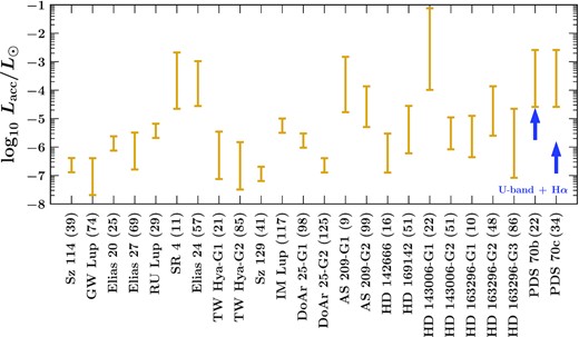
Predicted bolometric accretion luminosities |$L_{\rm acc} = GM_{\rm p}\dot{M}_{\rm p}/R_{\rm p}$| assuming each planet is accreting at the average rate given by its mass and system age |$\dot{M}_{\rm p} = M_{\rm p}/t_{\rm age}$| (equivalently tdouble = tage). For the non-PDS 70 planets we estimate Rp = RJ(Mp/MJ)1/3 for Mp < MJ and Rp = RJ(Mp/MJ)−1/3 for Mp > MJ. For PDS 70b and c we use |$R_{\rm p} = 2\, R_{\rm J}$| following blackbody fits by Wang et al. (2020) to near-infrared photometry. Error bars reflect the adopted range of Mp (see Table 1 or the top panel of Fig. 2), including the dependence of Rp on Mp. The blue arrows show estimates of Lacc for the PDS 70 planets derived from observed U-band (336 nm) and H α fluxes. These values are hard lower limits because the accretion fluxes may be attenuated by dust along the line of sight, or the accretion luminosity may be concentrated in wavebands other than those observed. Figs 5 and 6 showing the SEDs for PDS 70b and c suggest much of the accretion power ultimately emerges in the infrared.
2.3.2 Disc scale height: HD 169142
Fedele et al. (2017) simultaneously fitted the surface density and temperature profiles in HD 169142. We use their aspect ratio of h/r = 0.07 at the gap position; this is similar to the value of h/r = 0.08 found by Dong & Fung (2017) in fitting the gap width to their planet-disk simulations. The aspect ratio relates to the disc mid-plane temperature following h/r = cs/(Ωr) where |$c_s = \sqrt{kT/\mu m_{\rm p}}$| is the sound speed, μ = 2.4 is the mean molecular weight, k is Boltzmann’s constant, mp is the proton mass, |$\Omega = \sqrt{GM_{\star }/r^3}$| is the Keplerian orbital frequency, and G is the gravitational constant. The implied temperature at the gap position is 40 K.
2.3.3 Disc scale height: TW Hya
Calahan et al. (2021) obtained a good fit to the spectral energy of TW Hya using |$h/r = 0.11 \, (r/400\, \rm au)^{0.1}$| (their fig. 5). From this scaling we calculate h/r = 0.08 and h/r = 0.09 at the inner (r = 21 au) and outer (r = 85 au) gap positions, respectively. These aspect ratios correspond to temperatures of 58 and 20 K.
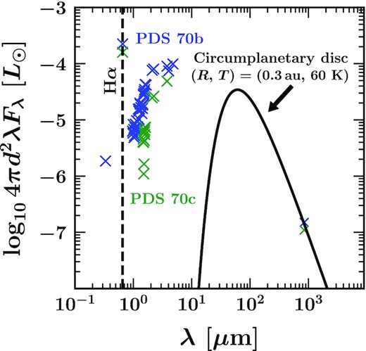
Observed SEDs of the PDS 70 planets (crosses) and emission from a single-temperature blackbody modelling a circumplanetary disc (CPD, black curve). Wavelength is denoted by λ, flux density by Fλ (units of energy per time per area per wavelength), and d = 113 pc is the source distance. The observed SEDs range from the U-band continuum and H α line (Hashimoto et al. 2020; Zhou et al. 2021), to the near-infrared (Müller et al. 2018; Mesa et al. 2019; Stolker et al. 2020; Wang et al. 2020, 2021), to the sub-mm (Isella et al. 2019; Benisty et al. 2021). The CPD temperature equals that of the local background nebula (60 K; Section 2.3) and is assumed to be viewed face-on with a radius R chosen to match the observed mm-wave fluxes. Mass accretion rates calculated assuming Bondi accretion yield ultraviolet/optical accretion luminosities of order |$10^{-4}\, L_{\odot }$|, much higher than implied by the observed U-band flux (leftmost cross). Most of the accretional energy may be released instead as Ly α photons (Aoyama et al. 2020, 2021).
2.3.4 Disc scale height: PDS 70
Absent direct estimates of the temperature in the PDS 70 cavity, we estimate the disc scale height using arguments similar to those in Section 2.1.6. Facchini et al. (2021) derived an H2CO excitation temperature near the disc mid-plane of 33 K at 80 au (see their fig. 7). Setting this equal to the gas kinetic temperature there, we calculate h = cs/Ω at 80 au, and then scale to the location of the planets assuming h/r ∝ r2/7 (Chiang & Goldreich 1997). We find h/r = 0.07 and 0.08 at the locations of PDS 70b and c. Keppler et al. (2018) found a similar temperature profile in their radiative transfer models of the PDS 70 disc.
2.4 Planet and stellar masses
2.4.1 Planet masses Mp and stellar masses M⋆: DSHARP systems
Zhang et al. (2018) used their grid of planet–disk hydrodynamical simulations to estimate the planet masses that can reproduce the radial widths and in some cases the radial positions of DSHARP gaps. Their table 3 gives Mp for different dust grain size distributions and the Shakura & Sunyaev (1973) viscosity parameter α. Here we consider α = 10−5–10−3. Values of α ≳ 10−2 appear incompatible with various mm-wave observations (Pinte et al. 2016; Teague et al. 2016; Flaherty et al. 2017) including the multigap structure of some discs (Dong et al. 2017; Zhang et al. 2018). Planet masses inferred by Zhang et al. (2018) increase with viscosity as Mp ∝ α1/3; more massive planets are required to counteract faster diffusion of gas to open the same width gap. Thus to obtain an upper limit on Mp we use the entries corresponding to α = 10−3 in table 3 of Zhang et al. (2018), and for a lower limit we take their Mp values for α = 10−4 and divide by two in a crude extrapolation down to α = 10−5. This procedure gives a range on Mp that typically spans a factor of 8, and that encompasses the variation in Mp due to different dust size distributions.
For HD 163296-G3, we increase the upper bound on Mp to 1MJ based on the fit to non-Keplerian kinematical data from Teague et al. (2018) and Teague et al. (2021). Note that their mass estimate is based on planet–disc simulations assuming α = 10−3, and that lowering α lowers the planet mass required to reproduce the same non-Keplerian velocity signature (Mp ∝ α0.41 according to equation 16 of Zhang et al. 2018). For Elias 24, the Mp range in Table 1 overlaps with mass estimates inferred from infrared photometry of an unconfirmed point source at r ≈ 55 au (Jorquera et al. 2021). The candidate point source in HD 163296 is located at r ≈ 67 au (Guidi et al. 2018) and as such cannot be identified with the planets inferred at r ≈ 48 and 86 au (Zhang et al. 2018) of interest here.
For most of the DSHARP systems we use stellar masses derived from stellar evolution tracks and listed in table 1 of Andrews et al. (2018). For IM Lup, AS 209, and HD 163296 we use instead |$M_{\star } = 1.2,\, 1.1,$| and |$2.0\, \mathrm{M}_{\odot }$| respectively, calculated from gas disc rotation curves by Teague et al. (2021) as part of the MAPS survey (Oberg et al. 2021).
2.4.2 Planet and stellar masses: HD 169142 and TW Hya
By comparing the observed gaps in HD 169142 and TW Hya with their grid of planet-disk simulations, Dong & Fung (2017) estimated planet masses of |$M_{\rm p} = 0.2\rm{\!-\!}2\, M_{\rm J}$| in HD 169142, |$0.05\rm{\!-\!}0.5\, M_{\rm J}$| in TW Hya-G1, and |$0.03\rm{\!-\!}0.3\, \, M_{\rm J}$| in TW Hya-G2. These values were derived for viscosities α = 10−4–10−2. For consistency with our adopted range of α = 10−5–10−3 (see Section 2.4.1), we apply the same Mp ∝ α1/3 scaling from Zhang et al. (2018) and shift all limits from Dong & Fung (2017) down by a factor of two.
The stellar masses of HD 169142 and TW Hya are |$M_{\star } = 1.65 \, \mathrm{M}_{\odot }$| and |$M_{\star } = 0.8\, \mathrm{M}_{\odot }$|, respectively (Blondel & Djie 2006; Ducourant et al. 2014).
2.4.3 Planet and stellar masses: PDS 70
Masses of PDS 70b and c derived from near-infrared spectral energy distributions and cooling models vary widely (Keppler et al. 2018; Müller et al. 2018; Christiaens et al. 2019; Mesa et al. 2019; Stolker et al. 2020; Wang et al. 2020). For simplicity we take |$M_{\rm p}= 1\rm{\!-\!}10 \, M_{\rm J}$| for both planets, which brackets most literature estimates relying on cooling models.4 This range is consistent with masses for PDS 70b derived by Wang et al. (2021) based on dynamical stability constraints. They calculated a 95 per cent upper limit of 10 MJ, with roughly equal probability per log mass from 1-10 MJ (see their fig. 5).
The mass of the star is |$M_{\star } = 0.88 \, \mathrm{M}_{\odot }$| (Keppler et al. 2019).
3 PLANETARY ACCRETION RATES AND GAP PROPERTIES
3.1 Bondi accretion rates |$\dot{M}_{\rm p}$| from C18O, and tdouble versus tage
Fig. 1 plots the ratio tdouble/tage for each of the nine protoplanets with Σgas measured from C18O observations (Section 2.1). We find that tdouble/tage appears in the majority of cases to be consistent with unity, although the error bars, which reflect the combined uncertainty in Σgas and Mp, are large. The result tdouble/tage ∼ 1 is physically plausible and indicates that the planets are currently accreting at rates |$\dot{M}_{\rm p}$| close to the values time-averaged over their system ages, |$\dot{M}_{\rm p} \sim M_{\rm p}/t_{\rm age}$|. For TW Hya-G1, AS 209-G2, HD 169142, and HD 163296-G3, tdouble/tage ∼ 1 if |$M_{\rm p} \sim 10\!-\!30\, M_{\oplus }$| and |$\Sigma _{\rm gas}\sim 0.1\, \rm g\, cm^{-2}$|, near the lower ends of their ranges in Table 1. Lower planet masses imply lower disc viscosities (α ∼ 10−5) in so far as Mp ∝ α1/3 (Zhang et al. 2018 and Section 2.4.1). Lower gas surface densities argue against speculative super-depleted CO scenarios and support thermo-chemical models (DALI, Bruderer 2013; RAC2D, Du & Bergin 2014) that account for the usual ways that CO can be depleted, freeze-out and chemistry.
The gap HD 163296-G2 at r = 48 au does not meet our expectation that tdouble/tage ≳ 1. For this case the computed value of tdouble/tage ≲ 10−1 is driven by the large Jupiter-scale mass that Zhang et al. (2018) inferred from the observed deep and wide dust gap (Isella et al. 2016; Huang et al. 2018). Such a massive planet seems inconsistent with there being hardly any depression in the gas at this location (Zhang et al. 2021, their fig. 16 and section 4.3.2). Rodenkirch et al. (2021) modelled the HD 163296 disc and found that a Jovian-mass planet at 48 au would deplete the gas density by a factor of ∼10 for α = 2 × 10⁻⁴ (their fig. 5). We speculate that a planet much less massive than Jupiter might reproduce the dust and gas observations and bring tdouble into closer agreement with tage, if such a lower-mass planet caused only modest gas pressure variations that led to stronger dust variations via aerodynamic drift (Paardekooper & Mellema 2004; Dong et al. 2017; Drążkowska et al. 2019; Binkert et al. 2021). Another possibility is that there is no planet at all inside the HD 163296-G2 gap, as a planet can create gaps not centred on its orbit; fig. 8 of Dong et al. (2018) explicitly models this scenario for HD 163296.
For PDS 70b and c, tdouble/tage ∼ 1 implies |$\dot{M}_{\rm p} \sim 6 \times 10^{-7}\rm{\!-\!} 6 \times 10^{-6}\, \, M_{\rm J}\, \rm yr^{-1}$| assuming |$M_{\rm p} = 3\, M_{\rm J}$|. These values are factors of 10–100 higher than estimates based on the observed U-band and Hα fluxes (e.g. Haffert et al. 2019; Zhou et al. 2021). Section 3.3 discusses possible reasons why.
3.2 Σgas and Σdust
Fig. 2 shows in red the gas surface densities predicted by equation (5). The values range from |$10^{-4}\, \rm g\, cm^{-2}$| to |$1\, \rm g\, cm^{-2}$|, with a factor of 2–10 uncertainty in any given system stemming from the adopted range of planet masses Mp. Note that if tdouble/tage > 1, the red points shift down. Plotted in black for comparison are the Σgas values inferred from the measured C18O fluxes (same data plotted in the top panel of Fig. 1). In some systems the Σgas predictions (red) overlap only with the lower end of values bracketed by the data (black) because tdouble/tage = 1 favours lower Σgas, as mentioned at the beginning of Section 3.1.
The top panel of Fig. 3 displays Σdust inferred from the mm continuum observations (Section 2.2). The error bars account for a factor of 7 uncertainty in the grain opacity but not the potential overestimation of Σdust from gaps being inadequately resolved (more discussion on this below). In the bottom panel, we combine these values of Σdust with Σgas inferred from C18O data to plot, in black, the empirical dust-to-gas ratios Σdust/Σgas. The red points are semi-theoretical as they take Σgas from Fig. 2 as predicted by equation (5).
The shaded bar Σdust/Σgas < 10−1 in Fig. 3 marks the range of dust-to-gas ratios found in simulated gaps (Dong et al. 2017). The simulations are initialized with spatially uniform dust-to-gas ratios near the solar value of ∼10−2. The ratios then evolve as aerodynamic drag causes dust to drift relative to gas. Across most of the gap, dust-to-gas ratios decrease as dust is diverted into local gas pressure maxima near gap edges. One gas pressure maximum coincides with the planet’s orbit at gap centre. Dust that collects in this co-orbital gas ring raises Σdust/Σgas to ∼0.1 (about ten times the solar value) for |$M_{\rm p} = 60\, M_\oplus$| (Dong et al. 2017). Elsewhere within the gap, Σdust/Σgas ≪ 10−2. Such subsolar metallicities appear inconsistent with most of the data plotted in Fig. 3.
The apparent disagreement between theory and observation could arise from some systematic error in Mp or h/r (|$\Sigma _{\rm gas}\propto M_{\rm p}^{-1}(h/r)^4$| according to equation 5). It could also point to an error in the simulations’ assumed initial condition of solar dust abundance. We think the most likely explanation is that the empirical values of Σdust are overestimated because the dust gaps are underresolved. Fig. 3 suggests the measurement error in Σdust is at least a factor of 10–100. Errors of this magnitude are not necessarily surprising given how steep dust gradients can be in the simulations, especially for |$M_{\rm p} \gt 10 \, M_\oplus$| (Dong et al. 2017, third row of their fig. 8). Indeed Jennings et al. (2021, their fig. 12) reanalysed the DSHARP data and found deeper bottoms to the dust gaps in GW Lup, SR 4, AS 209-G1, HD 143006-G1, and HD 163296-G2, in many instances by orders of magnitude relative to Huang et al. (2018).
3.3 Accretion luminosities and the spectral energy distributions of the PDS 70 planets
Fig. 4 also marks in blue the observed luminosities of PDS 70b and c at the short wavelengths thought to characterize the hot accretion shock. For PDS 70b, Zhou et al. (2021) estimated |$L_{\rm acc} = 1.8 \times 10^{-6}\, L_{\odot }$| from the measured U-band (336 nm) and Hα luminosities. This value includes a bolometric correction for the hydrogen continua, calculated using a slab model (Valenti, Basri & Johns 1993) having parameters similar to those estimated for the accretion shock (Aoyama & Ikoma 2019). PDS 70c has so far only been detected in Hα emission (Hashimoto et al. 2020), so we conservatively set |$L_{\rm acc} = L_{\rm H\alpha } = 1.2 \times 10^{-7}\, L_{\odot }$|. Fig. 4 shows that these luminosities (in blue) sit a factor of ∼100 below our estimates based on the time-averaged |$\dot{M}_{\rm p}$| (in yellow).
There are at least two ways to reconcile our theorized high accretion luminosities for PDS 70b and c with the low short-wavelength luminosities observed to date. One possibility is that the bulk of the accretion luminosity emerges in as yet unobserved wavebands. In the accretion shock model of Aoyama et al. (2021), most of the power comes out in the hydrogen Ly α emission line. Their model for PDS 70b predicts a total accretion luminosity |$L_{\rm acc} \approx 5\times 10^{-5}\!-\!5\times 10^{-4} \, \mathrm{L}_\odot$| (see their fig. 1). Alternatively, the observed U-band and H α fluxes may be highly attenuated by dust and therefore underestimate Lacc when not corrected for extinction (Hashimoto et al. 2020). These two explanations are not mutually exclusive; reality could be some combination of high dust extinction and high Ly α luminosity. In either scenario the true Lacc could be |$\gtrsim 10^{-4}\, \, \mathrm{L}_\odot$|, compatible with our Bondi accretion rate estimates.
We illustrate in Figs 5 and 6 how these two possibilities impact our interpretation of the spectral energy distributions (SEDs) of PDS 70b and c. Fig. 5 describes the no-extinction case. Here the short-wavelength luminosity generated from the accretion shock is |$L_{\rm acc} \sim 10^{-4}\, \mathrm{L}_\odot$|, released mostly in some unobserved waveband, possibly H Ly α (Aoyama et al. 2021). That the observed luminosity in the near-infrared (see tables 3 and 4 of Wang et al. 2020) is comparable to our predicted Lacc may not be a coincidence. Most of the near-infrared power may derive from the half of the radiation generated in the shock that is emitted toward and re-processed by cooler |$\mathcal {O}(10^3\, \rm K)$| layers below the shock (see Aoyama et al. 2020 for a model that details how the accretion power is reprocessed).
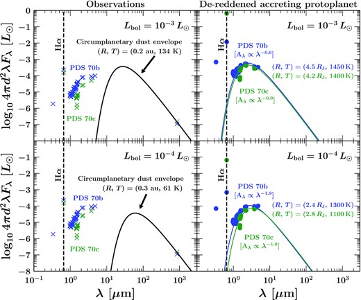
Similar to Fig. 5, but now modelling the case where the PDS 70 planets are surrounded by dusty spherical envelopes instead of circumplanetary discs. Crosses in the left-hand panels mark the observed SEDs, identical to those in Fig. 5. In the right-hand panels we show these data de-reddened, adopting a power-law extinction curve chosen so that the extinction-corrected luminosity in the U-band + H α is comparable to that in the near-infrared, with both summing to a given bolometric luminosity Lbol (|$10^{-4} \, \mathrm{L}_\odot$| for the bottom panels, |$10^{-3}\, \mathrm{L}_\odot$| for the top). These choices are intended to describe protoplanets which derive a large fraction of their luminosity from ongoing accretion, producing short-wavelength ultraviolet/optical radiation in an accretion shock that heats the planetary layers below and the circumplanetary envelope above. The blackbody fits to the de-reddened near-infrared SEDs (right panels) suggest the accretion shock lies just above ∼2–5 RJ. The circumplanetary envelope intercepts nearly all of the outgoing radiation and re-radiates it longward of 10–30 μm wavelength on size scales comparable to the Hill sphere, as shown by the blackbodies with luminosities equal to Lbol running through the mm-wave fluxes (left-hand panels). The large de-reddened U-band and optical luminosities in this figure (10−4, |$10^{-3} \, \mathrm{L}_\odot$|) are consistent with planetary accretion at Bondi-like rates and mass doubling times tdouble comparable to the system age tage.
In this extinction-free scenario the observed fluxes from the ultraviolet to the near-infrared are not significantly extincted by dust. At the same time we know the circumplanetary environment should contain dust to explain the mm-wave continuum emission imaged by Isella et al. (2019) and Benisty et al. (2021). For this mm-bright dust to not obscure our line of sight to the planet, it should be distributed in a circumplanetary disc (CPD), viewed face on or approximately so. Fig. 5 shows blackbody emission from a single-temperature CPD, heated primarily by radiation from the star to an assumed T = 60 K, with a radius fitted to the mm-wave observations. The fitted CPD radius is 0.3 au, roughly 20 per cent of the Hill sphere radius |$R_{\rm Hill} \sim 1.5\, \, \mathrm{au} \, (M_{\rm p}/M_{\rm J})^{1/3}(r/22\, \rm au)$|.
Fig. 6 shows a high-extinction scenario. Wang et al. (2020) ruled out interstellar extinction because the host star appears unextincted, and circumstellar extinction seems negligible because the planets reside within a transitional disc cavity. Thus, we are left with circumplanetary extinction, from dust brought to the planet by the nebular accretion flow, pervading the planet’s Hill sphere. To obscure our line of sight to the accretion shock, this dust should be distributed more-or-less spherically around the planet, in a geometry similar to the thick torii found in 3D hydro-simulations by Fung, Zhu & Chiang (2019, see their fig. 2). The left panels of Fig. 6 demonstrate how Hill-sphere-sized dusty spheres/torii can reproduce the measured sub-mm fluxes.
The right-hand panels of Fig. 6 show what the extinction-corrected intrinsic SED of the accreting planet might look like. We adopt power laws for how the extinction Aλ varies with wavelength λ, with the slope and normalization chosen such that the extinction-corrected luminosity in the U-band + Hα is comparable to the extinction-corrected luminosity in the near-infrared, with both summing to an assumed bolometric luminosity Lbol (|$10^{-4} \, \mathrm{L}_\odot$| for the bottom panels, |$10^{-3} \, \mathrm{L}_\odot$| for the top; see the figure annotations and caption for details). Our V-band extinction for PDS 70b is AV ≈ 2.5 for |$L_{\rm bol} = 10^{-4} \, \mathrm{L}_\odot$|, and AV ≈ 4 for |$L_{\rm bol} = 10^{-3}\, L_{\odot }$|. The de-reddened near-infrared SEDs still conform approximately to blackbodies, about as well as they do without any extinction correction applied (cf. Wang et al. 2020). Our extinction-corrected effective temperatures are higher than non-corrected values, ∼1100–1450 K versus 1000–1200 K. Our corrected planet radii are also larger, 2.4–4.5 RJ versus 2–2.7 RJ. In this interpretation the extinction-corrected near-infrared radius corresponds to the depth at which radiation emitted by the accretion shock boundary layer thermalizes, at the base of a dusty accretion flow. The analogy would be with actively accreting Class 0 protostars (e.g. Dunham et al. 2014) or ‘first’ or ‘second’ protostellar cores (Larson 1969; Bate, Tricco & Price 2014) at the centres of infalling dusty envelopes.
4 SUMMARY AND OUTLOOK
Planets are suspected to open the gaps and cavities imaged in protoplanetary discs at millimetre and infrared wavelengths. From the literature we have compiled the modelled masses Mp and orbital radii r of the putative gap-opening planets, together with local disc properties including the dust and gas surface densities Σdust and Σgas, and the gas disc thickness h. Our sample contains 22 hypothesized planets and 2 confirmed orbital companions (PDS 70b and c). From these data we have evaluated:
Present-day planetary gas accretion rates |$\dot{M}_{\rm p}$| for the subset of nine planets (including PDS 70b and c) for which the ambient gas density can be usefully constrained from molecular line observations including optically thin C18O. We assumed, consistent with some theories of planet formation, that accretion from the surrounding disc on to the planet is Bondi-like. For eight of the nine planets, accretion rates are such that mass doubling times |$t_{\rm double} \equiv M_{\rm p}/\dot{M}_{\rm p}$| are comparable to stellar ages of tage ∼ 1–10 Myr – this assumes the non-PDS 70 planets have masses |$M_{\rm p} \sim 10\rm{\!-\!}30 \, M_{\oplus }$|, the PDS 70 planets have |$M_{\rm p} \sim 1\rm{\!-\!}10\, M_{\rm J}$|, and the gas-phase CO:H2 abundance ratios are close to those found in thermo-chemical models. Since circumstellar gas discs have typical lifetimes of several Myr, our finding that tdouble/tage ∼ 1 for these eight planets suggests we are observing them during their last doublings. The one planet that does not fit this pattern is the one supposedly inside HD 163296-G2 (r = 48 au), for which we find tdouble/tage ≲ 0.1 if |$M_{\rm p} \sim 1\rm{\!-\!}10\, M_{\rm J}$| as estimated by Zhang et al. (2018). We suggest the true planet mass in this gap is smaller, and could actually be zero if the gap is created by a planet located elsewhere, following Dong et al. (2018).
Gas surface densities Σgas at the bottoms of 24 gaps where planets are supposed to reside. For 9 systems we compiled literature estimates of Σgas based on observed C18O intensity maps. For the remaining 15 systems we inferred Σgas assuming the gaps host planets undergoing Bondi accretion at the average rate Mp/tage. The predicted gas surface densities range from |$10^{-4}\, \rm g\, cm^{-2}$| to |$1\, \rm g\, cm^{-2}$|.
Dust surface densities Σdust and dust-to-gas ratios Σdust/Σgas inside gaps. In many cases Σdust/Σgas based on observations are supersolar, by contrast to the typically subsolar ratios found at the bottoms of dust-filtered gaps in planet–disc simulations (Dong et al. 2017). We suggest Σdust may be overestimated by the current ALMA observations as they may not be resolving steep dust gradients inside gaps (see also Jennings et al. 2021). Under-resolution is less of a problem for Σgas in so far as simulations predict gas gradients to be shallower than dust gradients.
Accretion luminosities Lacc of protoplanets. For the PDS 70 planets we predict |$L_{\rm acc} \sim 10^{-4}\, L_{\odot }$|, a factor of 10-100 larger than observed in the U-band and Hα. Most of the short-wavelength accretion power might be emitted in wavebands as yet unobserved, e.g. H Ly α as predicted by recent accretion shock models (Aoyama et al. 2021). Alternatively, a dusty, quasi-spherical, circumplanetary envelope might be absorbing much of the outgoing ultraviolet/optical radiation. We sketched different spectral energy distributions (SEDs) based on these scenarios. A large fraction of the power is expected to emerge at wavelengths ranging from the mid- to far-infrared.
The hypothesis that the disc substructures imaged by ALMA are caused by embedded planets is now supported on several grounds. A planet can reproduce the observed positions of multiple gaps in a given system (e.g. in AS 209; Dong et al. 2017, 2018; Zhang et al. 2018). A planet can also reproduce observed non-Keplerian velocity signatures in the disc rotation curve (e.g. in HD 163296; Teague et al. 2018, 2021; Pinte et al. 2020). To this evidence favouring planets we can now add consistency with planet accretion theory. The data are pointing to Neptune-mass planets accreting at Bondi-like rates inside gaps filled with low-viscosity (α ≲ 10−4) gas.
From here there are any number of avenues for future investigation. To list just a few:
Advancing beyond our Bondi-inspired formula (3) for |$\dot{M}_{\rm p}$|. Bondi accretion neglects many effects, among them stellar tides that become important when the planet’s Bondi radius exceeds its Hill radius (e.g. Rosenthal et al. 2020), anisotropic 3D flow fields (e.g. Cimerman, Kuiper & Ormel 2017), and thermodynamics (e.g. Ginzburg & Chiang 2019a who distinguished between hydrodynamic and thermodynamic runaway). The sensitivity of simulated accretion rates to sink-cell (e.g. D’Angelo et al. 2003) and other planetary boundary conditions should be studied.
Accounting for how the gap density evolves with time because of disc photoevaporation, repulsive planetary torques, etc., while the planet accretes. For example, in the gap clearing theories of Ginzburg & Chiang (2019a), the planet mass doubling time-scale tdouble is longer than the instantaneously measured |$M_{\rm p}/\dot{M}_{\rm p}$| by a factor that ranges up to ∼15, increasing as the disc viscosity decreases and the gap depletes more rapidly with time. This correction factor based on disc evolution should be incorporated into comparisons between tdouble and tage.
More molecular line data to test our predictions for Σgas, and higher spatial resolution to map steep Σdust profiles. New data are now available for the GM Aur disc, including spatially resolved dust continuum and CO observations (Huang et al. 2020, 2021; Schwarz et al. 2021), anchored by a total disc gas mass estimate from HD emission (McClure et al. 2016). Spatially resolved disc surveys have so far targeted brighter discs (Andrews et al. 2018; Oberg et al. 2021) and are consequently biased toward higher Σgas. Assuming planets will always be found with tdouble/tage ≳ 1, higher Σgas corresponds to lower planet masses Mp (equation 5). By this logic, targeting less luminous, less massive discs while keeping all other factors fixed may uncover higher mass planets. In any case expanding survey samples are necessary for understanding planet occurrence rates and demographic trends (Cieza et al. 2019).
Planetary accretion shock models (Aoyama et al. 2020, 2021) need to be tested observationally across the ultraviolet-optical spectrum, with current arguments based on a single emission line (H α) replaced by joint constraints from multiple lines and the continuum. The accretion shock theory also needs to connect more smoothly to models of the cooler, infrared-emitting layers of the planet (e.g. BT-Settl; Baraffe et al. 2015); at the moment how radiation from shocked layers heats cooler layers is not accounted for (but see section A1 of Aoyama et al. 2020 for a first step). Detection of molecular absorption lines in the infrared (Cugno et al. 2021; Wang et al. 2021) may constrain the degree of accretional heating, and how much dust is brought in.
ACKNOWLEDGEMENTS
We thank Yuhiko Aoyama, Steve Beckwith, Jenny Calahan, Yayaati Chachan, Ruobing (Robin) Dong, Jeffrey Fung, Sivan Ginzburg, Jane Huang, Masahiro Ikoma, Gabriel-Dominique Marleau, Jason Wang, Ke (Coco) Zhang, Shangjia Zhang, Yifan Zhou, and Zhaohuan Zhu, for discussions and feedback on our study. We also thank Takayuki Muto for a helpful referee report. This work was supported by an NSF Graduate Research Fellowship (DGE 2146752) and used the matplotlib (Hunter 2007) and scipy (Virtanen et al. 2020) packages.
DATA AVAILABILITY
The data compiled in this work are available upon request to the authors.
Footnotes
The ALMA continuum data used in our study were taken at wavelengths ranging from 0.85 mm to 1.27 mm. Our adopted factor-of-seven uncertainty in κ is larger than the expected variation of κ across this wavelength range (at fixed grain size), so for simplicity we ignore the wavelength dependence on κ when computing Σdust from the ALMA observations.
The values of h obtained by Zhang et al. (2021), if interpreted as a standard isothermal hydrostatic disc gas scale height, imply gas temperatures that differ from the gas temperatures obtained from thermo-chemical and radiative transfer modelling by these same authors (their fig. 7). This is because the latter temperatures are solved assuming a fixed density field (specified by h), and no provision is made to iterate the density field to ensure simultaneous hydrostatic and radiative equilibrium. There is no rigorous justification for using either set of temperatures to compute the gas scale height; we use h as tabulated by Zhang et al. (2021) for convenience (their parameters H100 and ψ in table 2, inserted into their equation 3 with χ = 1).
In later sections, and in particular the discussion surrounding Figs 5 and 6, we will consider the possibility that the observed near-infrared emission does not arise from a planet passively cooling into empty space (as assumed by the cooling models) but one which sits below a hot accretion shock boundary layer. In this scenario our adoption of planetary masses for PDS 70b and c drawn from the passive cooling models will lead to an inconsistency. Our hope is that our estimated mass range of |$1\rm{\!-\!}10 \, M_{\rm J}$| is not seriously impacted; it should not be as long as the posited accretion luminosities are not much larger than the observed near-infrared luminosities (|$10^{-4} \, \mathrm{L}_\odot$|; Wang et al. 2020). It may also help to have the accretion columns be localized to ‘hot spots’ on the planet, like they are for magnetized T Tauri stars (e.g. Gregory et al. 2006), leaving the rest of the planet passively cooling.
Wang et al. (2020) derived these radii by fitting blackbodies to the near-infrared spectral energy distributions of PDS 70b and c assuming no extinction. The radii may change by order-unity factors if there is circumplanetary extinction, as proposed later in this section.
