


ABSTRACT
When a star passes close to a supermassive black hole (BH), the BH’s tidal forces rip it apart into a thin stream, leading to a tidal disruption event (TDE). In this work, we study the post-disruption phase of TDEs in general relativistic hydrodynamics (GRHD) using our GPU-accelerated code h-amr. We carry out the first grid-based simulation of a deep-penetration TDE (β = 7) with realistic system parameters: a black hole-to-star mass ratio of 106, a parabolic stellar trajectory, and a non-zero BH spin. We also carry out a simulation of a tilted TDE whose stellar orbit is inclined relative to the BH midplane. We show that for our aligned TDE, an accretion disc forms due to the dissipation of orbital energy with ∼20 per cent of the infalling material reaching the BH. The dissipation is initially dominated by violent self-intersections and later by stream–disc interactions near the pericentre. The self-intersections completely disrupt the incoming stream, resulting in five distinct self-intersection events separated by approximately 12 h and a flaring in the accretion rate. We also find that the disc is eccentric with mean eccentricity e ≈ 0.88. For our tilted TDE, we find only partial self-intersections due to nodal precession near pericentre. Although these partial intersections eject gas out of the orbital plane, an accretion disc still forms with a similar accreted fraction of the material to the aligned case. These results have important implications for disc formation in realistic tidal disruptions. For instance, the periodicity in accretion rate induced by the complete stream disruption may explain the flaring events from Swift J1644+57.
1 INTRODUCTION
In recent decades, several very bright flares in galactic nuclei have been observed and interpreted as tidal disruption events (TDEs), which occur when a star is scattered on to a nearly parabolic orbit around a supermassive black hole (BH) with a pericentre inside the tidal radius of the BH (Hills 1975; Frank & Rees 1976; Rees 1988). While these flares are typically discovered from quasi-thermal emission in the soft X-ray (Bade, Komossa & Dahlem 1996; Komossa & Bade 1999; Saxton et al. 2012), UV (Gezari et al. 2006, 2008), or optical (van Velzen et al. 2011; Gezari et al. 2012; Arcavi et al. 2014; Holoien et al. 2014) bands, they have been observed to emit radiation across the electromagnetic spectrum, from radio synchrotron (Zauderer et al. 2011; Alexander et al. 2017) to non-thermal hard X-rays and soft gamma rays (Bloom et al. 2011; Cenko et al. 2012; Brown et al. 2015).
Our current theoretical understanding of the tidal disruption process – the star’s first, terminal pericentre passage – is largely converged (Lacy, Townes & Hollenbach 1982; Carter & Luminet 1983; Guillochon & Ramirez-Ruiz 2013; Mainetti et al. 2017), at least for polytropic stars in Newtonian gravity. More recent simulations have explored how the immediate outcome of disruption depends on stellar spin (Golightly, Coughlin & Nixon 2019a; Kagaya, Yoshida & Tanikawa 2019), realistic models of the star’s internal structure (Golightly, Nixon & Coughlin 2019b; Ryu et al. 2020a), and general relativistic gravity (Gafton et al. 2015; Tejeda et al. 2017; Gafton & Rosswog 2019; Ryu et al. 2020b). However, we do not yet have a first principles understanding of how, or if, the stellar debris streams are able to form a nearly axisymmetric, or quasi-circular, accretion disc (for a recent review of this problem see Bonnerot & Stone 2020). Because the bound stellar debris has typical eccentricities 0.99 ≲ e ≲ 0.999 (Stone, Sari & Loeb 2013), an enormous excess of orbital energy must be dissipated for circularization to occur.
Early work conjectured that most of this energy dissipation arises from relativistic apsidal precession (Rees 1988): as the most tightly bound debris passes through pericentre, its apsidal angle measured in radians precesses by an order-unity amount, causing a large-angle collision with less tightly bound matter that has yet to return to pericentre. The shocks that thermalize bulk kinetic energy at the point of self-intersection offer a plausible mechanism for circularizing returning stellar debris (Hayasaki, Stone & Loeb 2013; Bonnerot et al. 2016). However, self-intersection shocks may be less efficient at circularizing the debris for inclined orbits around spinning Kerr BHs. In this regime, nodal precession, due to Lense–Thirring frame dragging may delay the onset of self-intersection by many orbits (Cannizzo, Lee & Goodman 1990; Kochanek 1994; Guillochon & Ramirez-Ruiz 2015; Hayasaki, Stone & Loeb 2016). Additionally, energy dissipation due to self-intersection shocks may be greatly limited for less relativistic orbital pericentres, with small-angle collisions occurring at self-intersection radii near the apocentre of the most tightly bound debris (Dai, McKinney & Miller 2015; Shiokawa et al. 2015).
An alternative dissipation site is at the stream pericentre itself, where the recompression of the returning debris generates ‘pancake’ or ‘nozzle’ shocks (Kochanek 1994). Recently, Bonnerot & Lu (2021) performed an in-depth study of the nozzle shock using a 2D simulation of a vertical slice of the stream and found that dissipation at the nozzle shock raises the entropy of the gas by two orders of magnitude. Newtonian hydrodynamic simulations by Ramirez-Ruiz & Rosswog (2009) have shown that this pericentre shock could feasibly circularize the tidal debris. However, these simulations were performed for a BH-to-star mass ratio of Q = 103 and analytic estimates of Guillochon, Manukian & Ramirez-Ruiz (2014) suggest that pericentre recompression shocks become less efficient at more realistic mass ratios (e.g. Q = 106). It is also possible that in many TDEs, efficient dissipation is lacking altogether, and the formation of an accretion disc is an inefficient process unfolding over many fallback times (Piran, Sa̧dowski & Tchekhovskoy 2015). We discuss further in Section 4.1.
TDE debris circularization and disc formation is a complex physical problem involving a large dynamic range, general relativistic orbital dynamics, the need for accurate treatment of hydrodynamic shocks, and possibly even magnetohydrodynamic (MHD) effects (Svirski, Piran & Krolik 2017). The many pieces of multiscale and non-linear physics involved in TDE disc formation mean that, for numerical reasons, almost all past simulations of this process employed major simplifying assumptions that cast doubt on the generality of their conclusions.
Ayal, Livio & Piran (2000) initiated the numerical study of TDE circularization using a post-Newtonian (PN) potential to simulate the lowest order level of apsidal precession in a finite-mass, smoothed particle hydrodynamics (SPH) framework, albeit with low (N ∼ 103) particle number. More recently, global circularization simulations achieved much higher resolution by reducing the dynamic range of the problem in one of two ways. The first is to consider an unrealistically low mass ratio, typically Q ∼ 103. In simulations of this type, general relativity is sometimes ignored completely (Guillochon et al. 2014), but when it is included, it has a minimal effect on the circularization process because the tidal radius around an intermediate-mass BH is not very relativistic (Ramirez-Ruiz & Rosswog 2009; Shiokawa et al. 2015).
The second option is to consider a realistic mass ratio (Q ∼ 106) but an unrealistic pre-disruption stellar orbit. Tidally disrupted stars typically approach supermassive BHs on nearly parabolic orbits (Magorrian & Tremaine 1999), with initial eccentricities 1 − e0 ∼ 10−5. For computational convenience, one may choose an unrealistic stellar eccentricity, e0 ≲ 0.95, to reduce the debris stream apocentres. This approach was adopted by Hayasaki et al. (2013), who mimicked apsidal precession effects with a pseudo-Newtonian potential in a highly relativistic β = 5 TDE. They found rapid circularization due to orbital energy dissipation at stream self-intersections. Later simulations found that in less relativistic β = 1 TDEs, self-intersections are less efficient at energy dissipation compared to this initial work (Bonnerot et al. 2016).
The results of Hayasaki et al. (2013) were later confirmed and extended to different gas equations of state (Bonnerot et al. 2016; Hayasaki et al. 2016), as well as higher (but still sub-parabolic) eccentricities (Bonnerot et al. 2016; Sądowski et al. 2016). The low-e0 limit of tidal disruption has also been used with PN potentials to include Lense–Thirring frame dragging, which was seen to substantially delay circularization provided debris streams remain thin (Hayasaki et al. 2016). More recently, Bonnerot & Lu (2020) have performed a TDE disc formation simulation with realistic astrophysical parameters using a different approximation: neglecting the returning debris streams entirely, and injecting mass, momentum, and energy (in the form of SPH particles) from the test-particle self-intersection point. The validity of this approach depends on the accuracy of the local injection scheme, and its independence from global gas evolution around the BH. We discuss this approach further and compare and contrast it to our results in Section 4.5.2.
In this paper, we use novel numerical techniques to capture the disc formation process in general relativistic hydrodynamics without sacrificing astrophysical realism in our choice of system parameters (e.g. Q, e0). We use two-level adaptive mesh refinement (AMR) to resolve the relevant physics within our grid-based code. In Section 2, we outline our numerical scheme. In Section 3, we describe the general outcomes of our simulation, including the spatial properties of the nascent accretion flow. In Section 4, we more carefully analyse the specific physical mechanisms controlling the accretion and circularization process and provide a detailed comparison to the ZEro-BeRnoulli Accretion (ZEBRA) model of Coughlin & Begelman (2014). We conclude in Section 5.
2 NUMERICAL METHOD AND SETUP
We simulate the initial tidal disruption using the SPH code phantom (Price & Monaghan 2007) and we simulate the post-disruption evolution using our new GRMHD code h-amr (Liska et al. 2019), an approach analogous to those of Rosswog, Ramirez-Ruiz & Hix (2009) and Sądowski et al. (2016). With this hybrid method, we can account for the large range of spatial and temporal scales involved in the disruption process and debris stream formation while accurately capturing the essential shocks and general relativistic effects in the post-disruption evolution.
2.1 Initial disruption in phantom
The stellar disruption is initially followed by the smoothed-particle hydrodynamics code phantom (Price et al. 2018). The setup is identical to that described in Coughlin & Nixon (2015): a star of mass |$1\, {\rm M}_{\odot }$| is modelled as a γ = 5/3 polytrope, with the adiabatic index equal to the polytropic index, by placing ∼107 particles on a close-packed sphere. The sphere is stretched to achieve roughly the correct polytropic density profile. The star is subsequently relaxed in isolation (i.e. without the external gravitational potential of the BH) for ten sound crossing times to smooth out numerical perturbations in the density profile. Self-gravity is included through the implementation of a tree algorithm alongside an opening angle criterion to calculate short-range forces (Gafton & Rosswog 2011). We also include the effects of shock heating in modifying the internal energy of the gas.
The initial, parabolic orbit of the star is established using the above potential (equation 1) to calculate the angular momentum necessary to achieve a pericentre distance of rp = 7Rg. phantom uses an artificial viscosity prescription to mediate any strong shocks that may be present during the large compression suffered by the star and employs the standard switch proposed by Cullen & Dehnen (2010) (i.e. the artificial viscosity parameter is small when the star is far from pericentre and approaches values near unity as the star is compressed at pericentre). A non-linear term is also included to account for extremely strong shocks and prevent interparticle penetration (Price & Federrath 2010). The large number of particles (∼107) was used to avoid the possibility of spurious numerical heating at pericentre caused by under-resolving the compression, predicted to be of the order of Hmin/R* ∼ β−3 ∼ 0.003 (Carter & Luminet 1983), though the compression could be smaller if shock heating halts the otherwise-adiabatic collapse (Bicknell & Gingold 1983), or due to 3D effects (Guillochon et al. 2009). Here β = rt/rp is the penetration factor, rt is the tidal radius, and rp is the pericentre radius.
Fig. 1 shows the density distribution of the disrupted stellar debris at 1.16 d after the disruption. At this time, we end the evolution of the TDE in phantom and use the distribution of debris as the initial conditions for our post-disruption simulation in h-amr. See Section 2.2 for a detailed description of how we map data from SPH to grid-based GRHD.
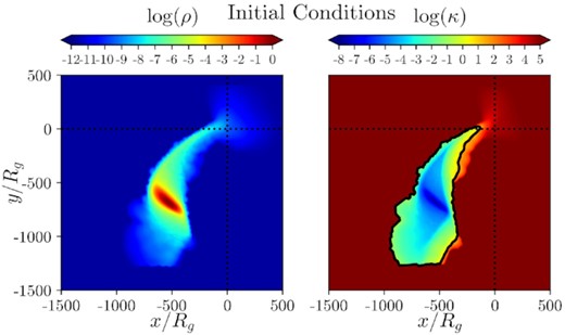
Colour maps of the log of rest mass density and log κ (proportional to entropy, see equation 7), in the equatorial plane at the initial conditions of the post-disruption phase of the simulation in h-amr (1.16 d). The black contour on the right-hand panel outlines the area excluded by the entropy condition (κ < 10) which we use throughout our analysis to distinguish the material in the debris stream from the material in the accretion disc). The BH is located at the origin. The dotted lines indicate the x- and y-axes.
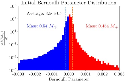
A histogram of the Bernoulli parameter distribution at the initial conditions of the post-disruption phase of the simulation in h-amr (1.16 d). Each bin is weighted by solar masses and bin width. Unbound material and total unbound mass are shown in red; bound material and total bound mass are shown in blue. The mass-weighted average Bernoulli parameter is also shown. On average, the material in the initial conditions of the post-disruption phase is marginally bound (b = 0). The vertical lines represent the range of the Bernoulli parameter estimated from the frozen-in approximation (equation 3), and contain 98.1 per cent of the debris mass. The floor material is ignored using a density condition (ρ > 10−11).
A small fraction of the material has Bernoulli parameters well outside the range predicted by the frozen-in approximation. However, even though the most tightly bound debris (with specific energy |ε| > Δb) constitutes a small fraction of the total mass, it is the first matter to fall back, and therefore dominates the early stages of the circularization process studied here. Due to runtime limitations, these early stages are the primary focus of this paper. While these tails could be a byproduct of intense shock heating as the star is highly compressed near pericentre, we caution that they may also arise from numerical inaccuracies associated with the same highly compressed, and therefore difficult to resolve, configuration of gas.
Such broad-energy tails have been seen in high-β TDEs simulated with a range of codes and numerical algorithms. While a return time of 1.16 d for the most tightly bound debris might appear extreme, it is qualitatively consistent with these past simulations. For example, Guillochon & Ramirez-Ruiz (2013) find that the most tightly bound debris in Newtonian, grid-based, β = 4 simulations of n = 3 polytrope disruptions can return to pericentre after ≈3 d and that the time of first pericentre return decreases with increasing β. Steinberg et al. (2019) performed moving-mesh simulations of stellar disruptions and found that the extent of the high energy tail is also a function of β. For Newtonian disruptions of n = 3/2 polytropes, going from β = 5 to β = 7 moves the time of first mass return from ≈3 d to ≈1 d (Steinberg, private communication). Gafton & Rosswog (2019) used Newtonian and relativistic SPH simulations, with a code distinct from phantom, to disrupt a γ = 5/3 polytrope over a range of β and found that for large β the return time of the most bound debris was significantly earlier than the frozen-in prediction, with initial return times on the order of days.
These high-energy, low-mass debris tails have not been studied in detail, but their ubiquity across SPH, conventional grid-based, and moving mesh codes leads us to believe that they are likely physical. If, however, the high-energy tail of debris were primarily the result of numerical artefacts, then it would bias the earliest stages of mass return to (i) artificially early times and (ii) artificially low fallback rates relative to the time of first mass return.
However, our results depend solely on the relative values of mass fluxes rather than the absolute values, with the exception of the internal energy and density floors (Section 2.3). Therefore, even if the mass of the high-energy tail of debris in our initial conditions is an overestimate, our results can be straightforwardly rescaled to astrophysically realistic time and mass flux scales (i.e. our simulation would have started at a later time with similar values of relative mass flux). The qualitative features of the circularization process are therefore robust and should apply generically to systems with realistic physical parameters and β ≃ 7.
2.2 Mapping from phantom to h-amr
Before we begin our simulations in h-amr, we map SPH data from phantom to gridded data compatible with GRHD. First, smooth the particle properties on to a continuous domain. Secondly, we construct a grid on top of the smoothed particles.
For the first step, we use the SPH visualization tool splash and its built-in function ‘splash to grid,’ which is described in detail in Price (2007). The function smooths the density of each particle over a finite region according to a weighting function, or kernel, that is twice differentiable, maintains compact support, and decreases in magnitude from the location of the particle. This approach mirrors the standard procedure for SPH calculations. We use the default kernel in splash (and phantom): a cubic spline which vanishes at a distance of 2h from a given particle. The smoothing length h is spatially variables and set such that the mass inside the smoothing sphere is constant. We refer the reader to section 2.4 of Price (2012) for more details.
For the second step, the fluid variables of a given cell are determined by adding the contribution of every particle with a smoothing region that encompasses the cell itself. See fig. 7 of Price (2007) for an illustration. This method ensures that cells in high-density regions are sampled by a large number of particles and cells in low-density regions are sampled by relatively few particles. Because of their low density, sparsely sampled cells contribute minimally to the dynamics of the fluid and do not affect the bulk properties of the accretion flow simulated with h-amr.
The error in the first step is of the order of |$\mathcal {O}(h^2) = \mathcal {O}(\rho ^{-2/3})$|. Therefore, in regions of extremely low density, the interpolation from SPH may introduce artefacts in the density and velocity fields. In particular, we find a region of enhanced density in the region around the black hole (Fig. 1). The density of this region is several orders of magnitude lower than the density of the most bound debris, so the trajectory of the returning debris is not significantly altered.
2.3 h-amr simulation parameters
As described in Section 1, our simulation parameters adhere to astrophysically realistic values (Q = 106, e0 ≈ 1). In phantom we insert a star on a parabolic trajectory with a pericentre distance of 7Rg and a penetration factor of β = rt/rp = 7. This high penetration encounter guarantees that self-gravity is negligible in the post-disruption evolution of the stream, although the influence of self-gravity on the stream structure may be revived at much later times than those simulated here due to the in-plane focusing of the debris; Coughlin et al. 2016; Steinberg et al. 2019). The circularization of the stellar debris likely occurs on a shorter time-scale for more relativistic encounters (Bonnerot & Stone 2020), decreasing the simulation duration required to study the circularization process.
h-amr uses a naturalized unit system where G = c = Rg = 1. The conversion factors from the simulation units to cgs units are given in Table 1. From now on, we will work in this naturalized unit system with the exception of time, which we will convert back to physical units of days since disruption. We will also restore G and c in equations to help keep track of units.
Although h-amr does not explicitly include viscosity, it is included implicitly through interactions at the cell level. Within the turbulent flows of our simulation, adjacent fluid elements are unlikely to move exactly parallel to one another and therefore will exchange momenta. Previous work has shown that the effective viscosity in early-time TDE accretion flows can be dominated by the Reynolds stress (Sądowski et al. 2016). If this is correct, we should not be significantly underestimating effective viscosity due to the absence of magnetic fields, though this question needs closer examination in future magnetohydrodynamic simulations.
For each quantity, the number of cgs units per simulation unit is tabulated. Note that 0 Rg/c corresponds to 1.16 d after the disruption, so the relationship between simulation time and days since disruption is affine linear.
| Quantity | cgs unit | h-amr unit | cgs unit / h-amr unit |
|---|---|---|---|
| Mass | g | Rgc2/G | 2 × 1039 |
| Distance | cm | Rg | 1.477 × 10¹¹ |
| Time | s | Rg/c | 4.926 |
| Density | g cm−3 | |$c^2/R_{\rm g}^2 G$| | 6.207 × 10⁵ |
| Quantity | cgs unit | h-amr unit | cgs unit / h-amr unit |
|---|---|---|---|
| Mass | g | Rgc2/G | 2 × 1039 |
| Distance | cm | Rg | 1.477 × 10¹¹ |
| Time | s | Rg/c | 4.926 |
| Density | g cm−3 | |$c^2/R_{\rm g}^2 G$| | 6.207 × 10⁵ |
Simulation parameters for models TDET0 and TDET30, including black hole mass MBH, stellar mass M*, pericentre radius Rp, penetration factor β, and inclination angle of the stellar orbit i.
| Model | MBH (M⊙) | M* (M⊙) | Rp (Rg) | β | i |
|---|---|---|---|---|---|
| TDET0 | 106 | 1 | 7 | 7 | 0 |
| TDET30 | 106 | 1 | 7 | 7 | 30 |
| Model | MBH (M⊙) | M* (M⊙) | Rp (Rg) | β | i |
|---|---|---|---|---|---|
| TDET0 | 106 | 1 | 7 | 7 | 0 |
| TDET30 | 106 | 1 | 7 | 7 | 30 |
In both models, we use a dimensionless BH spin of a = 0.9375 for the post-disruption evolution. Because the morphology and the fallback rate of our stream are not strongly dependent on spin (Tejeda et al. 2017), we rotate the initial data in h-amr about the y-axis by 30 deg for model TDET30 rather than repeating the simulation in phantom. We take this approach, rather than tilting the metric, to avoid the computational strain associated with a non-axisymmetric metric.
We run models TDET0 and TDET30 until 6.87 d (t = 105Rg/c in h-amr) and 5.01 d (t = 6.7 × 10⁴Rg/c in h-amr) after the disruption, respectively. We evolve the models in the Kerr geometry using Kerr-Schild coordinates to avoid the coordinate singularity in the Boyer-Lindquist coordinates.
In addition to AMR, h-amr uses local adaptive time stepping by setting the time-step in each cell to the smallest light crossing time in that cell. As a result, the time-steps decrease by a factor of Δϕ/Δθ near the pole due to the time-step limitation in φ. Therefore, we use the cylindrification method described by Tchekhovskoy, Narayan & McKinney (2011) to reduce the azimuthal extent of cells near the pole.
As we ran the simulation, we noticed that the stream disintegrates into the accretion disc after wrapping around the BH, a behaviour which we discuss more in Section 3.1. To verify that this stream disintegration was not a numerical artefact, we adjusted the refinement criterion for first-order refinement between 2.28 d (4 × 10⁴Rg/c) and 4.56 d (8 × 10⁴Rg/c). Near the BH, we decreased the cutoff density for first-order refinement to achieve the full effective resolution in a greater fraction of cells. Due to memory restrictions, we also had to increase the cutoff density at large radii, causing some parts of the outer stream to become unrefined. We found that the stream disintegration and other simulation properties were consistent across adjustments to the refinement criterion, suggesting that the physics converged for our resolution in h-amr.
In the post-disruption phase, we set floors for internal energy density and mass density at 2.27 × 10⁻¹² (3.75 × 10⁶ ergs cm−3 and 4.167 × 10⁻¹⁵ g cm−3 respectively). We assume an adiabatic index γ = 5/3 corresponding to the gas-pressure-dominated regime present in the star before it undergoes shocks. Although any accretion disc resulting from the TDE is expected to be radiation-pressure-dominated with an adiabatic index closer to γ = 4/3, h-amr currently does not allow for a variable adiabatic index so we chose to stay consistent with the initial simulation in phantom. Many previous works have also used an adiabatic index of γ = 5/3 (Guillochon & Ramirez-Ruiz 2015; Sądowski et al. 2016; Steinberg et al. 2019). In future simulations, we will implement a variable adiabatic index to more accurately model the thermodynamics.
3 RESULTS
3.1 Aligned disc formation and evolution
General relativistic apsidal precession near the BH causes the argument of pericentre to advance by approximately 31°, setting the incoming and outgoing streams on trajectories that intersect at RSI = 142Rg. The precession angle and self-intersection radius are computed with the formalism in Appendix A4.
Shortly after the first pericentre passage, depicted in the first row of Fig. 3, the debris stream expands significantly and its density drops. The primary reason for this expansion is the different degrees of apsidal precession experienced by the inner- and outer-most edges of the stream. For instance, at t = 1.25 d (top right-hand panel of Fig. 3), the inner and outer edges of the stream at pericentre lie at r = 11Rg and r = 21Rg respectively, resulting in a difference of roughly 15° in their precession angle (Fig. 4). Bonnerot & Lu (2021) discuss this effect as being potentially responsible for a small amount of spreading of the debris following its first return to the initial point of disruption. Here, because the pericentre distance of the star is much more relativistic than the modest-β case that they considered, the differential precession is larger than they find and apparent by eye.
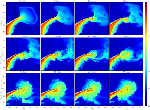
Contour plots of the log of rest mass density in the equatorial plane in the TDET0 simulation during the debris’ initial pericentre passage (first row) and the first (second row) and third (third row) self-intersection events. In the initial pericentre passage, the stream falls back through near vacuum and matter from the stream begins to accumulate near the BH. In the self-intersection events, the stream undergoes apsidal precession and self-intersects close to the analytical self-intersection radius at 142Rg. As a result, the inner parts of the stream are completely disrupted. These violent events are a key dissipation mechanism in the early stages of the TDE evolution. Although powerful, we count only five such events. At late times in our simulation, dissipation occurs primarily through interactions with the newly formed disc (Fig. 5). For a more complete picture of the disc evolution, see the movies and 3D renderings linked in Section 6.
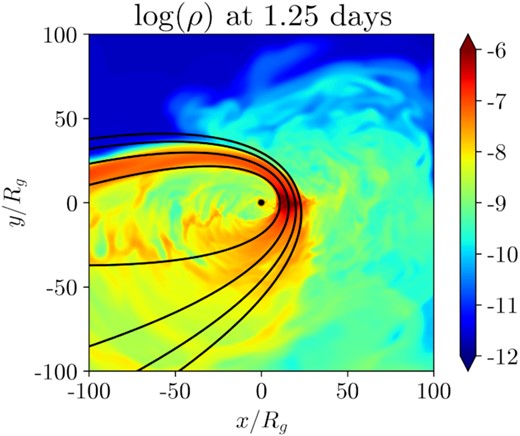
A contour plot of the log of rest mass density in the equatorial plane at 1.25 d (1725Rg/c; same as the top right-hand panel of Fig. 3) with equatorial geodesics of various pericentre radii. The geodesics diverge after pericentre, demonstrating the strong effect of differential precession in expanding the stream in the deeply penetrating (β = 7) and high-spin (a = 0.9375) encounter we consider.
Over the course of the simulation, the self-intersection periodically becomes powerful enough to fully intercept the incoming debris stream. During these violent self-intersection events, the collision of the incoming and outgoing streams and the associated shock heating nearly destroys the stream interior to the self-intersection point and ejects material into a wide range of orbits. Rows two and three of Fig. 3 depict the time evolution of two such intersection/depletion cycles.
However, once the accretion disc becomes sufficiently dense and massive, no additional violent self-intersections occur because the outgoing stream completely disintegrates before the self-intersection point as in Fig. 5. At late times, the spread in angular momenta within the incoming stream grows due to angular momentum exchange with the accretion disc. As a result, the stream becomes thicker, enhancing the effect of differential precession discussed earlier in this section. The result is that the outgoing stream has a larger spread in trajectories and a lower density than the incoming stream. At even later times, the disc is sufficiently dense to absorb nearly all of the momentum from the weakened outgoing stream through shocks and hydrodynamic instabilities at the interface. In particular, the velocity difference between the outgoing stream and the disc leads to a Kelvin–Helmholtz instability (see Bonnerot & Stone 2020, section 2.2.4), which seeds turbulence in the outgoing stream causing it to break apart.
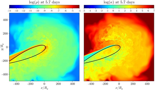
Contour plots of the log of rest mass density density (left-hand panel) and κ (right-hand panel) in the equatorial plane at 5.7 d. At late times in the simulation, the debris stream undergoes shocks and instabilities near pericentre, causing it to disintegrate shortly after the pericentre passage. This is different from the stream’s early time evolution (Fig. 3), possibly because an inner accretion disc has formed with density comparable to the incoming stream. The black line depicts an equatorial geodesic (Appendix A2). Note that the self-intersection radius of the geodesic is much greater than the analytical self-intersection radius of 142Rg for a pericentre of 7Rg because the geodesic has a larger pericentre radius of ∼12Rg.
At early times, especially before substantial disc formation, the pericentre radius undergoes fluctuations. From the movies linked in Section 6, we see that the outward movements of the pericentre coincide with the onset of a violent self-intersection. This suggests that the pericentre movement results from the azimuthal momentum added to the incoming stream by the outgoing stream during a self-intersection. After the self-intersections cease, the pericentre radius becomes more stable and takes on a value around 12Rg (corresponding to a self-intersection radius RSI = 565Rg). This may be because the outgoing stream has a weaker, but more stable, contribution to the azimuthal momentum of the incoming stream at late times.
Instead of forming a standard, geometrically thin disc, the material surrounding the black hole is inflated into a geometrically thick structure that is both gas-pressure and centrifugally supported. We perform a more in-depth analysis of the force balance in the disc and the disc structure in relation to analytical models in Sections 4.4 and 4.5.
The tidal compression of returning debris streams is approximately a reversible process, so entropy is nearly constant until the first shock. For the purposes of analysis, we define the stream as material with κ < 10, a definition we refer to as the entropy condition. Fig. 1 depicts an entropy profile of the stream at the initial conditions of the post-disruption phase in the equatorial slice. The black contour outlines the area covered by the entropy condition.
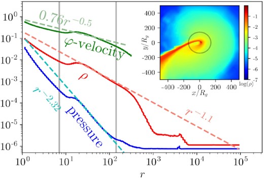
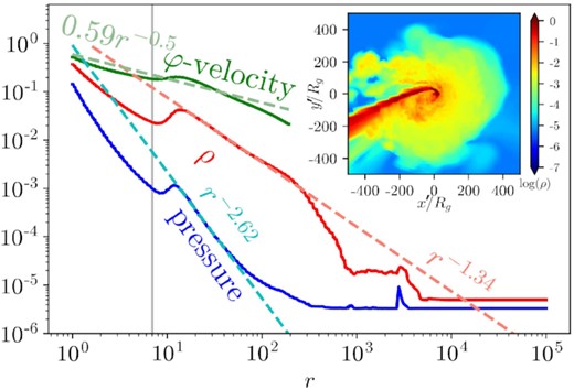
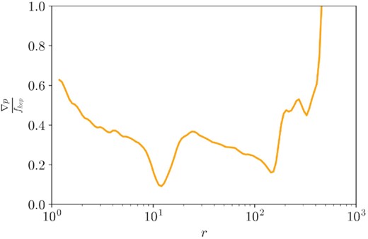
Time averages of radial profiles of mass density, pressure, and φ-velocity, their power-law fits, and an inset plot of time-averaged rest mass density in the equatorial plane. Power-law fits (dashed lines) are calculated using a least-squares method (see Table B1 for more details). Time averages are over the simulation’s full duration. Mass density, pressure, and φ-velocity are averaged over spherical shells using equation (11). Pressure and φ-velocity are weighted by mass. The stream is ignored using the entropy condition. Mass, density, and pressure are multiplied by 5 × 10⁵ so that all three variables are roughly the same order of magnitude for ease of comparison. The vertical lines show the pericentre radius at 7Rg and the analytical self-intersection radius at 142Rg (Appendix A4). The analytical self-intersection radius is also shown on the inset plot. All three quantities follow power-law fits within the radii of the disc. The sub-unity coefficient on the φ-velocity indicates that the disc is sub-Keplerian. At radii less than the pericentre radius or greater than 400 Rg, there is minimal disc material, so the data at these radii does not reflect the large-scale properties of the disc. The origin of the flat density and pressure regions at large radii (r ≳ 1000Rg) is due to the choice of the floors. The origin of the dips in all quantities at small radii is due to the absence of disc material in the plunging region.
Fig. 6 shows that the radial profiles (i.e. averaged over angles) of density and pressure closely follow power-law relationships between the inner and outer boundaries of the disc (10–200 Rg), hinting at a possible analytic description (see Section 4.5.1). The angle-averaged φ-velocity is fitted by vφ ≃ 0.76r−0.5, which implies a sub-Keplerian velocity distribution that may be due to thermal pressure support against gravity (see Section 4.4).
The internal energy density and mass density are floored at 2.27 × 10⁻¹² (see Section 2.3). These floors are responsible for the flat density and pressure regions at large radii in Fig. 6. While these floors would have a negligible effect on a TDE at peak fallback rate, they become significant for the early times and low fallback rates considered in our simulation. The floors may affect our results by providing external pressure support to the outer disc, artificially lowering its radial and vertical extent. We discuss this in Section 4.5.1.
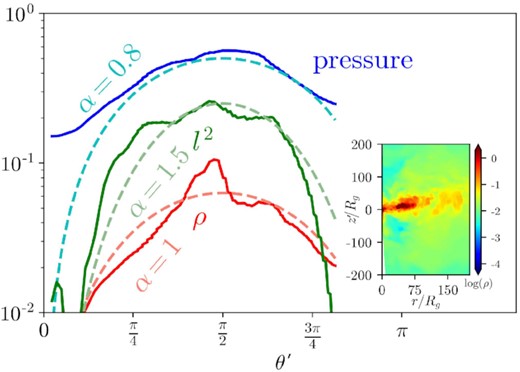
Fig. 7 shows the polar profiles of density, pressure, and squared specific angular momentum within the disc. We calculate the pressure as above (equation 9) and the specific angular momentum as l = uϕ. The polar profiles of all three quantities are fit to a power α of sin 2θ near the equatorial plane. We analyse these relationships further and compare them to model predictions in Section 4.5.1.
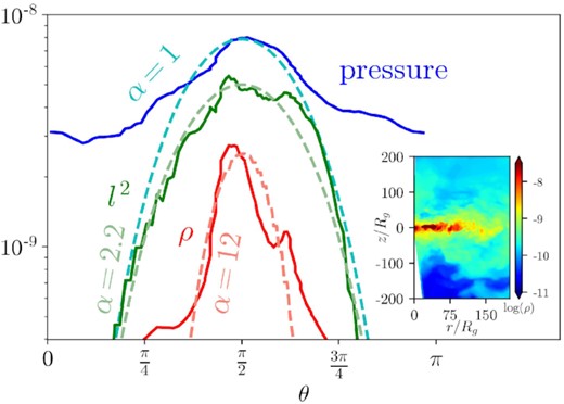
Mass density, pressure, and angular momentum squared in our aligned TDET0 model plotted with respect to θ, their fits to a power law of sin 2θ, and an inset plot of rest mass density in the xz-plane at 5.7 d. Curve fits are estimated by eye and shown in dashed lines. α represents the exponent of a power law of sin 2θ. Angular momentum is normalized in radius with a factor of r−1/2. Density, pressure, and angular momentum are averaged over φ and 10 < r < 100 using equation (11). Pressure and angular momentum are weighted by mass. The stream is ignored using the entropy condition. Density, pressure, and angular momentum squared are multiplied by 0.158, 316, and 10−8 respectively so that all three quantities are roughly the same order for comparison purposes.
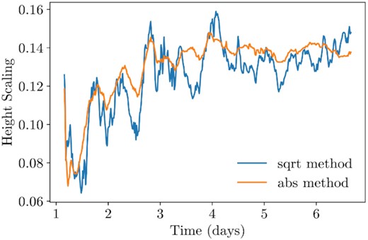
The scale height of the disc plotted with respect to time in our aligned TDET0 model. Scale height is calculated by averaging the mass-weighted angle from the equatorial plane over |θ − π/2| < 0.3 and φ using two methods described by equations (13) and (14). The stream is ignored using the entropy condition. The generation of thermal energy due to stream–disc interactions and self-intersection shocks causes the gas in the disc to expand over time, increasing the scale height.
Both methods show that h/r increases over time, indicating that the disc ‘puffs up’ from the midplane. Although it is possible that the vertical expansion of the disc is artificially slowed by the pressure and density floors, this effect should not significantly impact this general trend. The increase in the angular extent of the material is due to excess thermal energy generated in the disc by the dissipation of orbital energy. The scale height reaches a plateau around the time that the self-intersections stop (3.68 d), suggesting that the violent self-intersections play a crucial role in the early heating of the disc. We discuss the mechanisms of energy dissipation further in Section 4.1.
3.2 Tilted disc formation and evolution
The majority of TDE disc formation simulations use either Newtonian gravity or a general relativistic treatment (exact or approximate) of a non-spinning Schwarzschild BH. However, tidally disrupted stars approach the BH from a quasi-isotropic distribution of inclinations, highlighting the importance of more general disc formation simulations that account not just for BH spin, but also for spin-orbit misalignment. Various effects unique to tilted accretion discs, such as global precession, Bardeen–Petterson alignment, and disc tearing (Nixon & King 2012; Hawley & Krolkik 2019; Liska et al. 2021) may all manifest themselves in TDE accretion discs. Although previous studies have considered tilted TDEs analytically (Stone & Loeb 2012; Zanazzi & Lai 2019), only two numerical efforts have, to date, simulated the formation of an accretion flow following the disruption of a star on a misaligned orbit: the early work of Hayasaki et al. (2016), and the more recent simulations of Liptai et al. (2019). In both cases, the authors find that for adiabatic gas equations of state, it is challenging for nodal precession to cause significant delays in self-intersection. However, both of these simulations employed unrealistically eccentric stellar trajectories for computational convenience; the work presented in this section is the first numerical simulation of tilted TDEs with realistic astrophysical parameters.
The movie and 3D rendering (Section 6) of the tilted TDE shows that, unlike in the aligned TDE, the returning stream is never completely interrupted by self-intersections. The misalignment between the orbital plane of the stream and the rotational plane of the BH leads to strong nodal precession upon pericentre passage. The outgoing stream exits the BH in a separate plane from the incoming stream, so when the two streams collide, they are misaligned. Fig. 9 shows that this misalignment launches material from both streams out of their original planes.
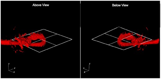
A 3D contour of density (ρ = 10−8) visualized at 3.7 d in our tilted TDET30 model. We show the views from above and below the BH orbital plane in the left-hand and right-hand panels, respectively. The outgoing and incoming streams are misaligned at the self-intersection point due to the nodal precession at the pericentre passage. As a result, material is ejected out of the orbital plane of the star. The orbital plane of the BH is shown for reference. To see this effect in the full context of disc formation, see the 3D renderings linked in 6.
Fig. 10 shows that the radial profiles of the tilted disc follow similar power-law relationships to those of the aligned disc, with the density and pressure falling off slightly faster in the aligned disc. As a result, the thermal pressure gradient forces in the tilted disc are larger than in the aligned disc, so the velocity distribution is more sub-Keplerian.
From a comparison of the polar density profiles of the aligned and tilted TDE (Figs 7 and 11), the accretion disc appears significantly thicker in the tilted simulation. However, there are two caveats to this interpretation of the data. First, the launching of stream material into different orbital planes as shown in Fig. 9 creates pockets of high density material at large polar angles which artificially increases our estimates of disc thickness. Secondly, the disc material may lie in multiple orbital planes because debris which falls back at early times has more time to undergo nodal precession than debris which falls back at late times. Any dependence of the inclination angle on r or ϕ would artificially increase our estimate of disc thickness. Additionally, the angular momenta of the gas may not have enough time to homogenize because the simulation was not run for multiple viscous times of the disc.
Analogous to Fig. 6, but for the tilted TDE simulation, model TDET30. The data are tilted using our tilting algorithm (Appendix C) such that the star’s orbital plane coincides with θ′ = π/2. Coordinates in the tilted frame are denoted with a prime. The inset plot shows the rest mass density in the star’s orbital plane at 4.0 d. See Table B2 for more details about the power-law fits (dashed lines). Mass density and pressure are multiplied by 5 × 10⁵ so that all three variables are roughly the same order for comparison purposes.
Analogous to Fig. 7, but for the tilted TDE simulation, model TDET30. The data are tilted using our tilting algorithm (Appendix C) such that the star’s orbital plane coincides with θ′ = π/2. Coordinates in the tilted frame are denoted with a prime. Density and pressure are multiplied by 107.3 and 1010.7 respectively so that all three quantities are roughly the same order for comparison purposes. The tilt angle varies over radius and time (Fig. 23), so the averages may not accurately reflect the thickness of the disc.
4 DISCUSSION
4.1 Energy dissipation
The largest uncertainty in TDE evolution concerns the rate, location, and physical mechanisms that dissipate the orbital energy of dynamically cold debris streams. Past analytic models and numerical simulations examining early stages of a TDE generally focus on shock dissipation at different locations. The most important shock loci seen or proposed in past work are (i) compression shocks produced by the vertical collapse of the returning debris stream, located at the vertical caustics near pericentre (Guillochon et al. 2014; Shiokawa et al. 2015), (ii) self-intersection shocks produced at larger radii where an outgoing debris stream impacts an incoming one (Rees 1988; Hayasaki et al. 2013; Dai et al. 2015; Hayasaki et al. 2016), and (iii) ‘secondary shocks’ seen in the simulations of Bonnerot & Lu (2020), Bonnerot, Lu & Hopkins (2021) after the formation of an extended accretion flow. Each of these categories of shock have been seen to be the dominant energy dissipation mechanism at some times in some past numerical simulations of tidal disruption; however, the relative importance of these shocks is strongly affected by system parameters (e.g. SMBH mass, stellar eccentricity). The lack of published first principles TDE simulations with astrophysically realistic parameters renders the relative importance of these shocks unclear in typical TDEs.
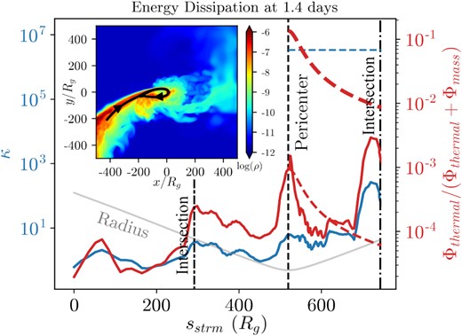
At early times in our aligned TDET0 simulation, the stream heats up at the pericentre and the self-intersection. However, the majority of the entropy generation occurs at the self-intersection, suggesting that the pericentre heating is nearly adiabatic. To see this, we plot the relative amount of heating ψ (equation 18) and a proxy for entropy κ ∝ eentropy against the distance along a streamline sstrm at an early time, 1.34 d. The streamline, depicted in the inset plot, is integrated from the velocity field using a second-order Runge-Kutta method. The location of the pericentre and self-intersections along the streamline are depicted by vertical dashed and dot-dashed lines, respectively. The thin grey line shows the distance between the streamline and the BH. The average entropy of the disc is shown by the blue horizontal dotted line. The thin and thick red lines show an approximation for the relative amount of heating ψ for a thin (h/r = 0.082) and thick (h/r = 1) disc, respectively (equation 21). Note that the returning gas will not necessarily follow the path of the streamline, so sstrm is not a perfect proxy for time. For instance, the entropy sometimes decreases mildly as sstrm increases.
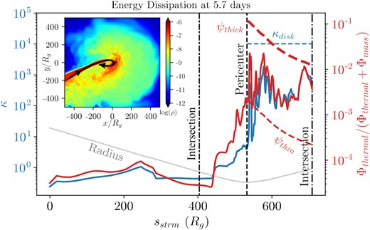
Analogous to Fig. 12, but at a late time of 5.66 d. At late times in our aligned TDET0 simulation, the bulk of the heating and entropy generation occurs at the pericentre radius, suggesting that the pericentre is the most significant source of energy dissipation. The thin and thick red lines show an approximation for the relative amount of heating ψ for a thin (h/r = 0.132) and thick (h/r = 1) disc respectively (equation 21).
Figs 12 and 13 show the early- and late-time dissipation profiles along a streamline, respectively. Although heating and entropy generation occur on similar levels at both times, the dissipation mechanisms are distinct. At early times, there is comparable heating as the stream passes through pericentre and as the outgoing stream reaches the intersection point. However, significant entropy generation occurs only at the self-intersection, suggesting that the heating at pericentre is nearly adiabatic while the heating at self-intersection is irreversible and shock-induced. The nearly adiabatic heating at pericentre implies that the nozzle shock is inefficient at dissipating orbital energy.
At late times, the bulk of the heating and the entropy generation occurs at the pericentre. After the pericentre passage, entropy increases to more than three quarters the entropy of the disc, with the remainder of the entropy generation occurring between the pericentre and self-intersection radii.
The greater value of ψ along the streamline in Fig. 13 compared to Fig. 12 indicates that more heating takes place along the streamline at late times, possibly due to the stream–disc interactions discussed in Section 4.1. However, this does not imply that more heating occurs at late times in the disc as a whole. In particular, we find that the average value of ψ within the disc is greater at time of Fig. 12 than at the time of Fig. 13, suggesting that more relative heating occurs within the disc at early times.
As discussed in Section 3.1, the accretion disc becomes thicker and more massive over time. Therefore, as time progresses, the disc absorbs a greater proportion of the momentum of the outgoing stream, reducing the impact of the self-intersections. When the rotational momentum of the disc surpasses the momentum of the outgoing stream, the outgoing stream disintegrates and the self-intersections stop all together.
In Fig. 14, we plot the rotational mass flux of the disc and the mass fallback rate. The mass fallback rate is a good approximation for the mass flow rate in the outgoing stream; particularly at early times when the incoming and outgoing stream mass flow rates are most similar. At early times, the ratio of the rotational mass flux to the mass fallback rate is less than unity (Fig. 14, top panel). This reflects that the accretion disc mass is small relative to that of the outgoing stream. The ratio of rotational mass flux to mass fallback rate only exceeds unity shortly after the first self-intersection event at 1.5 d. With each self-intersection, the disc grows more substantive until the disc completely intercepts the outgoing stream and self-intersections can no longer occur around 3.7 d in our simulation.
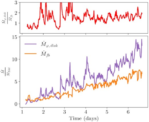
The mass fallback rate and the rotational mass flux in the disc in our aligned TDE simulation. The mass fallback rate is the mass flux in the stream (distinguished by the entropy condition) through the tidal sphere. The rotational mass flux is estimated by azimuthal mass flux of the disc through the surface given by φ = 1.14π, 10 < r < 500, and π/2 − h/r < θ < π/2+h/r. The ratio of rotational mass flux to fallback rate is shown in the top panel. As the disc becomes denser and more massive over the course of the simulation, the rotational mass flux of the disc surpasses the mass fallback rate. Around 3.7 d, the disc completely intercepts the momentum of the outgoing stream and self-intersections can no longer occur.
At early times, the incoming stream heats up before the pericentre passage at the self-intersection point. This is reflected in Fig. 12 by the dramatic increase in ψ in the incoming stream at the intersection point. At the late times, this intersection is too weak to appreciably heat the incoming stream. Instead, the heating before the pericentre passage is caused by the collision between the incoming stream and the dense inner accretion disc. This is reflected in Fig. 13 by the increase in ψ and entropy after the self-intersection point and before the pericentre passage. Together, these results suggest that the self-intersections play a larger role in the energy dissipation at early times in the TDE evolution.
The inclusion of a more realistic equation of state within the debris stream is expected to yield an even higher rate of dissipation due to hydrodynamical shocks (see Guillochon et al. 2014, section 3.3, paragraph 6). Additionally, the inclusion of magnetic fields is expected to yield extra dissipation through the action of magnetorotational instability (MRI; Balbus & Hawley 1991) when the inner and outer stream develop a strong shear in velocity near pericentre.
4.2 Circularization
In the standard TDE picture, the accretion disc circularizes efficiently as shocks dissipate orbital energy, resulting in a nearly axis-symmetric accretion disc with low eccentricity. However, not all TDE discs circularize completely (Piran et al. 2015). Cao et al. (2018) find that the optical emission lines of TDE ASASSN-14li are best modelled by an accretion disc with eccentricity e = 0.97. Furthermore, recent analytical work on TDEs has derived eccentric disc solutions which can produce radiation consistent with the X-ray and optical luminosities of many TDE candidates (Zanazzi & Ogilvie 2020).
Due to the short duration of our simulation, we cannot confirm whether more complete circularization will occur at times after the end of our simulation. One factor that may inhibit circularization is the injection of high-eccentricity material into the disc by the returning debris stream. However, this effect will become negligible when the mass fallback declines to the point where energy and angular momentum input are negligible in analogy to the late-time behaviour of the disc mass in Cannizzo et al. (1990).
Fig. 15 shows a time-averaged streamline plot of the inner part of the disc coloured by eccentricity. The area immediately surrounding the stream contains high-eccentricity material, indicating that the stream continuously transfers its energy and angular momentum into the disc. Away from the stream, disc material orbits at more moderate eccentricities. Looking at snapshots throughout the duration of the simulation, we see a similar distribution of eccentricities in the disc (Fig. 16). Fig. 15 also shows that the eccentricity changes along each streamline, suggesting a continuous transport of energy and angular momentum within the disc itself.
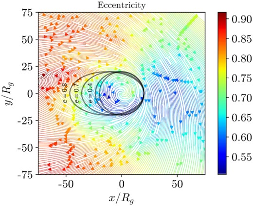
A time-averaged velocity streamline plot of the inner parts of the disc in the equatorial plane coloured by time-averaged eccentricity. Velocity and eccentricity are time-averaged over the simulation’s entire duration, averaged over |θ − π/2| < 0.5, and weighted by rest mass density. The stream is ignored using the entropy condition. The streamlines are integrated using a second-order Runge-Kutta method. Ellipses of various eccentricities are overlaid to provide context for the eccentricity data.
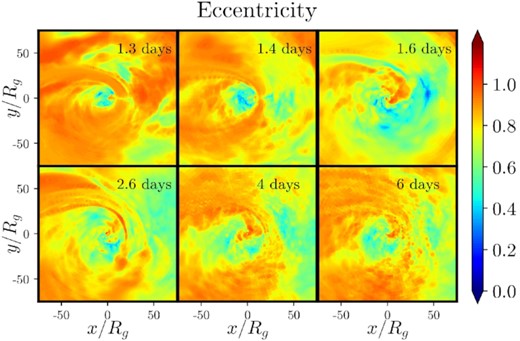
Snapshots of mass-weighted eccentricity in the equatorial plane at various times (see legend) averaged over θ = π/2 ± 0.5. The stream is ignored using the entropy condition. However, there still is an abundance of high-eccentricity material around the stream, suggesting that the stream constantly transfers its energy and angular momentum into the disc.
Eccentricity is not evenly distributed across the different radii in the disc (Fig. 17). In particular, the inner parts of the disc are more circularized than the outer parts. This indicates that circularization is more efficient at smaller radii, possibly because the velocity shear between neighbouring radii is greater. Because eccentricity affects mean φ-velocity (Section 4.4), the uneven eccentricity distribution may contribute to the drop in φ-velocity near the outer edge of the disc in Fig. 6.
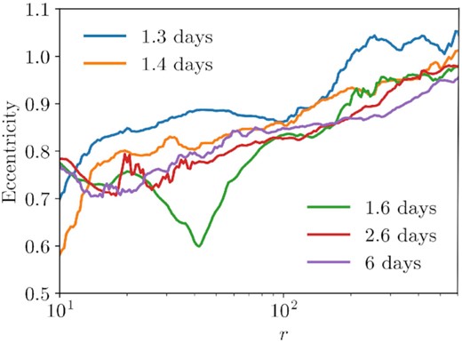
Radial profile of eccentricity at various times (see legend; compare to Fig. 16). Eccentricity is mass-weighted and averaged over spherical shells. The stream is ignored using the entropy condition. Unbound material is ignored using the Bernoulli parameter. Only radii from 10Rg/c to 500Rg/c are shown. Eccentricity is unevenly distributed throughout the disc. In particular, we see greater circularization at smaller radii in the disc.
In Fig. 17, there is a dip in the eccentricity at the self-intersection radius at 1.6 d. This may be a result of the second major self-intersection event, which occurs at 1.47 d, interrupting the incoming stream. This is visible in Fig. 16, where we can see that the effect of the stream on the disc eccentricity is much weaker than at any other time slice shown.
4.3 Accretion and outflow
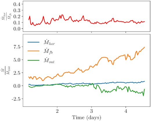
If we assume that ϵ = 0.1, then we find |$\dot{M}_{\rm{Edd}} \simeq 0.022\, {\rm M}_\odot \rm{yr}^{-1}$|. Fig. 18 shows that the mass accretion rate at the BH reaches up to twice the Eddington limit, and the mass fallback rate reaches up to eight times the Eddington limit. This confirms that the TDE in our simulation exhibits the predicted period of super-Eddington accretion. We noted in Section 2.1 that the maximum fallback rates in our simulation are about an order of magnitude lower than the peak fallback rate due to the short duration of our simulation. Therefore, at its peak the accretion rate would be even more super-Eddington than seen in Fig. 18.
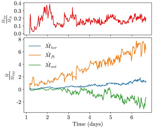
Mass fallback rate, mass accretion rate at the event horizon, mass outflow rate, and the accretion efficiency plotted versus time in our aligned TDET0 simulation. The accretion efficiency settles to around 10 to 20 per cent at t ≳ 4 d. Positive mass fluxes are directed towards the BH. The accretion efficiency is calculated as a ratio of the mass flux at the event horizon to the mass fallback rate. Mass fallback rate is computed within the stream (distinguished by the entropy condition) through the tidal sphere. Mass outflow rate is computed as the unbound mass flux through the tidal radius. Bound matter is ignored using the Bernoulli parameter. All three mass fluxes increase roughly linearly with time, suggesting that the disc mass increases quadratically.
Fig. 19 shows that bound and unbound material accrete on to the BH at increasingly higher rates as the simulation evolves. However, outside of the innermost radii in the disc, more material flows away from the BH than towards the BH. This outward mass flux drives the radial expansion of the disc. The figure also shows that the radial mass fluxes of bound and unbound material are similar throughout the simulation, indicating that a significant fraction of the initially bound material gets unbound. We can loosely estimate this fraction by comparing the outflow rate to the mass flux fallback in Fig. 18. Due to the short duration of our simulation, we compute outflow rates as the mass flux of unbound disc material through the tidal sphere. In a longer simulation, we could compute a more precise outflow rate by computing the mass flux at larger radii and at later times. Fig. 18 shows that the outflow rate is approximately 1/3 of the fallback rate, suggesting that this same fraction of infalling material becomes unbound. However, it is possible that the outflows may be artificially suppressed by the density and pressure floors discussed in Section 3.1, so this may be an underestimate for the fraction of material which becomes unbound in a physical TDE.
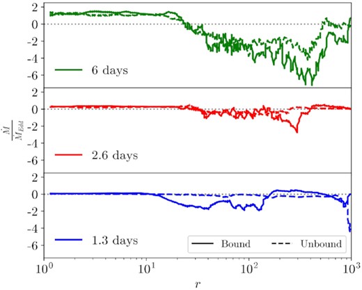
Radial profiles of the mass flux in the disc in units of the Eddington accretion rate. We distinguish between the bound and unbound material at three different times, spread evenly across the duration of the simulation. Positive mass fluxes are directed towards the BH. Bound and unbound material is distinguished using the Bernoulli parameter. The mass flux of bound material is shown in solid lines, and the mass flux of unbound material is shown in dotted lines. The stream is ignored using the entropy condition. The horizontal dotted lines show |$\dot{M}=0$|. Bound and unbound material accrete on to the BH at increasingly higher rates as the simulation progresses.
The rate at which mass is added to the disc is given approximately by subtracting the mass flux outflow and mass accretion rate from the mass flux fallback. Because all three mass fluxes increase linearly with time (Fig. 18), the mass of the disc increases quadratically over the course of our simulation. We verify this by fitting the disc mass to a quadratic time-dependence using the least-squares method. We find that the disc mass in units of grams is given approximately by |$M_{\rm disc}/{\rm M}_\odot = 4.85 \times 10^{-8} t_{\rm days}^2$| with a coefficient of determination R2 = 0.994.
If all accreting material were fully circularized, the accretion efficiency would place a lower limit on the extent of circularization. Then, if no circularization occurred, then the mass accretion rate at the event horizon would vanish, and if the disc circularized completely, then part of the material that falls back would eventually accrete (the rest would fly out as an outflow), giving the lower limit to extent of circularization.
However, we find that a significant fraction of the stellar debris accretes with moderate or high eccentricities, as shown in the left-hand panel of Fig. 20. Here, we plot a time-averaged histogram of the eccentricity of material inside the innermost stable circular orbit, RISCO = 2.04Rg (for prograde orbits in the equatorial plane and our black hole spin value of a = 0.9375; Bardeen, Press & Teukolsky 1972).
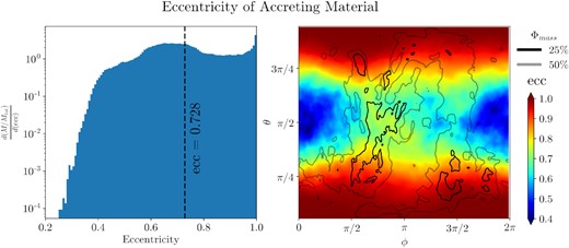
The left-hand panel shows a time-averaged histogram of the eccentricity of material inside RISCO, weighted by rest-mass. Each bin is normalized by total accreting mass and bin width. The mean eccentricity, 〈e〉 ≈ 0.73, is shown by the vertical dashed line. The right-hand panel shows a time averaged colour map of the eccentricity of material inside RISCO, weighted by rest mass. The overlaid grayscale contours outline regions containing 25 and 50 per cent of the total mass flux. Floor material is ignored using an angular momentum condition (|uϕ| > 10−5). The left-hand panel indicates that a significant fraction of material accretes with moderate eccentricities, allowing for a high accretion efficiency without complete circularization. However, from the right-hand panel, we see that highly eccentric material preferentially accretes at high latitudes, except for the material at azimuthal angles just beyond that of the pericentre (see the text for discussion). Most of the low-latitude (disc) accretion occurs at moderate eccentricity.
Eccentric accretion has been found in several earlier works (Shiokawa et al. 2015; Sądowski et al. 2016; Bonnerot & Lu 2020) and may explain the low luminosity and temperature observed in TDE candidates. A more extreme model was proposed by Svirski et al. (2017) in which magnetic stresses transport the angular momentum away from the black hole, driving eccentric accretion. However, this model does not apply to our simulation, which does not include magnetic fields.
There are two ways that material can accrete with moderate or high eccentricities. Gas in the disc may lose angular momentum through, e.g. turbulent viscosity, shocks, or spiral waves, until it plunges into the black hole. This process is analogous to accretion in a quasi-circular accretion disc. Alternatively, gas at high latitudes may get torqued and free fall directly into the black hole, an effect which has been observed in previous works (see fig. 12 of Sądowski et al. 2016). We call the first type of accretion eccentric disc accretion and the second type of accretion ballistic polar accretion.
We can differentiate between these two types of accretion by the latitude at which matter enters the region r < RISCO. We find that highly eccentric material (e > 0.7) preferentially accretes at high latitudes, suggesting that the dominant method of highly eccentric accretion is ballistic polar accretion (Fig. 20). Material accreting at low latitudes generally has more moderate eccentricities (0.4 < e < 0.7), and is thus likely driven by eccentric disc accretion. However, there is a patch of high eccentricity material at low latitudes in the region 2π/3 < ϕ < π, just past the pericentre at an azimuthal angle of ϕ = π/2. Accretion in this region may be due to coherent chunks of the incoming stream that undergo turbulent exchange angular momentum with the disc and accrete directly on to the black hole (see also Fig. 16). The innermost (25 per cent) mass flux contour in Fig. 20 indicates that the majority of accretion occurs in this region.
As we describe in Section 3.1, the debris stream in our aligned TDE simulation collides with itself in five violent self-intersection events that occur approximately 12 h apart and last for roughly 2000Rg/c, or 2.74 h. We apply these results to TDE Swift J1644+57, which exhibits quasi-periodic flaring during the first few days of its initial evolution. Other authors have proposed that this flaring is due to a precessing jet (Stone & Loeb 2012; Tchekhovskoy et al. 2013). However, our simulations show that even without precession, the flaring due to violent self-intersections can explain both the number of flares and their time-scale. Swift J1644+57 is a |$10^5\!-\!10^6\, {\rm M}_{\odot }$| BH, so 1 d corresponds to a time-scale of 5000–50000 Rg/c, similar to the time-scale of the self-intersections in our simulation.
It is unlikely that this flaring is a direct consequence of self-intersection events because the material at the self-intersection point is too optically thick to produce X-rays without adiabatic cooling (Jiang, Guillochon & Loeb 2016). Instead, we propose that the periodicity of the self-intersections leads to a periodicity in the accretion that feeds the jets, an effect that we see in our aligned TDE simulation.
As we discuss in Section 4.2, we can normalize the mass accretion rate at the event horizon by the mass fallback rate for the aligned and tilted simulations. We see quasi-periodic behaviour only in the aligned case (Fig. 18) where violent, periodic self-intersections occur. This behaviour does not perfectly correlate with the major self-intersection events in the simulation, which may be due to the similar time-scale of the self-intersections (∼12 h apart lasting ∼3 each) and the fallback time from the self-intersection point (∼4 h). However, the large fluctuations in accretion rate stop after the last major self-intersection event at 3.7 d.
Sądowski et al. (2016) found a marginally bound torus after self-intersection with some unbound material at high polar angles. They also found periodic behaviour due to the interactions of the outgoing stream with the incoming stream. However, this interaction was not as violent as in our simulation, which may be due to the differences in the orbital properties of the initial star.
4.4 Force balance
In Section 3.1, we show that the φ-velocities in the accretion disc are 76 per cent of the expected φ-velocities in a circularized Keplerian accretion disc. There are two possible explanations for our findings. First, the non-zero eccentricity of the disc decreases the average φ-velocity of the disc relative to a completely circularized disc. Secondly, the disc is internally supported by non-gravitational forces.
As we discuss in Section 4.2, the average eccentricity of the disc at late times is e = 0.88. To determine the effect of this eccentricity on the velocity distribution, we set up artificial velocity fields with constant eccentricities of 0 and 0.88 using a method described in Appendix A3. For each velocity field, we compute the radial profile of φ-velocity with equation (11), where the density weight is determined as a function of radius by the power-law relationship depicted in Fig. 6. On average, we find that the φ-velocities in the eccentric disc are 93.8 per cent of the φ-velocities in the circularized disc. Therefore, the φ-velocities in our accretion disc are at most |$76{{\ \rm per\ cent}} / 0.938 = 81{{\ \rm per\ cent}}$| of the φ-velocities in a Keplerian accretion disc at the same eccentricity. Therefore, the disc must also be externally supported by non-gravitational forces.
A time-averaged radial profile of the pressure gradient force density normalized by the Keplerian force density. Within the disc, we see that pressure gradient forces are a significant fraction of the Keplerian force, accounting for the sub-Keplerian φ-velocity distribution that we find in Fig. 6. Pressure is averaged over spherical shells and mass-weighted. Time averages are over the simulation’s full duration. The stream is ignored using the entropy condition. We apply a smoothing function to the data to improve readability.
4.5 Comparison to disc models
4.5.1 Comparison to ZEBRA model
We compare the properties of the post-intersection accretion flow in our simulation with those predicted by the ZEro-BeRnoulli Accretion (ZEBRA) model proposed by Coughlin & Begelman (2014). The key assumptions of the ZEBRA model are that
the Bernoulli parameter b is zero everywhere,
the potential is Newtonian,
the magnetic energy density is not sufficient to destabilize the disc with respect to the Høiland criteria.
Coughlin & Begelman (2014) show that assumption (i) ensures that the disc is gyrentropic; that is, surfaces of constant entropy, angular momentum, and Bernoulli parameter coincide. From assumption (ii), Newton’s law, and the Bernoulli equation, Blandford & Begelman (2004) derive self-similar solutions for gyrentropic discs with an arbitrary Bernoulli parameter. The ZEBRA solutions are a special case when the Bernoulli parameter is zero everywhere.
Assumption (iii) trivially holds in our simulations due to the absence of magnetic fields. We show that assumption (i) holds in Fig. 2, which depicts a histogram of the Bernoulli parameter weighted by mass in the initial conditions. We calculate that the average mass-weighted Bernoulli parameter in the initial conditions is 3.6 × 10 − 5. The Bernoulli parameter in the disc is larger than this initial parameter because only the most bound debris reaches the black hole over the duration of our simulation. However, even at late times, the Bernoulli parameter is smaller than the gravitational binding energy within the disc. At 5.7 d into the simulation, the average mass-weighted Bernoulli parameter is approximately 1.5 × 10⁻³, or 38 per cent of the binding energy in the disc at a characteristic radius r0 = 259Rg determined by the mass-weighted mean radial coordinate of the disc.
ρ ∝ r−q,
p ∝ r−q − 1,
1/2 < q < 3,
l ∝ sin 2θ,
ρ ∝ (sin 2θ)α,
p ∝ (sin 2θ)α,
Equation (31).
We compare the ZEBRA model predictions to the radial and polar profiles of our simulated disc (Figs 6 and 7). (a) and (b) imply that density and pressure depend on r as a power law and (e) and (f) imply that density and pressure depend on θ as a power law of sin 2θ. These predicted dependencies provide a reasonable fit for our data within the boundaries of the disc (Tables B1 and B2). Our fitted power-law exponents for the radial profiles density and pressure differ by 1.22, which nearly matches the difference of 1.0 predicted by (a) and (b). In the model of Coughlin & Begelman (2014), the power-law index q can be constrained by the mass inflow rate and prescribed disc physics (e.g. the fact that angular momentum is efficiently transported in the disc), but in general it is expected to be on the order of ∼1 − 2 (see fig. 8 of Coughlin & Begelman 2014 and fig. 4 of Wu et al. 2018), which is exactly what we see in our simulation.
Curve-fitting results for the radial profiles of mass density, pressure, and φ-velocity from 20–250 Rg shown in Fig. 6, including the power-law parameters (axb) and their relative standard deviation errors. The exponent for φ-velocity is fixed at -0.5.
| Variable | a | σa/μa | b | σb/μb |
|---|---|---|---|---|
| ρ | 4.13E-7 | 4.71 per cent | −1.10 | 1.26 per cent |
| Pressure | 2.54E-7 | 7.37 per cent | −2.32 | 1.00 per cent |
| φ-velocity | 0.759 | 1.64 per cent |
| Variable | a | σa/μa | b | σb/μb |
|---|---|---|---|---|
| ρ | 4.13E-7 | 4.71 per cent | −1.10 | 1.26 per cent |
| Pressure | 2.54E-7 | 7.37 per cent | −2.32 | 1.00 per cent |
| φ-velocity | 0.759 | 1.64 per cent |
Curve-fitting results for the tilted TDE radial profiles of mass density, pressure, and φ-velocity from 20–250 Rg shown in Fig. 10, including the power-law parameters (axb) and their relative standard deviation errors. The exponent for φ-velocity is fixed at -0.5.
| Variable | a | σa/μa | b | σb/μb |
|---|---|---|---|---|
| ρ | 5.19E-7 | 1.73 per cent | −1.34 | 0.397 per cent |
| Pressure | 2.91E-7 | 6.75 per cent | −2.62 | 0.840 per cent |
| φ-velocity | 0.593 | 2.17 per cent |
| Variable | a | σa/μa | b | σb/μb |
|---|---|---|---|---|
| ρ | 5.19E-7 | 1.73 per cent | −1.34 | 0.397 per cent |
| Pressure | 2.91E-7 | 6.75 per cent | −2.62 | 0.840 per cent |
| φ-velocity | 0.593 | 2.17 per cent |
However, the alpha parameter does not match its predicted value from the ZEBRA model. The power-law exponent for density indicates that q ∼ 1. Therefore, α ∼ 0.5 by equation (31). Instead, we find values for α of unity and 12 from pressure and density, respectively. In addition, l2 is proportional to (sin 2θ)2.2 rather than sin 2θ. These discrepancies indicate that the disc must be thinner than predicted by the ZEBRA model.
The ZEBRA model predicts that the specific angular momentum of the disc must be at least 76 per cent of the Keplerian value with our assumption of a polytropic index of 5/3 (Coughlin & Begelman 2014). Coincidentally, we find that the φ-velocities in the disc are 76 per cent of the Keplerian values for circular orbits. As we discuss in Section 4.4, the non-zero eccentricity of our disc automatically decreases the φ-velocities in the disc relative to the Keplerian velocity. Adjusting for this effect, the φ-velocities in the disc are 81 per cent of the Keplerian values.
As we mention in Section 3.1, the internal energy density and mass density floors at 2.27 × 10⁻¹² may artificially decrease the radial and vertical extent of the disc by providing external pressure support. Therefore, our results at radii within the disc boundaries (≲ 500Rg) are more reliable than at larger distances. Without the floors, it is possible that the power-law curves for density and pressure in Figs 6 and 10 would continue past 500Rg. This additional pressure confinement may also be responsible for the flattening of the disc as compared to the ZEBRA model. Because the floors are non-rotating, the external pressure could decrease the angular momentum of material at the edges of the disc, possibly leading to artificially efficient accretion.
4.5.2 Bonnerot and Lu model
Recently, Bonnerot & Lu (2020) performed a TDE simulation with a realistic stellar trajectory and mass ratio. They found that self-intersections launch outflows. These outflows undergo extensive ‘secondary shocks’ that ultimately result in the formation of an accretion disc. This contrasts with our results, in which the formation and circularization of the accretion disc results primarily from stream–disc interactions near pericentre (Section 4.1). Even when violent self-intersections do not occur, as in model TDET30, an accretion disc still forms.
Bonnerot & Lu (2020) overcame the numerical challenges of simulating a TDE with a realistic stellar trajectory and mass ratio by using a non-spinning BH and incorporating the local simulation of Lu & Bonnerot (2019) into their initial conditions to describe the outflows produced by self-intersection shocks. However, that local simulation includes assumptions that maximize the impact of the self-intersection shocks.
Lu & Bonnerot (2020) perform their simulation in a special inertial frame, which they refer to as the simulation box (SB) frame, in which the incoming and outgoing streams collide head-on. The frame is related to the lab frame by a boost to the comoving frame of a local stationary observer at the self-intersection radius followed by a boost to a frame where the φ-velocity of the outgoing stream vanishes. This technique relies on three assumptions.
First, it requires that the incoming and outgoing streams have equal (φ-velocities, aspect ratios) or precisely opposite (radial velocities) properties at the point of self-intersection. However, significant pericentre dissipation, Lense–Thirring frame dragging, or hydrodynamic instabilities at the boundary of the stream and the disc could cause the outgoing stream to have a lower density and velocity and a different trajectory relative to the incoming stream, decreasing the violence of the self-intersections.
Secondly, the incoming and outgoing streams are only completely parallel in the SB frame at the intersection point. As the radial distance from the self-intersection point increases, the head-on gas trajectories used in Lu & Bonnerot (2019) diverge from the physical trajectories. Therefore, the approach is only accurate in the case that there are minimal interactions between pre- and post-intersection material and, e.g. the accretion disc. By ignoring these interactions, the head-on approach increases the relative importance of the self-intersections in the overall TDE evolution.
Thirdly, the Lu & Bonnerot (2019) simulation uses 2D cylindrical coordinates, implicitly assuming axisymmetry of the colliding streams. This 2D approach also cannot fully capture 3D fluid instabilities and turbulence inherent in the violent interaction.
Many of the novel effects observed by Bonnerot & Lu (2020) are tied to the strong outflows sourced at the self-intersection point: for instance, the formation of a retrograde accretion disc with respect to the star’s initial orbital angular momentum is due to the preferential loss of prograde debris in the self-intersection outflows. In our simulations, stream–disc interactions near pericentre rapidly become the primary locus of energy dissipation and efficiently suppress the return of coherent outgoing streams to the self-intersection site. This behaviour is difficult to reconcile with local mass injection schemes near the self-intersection radius.
One source of the discrepancy between our work and that of Bonnerot & Lu (2020) may be the high-β encounter analyzed here, which causes the outgoing stream to significantly expand after the pericentre passage due to differential precession (Section 3.1). For a more standard TDE with β ≈ 1, the approach of Bonnerot & Lu (2020) may become more accurate. It is also possible that increasing the resolution across the vertical extent of the stream in our simulation would result in stronger nozzle shocks. We leave it to future work to apply our methods to less deeply penetrating TDEs.
4.6 Analysis of the tilted TDE simulation, model TDET30
Fig. 22 shows that the accretion efficiency of the tilted TDE is only slightly less than the aligned TDE, hovering from 10 to 15 per cent. Just like the aligned scenario, all three mass fluxes increase roughly linearly in time, implying a quadratically increasing disc mass.
Analogous to Fig. 18, but for the tilted TDE simulation, model TDET30. The accretion efficiency is similar to that of the aligned run.
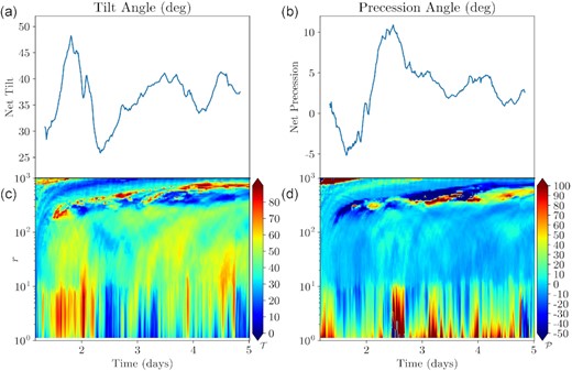
The tilt angle |$\mathcal {T}$| and precession angle |$\mathcal {P}$| of the tilted disc over time in our titled TDE simulation TDET30. Panels (a) and (b) depict the tilt and precession angles calculated from the net angular momentum of the disc for material r < 500Rg. Panels (c) and (d) depict the tilt and precession angles calculated from the net angular momentum of the disc material at the radius indicated on the y-axis. Both tilt and precession angles are continuous within the range of radii in the disc outside of stream’s pericentre (10Rg ≲ r ≲ 200Rg at the beginning of the simulation and 10Rg ≲ r ≲ 400Rg at the end of the simulation), indicating that there is no disc-tearing. Below 10Rg, tilt and precession angles fluctuate rapidly due to stream–disc interactions at pericentre. We do not observe significant precession of the disc in the duration of the simulation. It is possible that disc precession at small radii is inhibited by the constant injection of stream material in the orbital plane of the star.
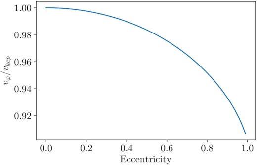
The ratio of φ-velocity to circular Keplerian velocity for orbits of various eccentricities. We compute φ-velocity by setting up artificial velocity fields in the equatorial plane with a constant eccentricity. Then, we average φ-velocity over radius using a mass weight determined by the power law of best fit for the mass density radial profile in the aligned TDE simulation.
At the times well before peak fallback time considered in our simulation, the fallback rate of the stellar debris increases linearly with time (Fig. 22). Therefore, the debris stream accounts for a significant proportion of the total angular momentum budget. By summing the components of Newtonian angular momentum in the region r < 500Rg, we estimate that the net angular momentum of the stream in this region is approximately 7 per cent of the net angular momentum of the disc at late times.
Previous GRMHD simulations of tilted accretion discs have shown disc tearing, where the accretion disc occupies separate planes over different ranges in radii (Liska et al. 2021). disc tearing occurs when the torque exerted on the disc by differing rates of Lense–Thirring precession at different radii surpasses the viscous forces holding the disc together. In particular, the inner part of the disc may become aligned with the equatorial plane of the BH, a phenomenon known as Bardeen–Peterson alignment. The continuity of the tilt and precession angles over the range of radii in the disc (Fig. 23) suggests that the disc remains intact. Similarly to precession, disc tearing and Bardeen–Peterson alignment may be inhibited by the contribution of angular momentum from the stream.
At times well after the end of our simulation, the mass accretion rate will drop below the Eddington limit. Therefore, the disc may cool and begin precessesing and/or tearing. Since this simulation was not run for multiple viscous times of the accretion disc, the presence of precession in tilted TDEs remains an open question.
5 CONCLUSIONS
In this work, we simulate a tidal disruption of a Sun-like star by a supermassive BH for a realistically large mass ratio (Q = 106) and for a realistic stellar orbit (e0 ≈ 1). We simulate the initial disruption in post-Newtonian SPH and migrate to full GRHD as the debris stream approaches the BH. We also present the first simulation of a tilted TDE in GRHD (Section 6). Our use of realistic parameters poses a number of challenges. A high mass ratio leads to a thin stellar debris stream that is difficult to resolve. We accommodate this difficulty using two levels of AMR. A parabolic stellar trajectory necessitates a large range of temporal and spatial scales. As the initial eccentricity of the star increases, the fallback time of the stellar debris and the apocentre of the debris stream orbit grow. The unprecedented efficiency of h-amr due to GPU-acceleration and AMR allows us to cover the necessary range of scales to simulate the earliest stages of accretion disc formation.
We find that the TDE naturally and efficiently forms an accretion disc, although the high-eccentricity material constantly supplied by the stream inhibits circularization. The accretion efficiency fluctuates between 10 and 20 per cent over the duration of our simulation (Fig. 18). We also find that a significant fraction of material accretes at moderate eccentricities (0.4 < e < 0.7), with highly eccentric material (e > 0.7) preferentially accreted at high latitudes (Fig. 20).
During the post-disruption phase of our aligned TDE simulation, the debris stream undergoes a series of violent self-intersection events in which the incoming and outgoing streams collide. We propose that these self-intersections are the phenomena responsible for the early-time flaring of TDE Swift J1644+57 and other TDEs. The self-intersections account for both the number of flares and their time-scale.
At early times (i.e. during the first 3 d of the simulation), self-intersections play a crucial role in orbital energy dissipation. At late times, the newly formed accretion disc completely intercepts the outgoing stream, causing the violent self-intersection events to cease. As a result, stream–disc interactions near pericentre are the dominant dissipation mechanism. These interactions raise the entropy of the debris stream three quarters of the way to the final entropy of the accretion disc (Fig. 13). Consequently, thermal energy flux dominates over mass energy flux in the debris stream post-pericentre compared to before the pericentre passage.
We find that the newborn disc exhibits super-Eddington accretion. The radial and polar dependencies of density and pressure within the disc closely reflect the self-similar solutions proposed by Coughlin & Begelman (2014) in the ZEBRA model. Non-zero eccentricity has a small effect on the deviation from Keplerian velocities in the disc, and the more prominent effects are from thermal pressure gradient forces (Fig. 21). The thermal energy generated by accretion heats up the inner part of the disc. The temperature distribution through the disc creates a thermal pressure gradient force that supports the disc against gravity, leading to a sub-Keplerian velocity distribution.
For a TDE with a 30 deg BH-spin–stellar-orbit misalignment angle, we find that nodal precession causes the incoming and outgoing streams to intersect off-centre (Fig. 9). This ejects gas from the outgoing stream on to orbits with larger tilt angles and results in less violent self-intersections. However, an accretion disc still forms with a similar accreted fraction of the material to the aligned case.
The largest drawback of our simulation is its short duration, of about one week, which allows only the small fraction of the stellar debris with specific energy well outside the frozen-in approximation to accrete on to the BH (Section 2.1). However, these early stages of TDE disc formation are crucial because they capture the initial disc formation and the emergence of the orbital energy dissipation mechanism. Our results suggest that disc formation in TDEs may be a runaway process; once sufficient mass has partially circularized at small radii, stream–disc interactions become the dominant dissipation mechanism, further growing the (initially eccentric) accretion disc. Clearly, the late-time evolution of TDE discs requires further study, particularly as the fallback rate approaches its peak and deviates from linear growth.
As discussed in Section 2.3, it is possible that we under resolve pressure gradients within the stream. This will be corrected in future simulations by including additional levels of AMR. In future work, we plan to study how TDE accretion disc formation is affected by the magnetic field of the disrupted star. This will allow us to model the MRI of the disc. We also plan to incorporate a variable polytropic index based on the equation of state used by Shiokawa et al. (2015) to more accurately model the thermodynamics of the disc. Finally, we will either use the pseudo-Newtonian potential from Tejeda & Rosswog (2013) in our initial SPH simulation or we will model the entire disruption in full general relativity.
SUPPORTING INFORMATION
Please note: Oxford University Press is not responsible for the content or functionality of any supporting materials supplied by the authors. Any queries (other than missing material) should be directed to the corresponding author for the article.
ACKNOWLEDGEMENTS
We thank the anonymous referee for their detailed feedback which has greatly enhanced the clarity of this work. In particular, we thank the referee for the suggestion to analyse the eccentricity of accreting material in more detail. This research was made possible by National Science Foundation (NSF) Petascale Computing Resource Allocation awards no. 1615281 and OAC-1811605 as part of the Blue Waters sustained-petascale computing project, which is supported by the NSF (awards OCI-0725070 and ACI-1238993) and the state of Illinois. Blue Waters is a joint effort of the University of Illinois at Urbana-Champaign and its National Centre for Supercomputing Applications. Additional computer time was provided by the Innovative and Novel Computational Impact on Theory and Experiment (INCITE) program under award PHY129. This research used resources of the Oak Ridge Leadership Computing Facility, which is a Department of Energy Office of Science User Facility supported under Contract DE-AC05-00OR22725.
Eric Coughlin ackowledges support from the National Aeronautics and Space Administration (NASA) through the Hubble Fellowship Program, grant #HST-HF2-51433.001-A awarded by the Space Telescope Science Institute, which is operated by the Association of Universities for Research in Astronomy, Incorporated, under NASA contract NAS5-26555, and NSF grant AST-2006684. Alexander Tchekhovskoy is supported by the National Science Foundation grants AST-1815304 and AST-1911080. Nicholas Stone received financial support from NASA, through both Einstein Postdoctoral Fellowship Award Number PF5-160145 and the NASA Astrophysics Theory Research Program (Grant NNX17AK43G; Principal Investigator B. Metzger). He also received support from the Israel Science Foundation (Individual Research Grant 2565/19). Matthew Liska was supported by the John Harvard Distinguished Science Fellowship and the Institute for Theory and Computation Fellowship.
Our simulation, post-processing, and analysis relied on tools from the scipy and numpy Python libraries (Jones et al. 2001; Oliphant 2006). Our 2D and 3D visualizations relied on the matplotlib Python Library and the visit visualization software, respectively (Hunter 2007; Childs et al. 2012).
DATA AVAILABILITY
Movies and 3D renderings are available at MNRAS online and on YouTube. Simulation data are available upon request from Alexander Tchekhovskoy at [email protected].
Footnotes
The tidal tensor implied by the Einstein potential produces a moderately different tidal shear than the exact general relativistic value. However, the general relativistic corrections to the Newtonian tidal shear (either exact or from equation 1) are only |$\mathcal {O}(5{{\ \rm per\ cent}})$| at the tidal radius where the star is disrupted, and ballistic motion sets in.
REFERENCES
APPENDIX A: DERIVATIONS
In this appendix, we provide several derivations used in our analysis which did not fit into the main body of the text.
A1 Bernoulli parameter
A2 Equatorial geodesics
A3 Artificial velocity fields
A4 Analytical self-intersection radius
APPENDIX B: CURVE FITTING DATA
In this appendix, we provide the curve fitting data for Figs 6 and 10 in Tables B1 and B2, respectively.
APPENDIX C: TILTING ALGORITHM
In this appendix, we describe the tilting algorithm used in our analysis of model TDET30. For our analysis of the tilted TDE, we untilt the data so that the orbital plane of the star lies in the equatorial plane. For each point on our original spherical grid, we convert to Cartesian coordinates and multiply by the rotation matrix |$\rm {R}_y(\pi /6)$|. Then, we use a third-order spline method to interpolate our data to each point on the rotated grid.
In Fig. C1, we test our tilting algorithm by tilting and untilting one time slice. While the edges of the stream lose some of their definition, the overall structure of the system remains intact.
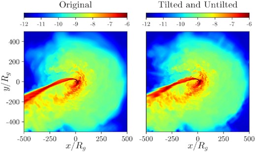
Contour plots of the log of rest mass density in the equatorial plane at 5.7 d. The left-hand panel shows the unaltered data and the right-hand panel shows the data after two applications of the tilting algorithm at angles of π/6 and −π/6.
Author notes
John Harvard Distinguished Science and ITC Fellow
