


ABSTRACT
We present spectral and temporal properties of all the thermonuclear X-ray bursts observed from Aql X-1 by the Neutron Star Interior and Composition Explorer (NICER) between 2017 July and 2021 April. This is the first systematic investigation of a large sample of type I X-ray bursts from Aql X-1 with improved sensitivity at low energies. We detect 22 X-ray bursts including two short recurrence burst events in which the separation was only 451 s and 496 s. We perform time resolved spectroscopy of the bursts using the fixed and scaled background (fa method) approaches. We show that the use of a scaling factor to the pre-burst emission is the statistically preferred model in about 68 per cent of all the spectra compared to the fixed background approach. Typically the fa values are clustered around 1–3, but can reach up to 11 in a burst where photospheric radius expansion is observed. Such fa values indicate a very significant increase in the pre-burst emission especially at around the peak flux moments of the bursts. We show that the use of the fa factor alters the best-fitting spectral parameters of the burst emission. Finally, we employed a reflection model instead of scaling the pre-burst emission. We show that reflection models also do fit the spectra and improve the goodness of the fits. In all cases, we see that the disc is highly ionized by the burst emission and the fraction of the reprocessed emission to the incident burst flux is typically clustered around 20 per cent.
1 INTRODUCTION
Thermonuclear (type I) X-ray bursts are caused by the unstable ignition of H/He deposited on the surface of a neutron star in a low-mass X-ray binary (e.g. Truemper, Lewin & Brinkmann 1986; Lewin, van Paradijs & Taam 1993; Bildsten 1998; Strohmayer & Bildsten 2006; Galloway & Keek 2021). When the gas is accreted from a low-mass companion (≲1 M⊙), it accumulates on the surface of the neutron star where it is hydrostatically compressed and heated, the temperature and pressure increases and eventually a thermonuclear explosion can be triggered (Fujimoto, Hanawa & Miyaji 1981; Narayan & Heyl 2003). These events are observed in X-rays as sudden increases in intensity reaching up to a factor of ten to a hundred times the persistent level (Strohmayer & Bildsten 2006; Galloway et al. 2008). Typically, the rise times of bursts can be within 1–10 s, while the bursts themselves can last from a few tens of seconds to several minutes. The total energy output of a burst can be ≈1039−1040 erg (e.g. Galloway et al. 2020). The intensity produced in thermonuclear bursts can have an effect on the surrounding accretion flow (Degenaar et al. 2018), which consists of an accretion disc and a hot electron corona, allowing the bursts to affect the dynamics of the accretion process.
High time and moderate energy resolution observations of thermonuclear X-ray bursts could only be systematically performed with the launch of the Rossi X-Ray Timing Explorer (RXTE) Proportional Counter Array (PCA) in the 2.5–25.0 keV band (see e.g. Taam, Chen & Swank 1997; Galloway et al. 2008, 2020; Chen et al. 2013; in’t Zand et al. 2014; Bilous & Watts 2019). Generally, using a single blackbody component fits X-ray burst spectra well in addition to a constant persistent component (Galloway et al. 2008), especially during the cooling tails of bursts (Güver, Psaltis & Özel 2012a). The persistent component defines the X-ray emission from accretion processes, as measured before and assumed not to change during the burst. Considering a large sample of observations with RXTE/PCA, burst spectra are found to have deviations from this simple blackbody model. Worpel, Galloway & Price (2013, 2015) characterized the deviation from a pure blackbody model using a constant factor to scale the pre-burst emission that is allowed to vary through a given burst. The so-called fa method basically allows the pre-burst emission to vary during the burst to obtain a better fit to the observed data. It was found that allowing the pre-burst emission to vary significantly improves the fits, especially during the bursts where photospheric radius expansion (PRE) is observed and most obviously at around the peak flux times. This variation in the normalization of the pre-burst spectrum is attributed to an increase in the mass accretion rate likely due to Poynting-Robertson drag (Robertson 1937; Walker & Meszaros 1989; Walker 1992). This interpretation is supported by recent simulations (Fragile et al. 2018; Fragile, Ballantyne & Blankenship 2020). However, the fact that the fa parameter is only a multiplication factor to the persistent emission and does not allow for a change in the spectral shape prevents the method from helping understand what really varies within the pre-burst emission.
Systematic studies of the effects of X-ray bursts to their environment have mostly been limited to observations of superbursts (≳1000 s), which happen rarely (Ballantyne & Strohmayer 2004; Keek et al. 2014). These bursts are thought to be powered by the unstable combustion of deeper layers containing helium and carbon, instead of the hydrogen and/or helium expected from a normal type I X-ray burst (in’t Zand 2017). The fact that superbursts are much longer allows for higher integration times for X-ray spectroscopic studies, which allows collecting higher quality spectra than a normal typical burst. Detailed spectral analyses of superbursts revealed the presence of a reflection component of the burst emission from the surface of the neutron star off of the accretion disc (Ballantyne & Strohmayer 2004). The reflection spectrum depends on the composition of the reflective material (see for 4U 1820-30 Ballantyne 2004) as well as the properties of the burst.
NICER combines the sensitivity in the soft X-rays (0.2–12 keV) with large effective area at around 1 keV (Gendreau, Arzoumanian & Okajima 2012; Gendreau et al. 2016; Gendreau, Arzoumanian & NICER Team 2017) together with good energy resolution, which provides an exciting opportunity to study burst–disc interactions in a much more systematic manner. Taking advantage of the soft X-ray sensitivity of NICER, Keek et al. (2018a,b) reported the detection of a strong soft excess in bursts from Aql X-1 and 4U 1820-30. In both cases, application of the fa factor was shown to improve the goodness of the fits to the data with fa values reaching up to 2.5 and 10 for Aql X-1 and 4U 1820-30, respectively. In agreement with Worpel et al. (2013), Keek et al. (2018a,b) found that the existence and strength of PRE appears to drive the significance of the soft excess. Similarly, for Swift J1858.6 − 081 (Buisson et al. 2020) and for MAXI J1807 + 132 (Albayati et al. 2021) application of the fa method improved the fits, although in some cases adding a second blackbody component also improved the fits (Buisson et al. 2020) and may even be preferred as for SAX J1808.4 − 3658 (Bult et al. 2019). On the other hand, for XTE J1739 − 285 (Bult et al. 2021a) and 4U 1608 − 52 (Güver et al. 2021) no statistically significant deviation from a blackbody model has been reported. In both cases, the hydrogen column density in the line of sight is significantly larger, which may be affecting the detection of the soft excess.
As a follow-up to these studies, we here present a spectral and temporal analysis of all the bursts observed with NICERfrom Aql X-1 between July 2017 and April 2021. Our goal is to report the X-ray bursts detected with NICER and systematically study the soft excess that has been reported to be observed from this source before (Keek et al. 2018a). Aql X-1 is one of the ideal sources for such studies given the relatively low hydrogen column density in the line of sight and the fact that the source frequently shows outbursts. Aql X-1 was discovered in 1965 by Friedman, Byram & Chubb (1967). The source is transient, showing frequent, roughly one per year outbursts (Güngör, Güver & Ekşi 2014). The system has an orbital period of 18.9 hr (Chevalier & Ilovaisky 1991). Intermittent pulsations (Casella et al. 2008) and burst oscillations (Zhang et al. 1998; Galloway et al. 2008, 2020; Bilous & Watts 2019) at around 549 Hz have been observed, indicating a fast rotating neutron star in the system. Utilizing phase-resolved near-IR spectroscopic observations, the spectral type of the companion is estimated as K4 and the distance and orbital inclination of the system was found to be 6 ± 2 kpc and between 36° and 47°, respectively (Mata Sánchez et al. 2017). Also, the X-ray reflection modelling of the persistent emission gives an inclination of i = (36 ± 2)° (King et al. 2016; Ludlam et al. 2017). In good agreement with these results, the distance of this source is calculated as d = 5.55 ± 3.57 kpc using the parallax measurement in the recently published Gaia EDR3 catalogue (Gaia Collaboration et al. 2021). A total of 96 X-ray bursts have been reported from Aql X-1 in the MINBAR catalogue (Galloway et al. 2020), implying a burst rate of 0.1 bursts per hour, which is calculated using the available exposure time while the source is active.
2 OBSERVATIONS AND DATA ANALYSIS
Starting from 2017 June 20, NICER observed Aql X-1 for a total of 620 ks with 134 observations. We used all of the observational data of Aql X-1 from NICER, publicly available through the High-Energy Astrophysics Science Archive Research Centre (HEASARC).1 The ObsIDs used in this study cover the following ranges 0050340104-109, 1050340101-125, 2050340101-129, 3050340101-159, and 4050340101-121. Note that ObsIDs starting with a zero were collected during instrument validation and are not publicly available through HEASARC. Applying the standard filtering criteria results in a total clean exposure time of 347 ks, using HEASOFT v.6.27.2, NICERDAS v7a, and the calibration files as of 2020/07/27. We applied barycentric correction to the event files using the source coordinates2 (J2000) RA |$19^{\rm h}11^{\rm m}16{_{.}^{\rm s}}05$| Dec. |$+00{^\circ }35^{\prime}05{_{.}^{\prime\prime}}8$| and JPLEPH.430 ephemerides (Folkner et al. 2014).
Fig. 1 shows the long-term light curve of Aql X-1 as observed by MAXI in the 2–20 keV band during NICER observations. Individual panels show the time intervals when a NICER observation was performed. It can be seen that NICER observations are typically clustered around outbursts of the source. We also generated a hardness intensity diagram of the source based on all of the NICER observations used here. For this purpose, we generated 0.5–10, 2.0–3.8, and 3.8–6.8 keV light curves of all the clean event files with a time resolution of 128 s and computed the hardness ratio by dividing the count rates in the 3.8–6.8 keV by the count rates in the 2–3.8 keV band. The resulting hardness intensity diagram is shown in Fig. 2.
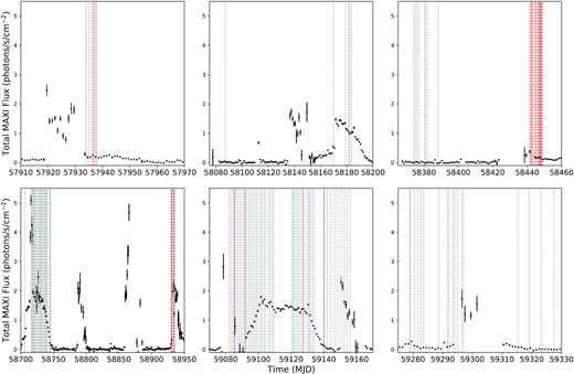
Long term light curve of Aql X-1 as observed by MAXI in the 2–20.0 keV band. The panels show different time intervals when NICER observed the source. The MAXI data is shown with black dots, the grey vertical dashed lines indicate the NICER observation times. The red dashed lines show the times when a thermonuclear X-ray burst is detected. Note that some bursts which occurred with short recurrence are not discernible in the figure.
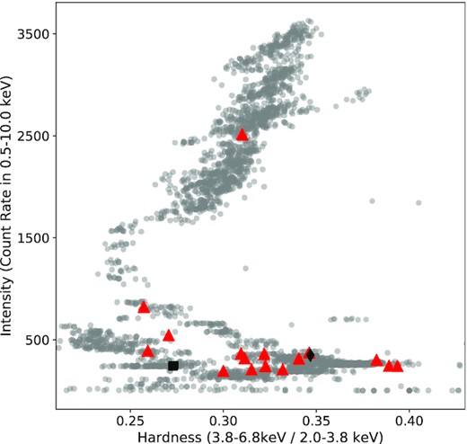
Hardness–intensity diagram extracted from all NICER observations of Aql X-1. Hardness ratio is defined as the ratio of the count rate in the 3.8–6.8 and 2.0–3.8 keV bands. The locations of the detected X-ray bursts are indicated by red triangles. Also in black diamond and square, we show the locations of the short recurrence bursts 15–16 and 21–22, respectively.
We searched for thermonuclear X-ray bursts within all of the unfiltered data and found 22 such events. Some of the basic properties of these bursts are given in Table 1 and 0.5–10 keV light curves are given in Figs A1–A3. We also show the locations of the bursts in the hardness-intensity diagram using data obtained just prior to each burst (see Fig. 2). Note that the time burst 12 occurred is filtered out with the standard filtering criteria, we therefore used unfiltered events for this burst.
Some characteristic properties of all the detected with NICER thermonuclear X-ray bursts from Aql X-1. Parameters are derived from 0.5 to 10.0 keV light curves with a time resolution of 0.5 s, therefore the uncertainties in the rise and decay times are 0.5 s.
| Burst no. | MJD (TDB) | OBSID | Peak ratea | Pre-burst rateb | Rise time | Decay e-folding time |
|---|---|---|---|---|---|---|
| (counts s−1) | (counts s−1) | (s) | (s) | |||
| 1 | 57936.584843 | 0050340108 | 1750 ± 60 | 226 ± 7 | 7.0 | 11.5 |
| 2 | 57937.615500 | 0050340109 | 2620 ± 80 | 272 ± 3 | 3.0 | 17.5 |
| 3 | 58441.896973 | 1050340117 | 3550 ± 90 | 845 ± 3 | 4.5 | 13.5 |
| 4 | 58442.801000 | 1050340118 | 3490 ± 90 | 571 ± 3 | 5.5 | 9.5 |
| 5 | 58442.932044 | 1050340118 | 3300 ± 90 | 581 ± 3 | 4.5 | 14.0 |
| 6 | 58444.845108 | 1050340120 | 2780 ± 80 | 396 ± 2 | 6.0 | 21.0 |
| 7 | 58444.978103 | 1050340120 | 2700 ± 80 | 386 ± 3 | 4.5 | 22.0 |
| 8 | 58446.319741 | 1050340122 | 3250 ± 80 | 356 ± 2 | 3.5 | 15.5 |
| 9 | 58447.182637 | 1050340123 | 3030 ± 80 | 283 ± 2 | 3.0 | –c |
| 10 | 58447.686326 | 1050340123 | 2780 ± 90 | 233 ± 2 | 7.8 | 14.5 |
| 11 | 58447.949824 | 1050340123 | 2830 ± 90 | 231 ± 2 | 6.0 | 17.0 |
| 12 | 58448.526803 | 1050340124 | 2780 ± 90 | 216 ± 2 | 6.5 | 18.0 |
| 13 | 58930.162945 | 3050340101 | 2720 ± 80 | 325 ± 3 | 5.5 | 21.5 |
| 14 | 58930.735030 | 3050340101 | 2640 ± 80 | 349 ± 3 | 9.5 | 23.0 |
| 15 | 58934.487522 | 3050340105 | 2760 ± 80 | 367 ± 3 | 3.5 | 23.5 |
| 16 | 58934.493274 | 3050340105 | 1450 ± 60 | 369 ± 3 | 9.0 | 10.5 |
| 17 | 58934.807525 | 3050340105 | 2730 ± 80 | 387 ± 3 | 8.0 | 17.0 |
| 18 | 59085.311252 | 3050340111 | 8330 ± 130 | 385 ± 4 | 3.0 | 6.5 |
| 19 | 59091.838177 | 3050340117 | 2900 ± 80 | 443 ± 3 | 3.0 | 19.0 |
| 20 | 59127.285573 | 3050340142 | 5730 ± 130 | 2125 ± 60 | 2.0 | 9.0 |
| 21 | 59140.123223 | 3050340150 | 2110 ± 70 | 240 ± 2 | 3.5 | 10.0 |
| 22 | 59140.128449 | 3050340150 | 2820 ± 80 | 235 ± 2 | 5.0 | 9.0 |
Pre-burst count rates are subtracted.
Calculated as the average count rate 100 s prior to the burst start time. Uncertainties reflect the standard error of the average of all the count rates used.
Observation stops before the burst ends.
We calculate the start, rise, and decay e-folding times of the bursts using 0.5–10 keV light curves with a temporal resolution of 0.5 s. The start time is defined as the time-bin just before the first moment the burst rate increases to above 4σ of the average count rate, which is calculated from data obtained over the prior 25 s. The rise time of each burst is defined as the time for a burst to reach within 5 per cent of the peak count-rate starting from the burst start. Finally, the decay e-folding time is defined as the time for the count rate to decrease by a factor e after the peak. For each burst these values are given in Table 1. Here and throughout the paper, we quote 1σ statistical uncertainties of all the measurement unless otherwise stated.
2.1 Search for burst oscillations
We searched for burst oscillations in the 0.5–3.0, 3.0–10.0, 0.5–10.0 keV bands starting 20 s before each burst till the end of the burst, which was assumed to happen when the count rate reaches 5 per cent of the peak, without subtracting the pre-burst rate. We performed a search for each 4 s long segment within 5 Hz of the known oscillation frequency (551 ± 5 Hz) using the Z|$^2_m$| statistic (Buccheri et al. 1983) with the number of harmonics, m to be one. We slid 4 s long search window with a one-second increment and repeated the search in the same frequency range for each time segment. We then constructed a dynamic power spectral density for the entire search interval. We do not find any episode in any burst with Z|$^2_{m=1}$| power corresponding to the single-trial significance more than 4σ. Following Ootes et al. (2017), we also calculated the fractional rms amplitudes of burst oscillations for each burst and energy interval. The fractional rms amplitudes we calculate using the average values obtained from two time segments just following the peak of each burst range from 0.039–0.064, 0.036–0.072, 0.028–0.048 for 0.5–3.0 keV, 3.0–10.0 keV, and 0.5–10.0 keV ranges, respectively. Only in the brightest burst, burst 18, the upper limits are even smaller 0.020, 0.028, 0.017, respectively, for the same energy ranges.
2.2 Spectroscopy of the pre-burst emission
In order to characterize the persistent emission from the source, we extracted X-ray spectra with an exposure time of 100 s, 120 s prior to the start of each burst. We estimated the background using the version 7b of nibackgen3C503 tool calculated for each observation (Remillard et al. 2021). We removed the Focal Plane Modules 14 and 34 from our analysis and used the response and ancillary response files within the NICER CALDB release xti20200722, adjusted to our selection of the modules.
We fit each of these X-ray spectra using Sherpa (Freeman, Doe & Siemiginowska 2001) distributed with the ciao v4.13 with an absorbed disc blackbody plus a power-law model. Note that we also tried several other models commonly used for these sources. However, overall this model provided the best fits with the least number of parameters. For the disc blackbody model, we assumed a face-on disc, so the cos θ term in the normalization of this model is assumed to be 1. We used the tbabs model, assuming interstellar abundances to take into account the interstellar absorption (Wilms, Allen & McCray 2000). We first fit all the data keeping the hydrogen column density free in each observation. We then, calculated an error weighted average of all the hydrogen column density measurements as N|$\rm {_H}$| = 0.49|$\times 10^{22}~\rm {cm}^{-2}$| and used this value throughout the study. Note that there are different N|$\rm {_H}$| values for Aql X-1 reported by Chevalier et al. (1999), Campana et al. (2014), Galloway et al. (2016, 2020) Keek et al. (2018a), and Bult et al. (2018). The inferred values cover the range from 0.34 to 0.6 |$\times 10^{22}~\rm {cm}^{-2}$| by Chevalier et al. (1999) and Keek et al. (2018a), Bult et al. (2018), respectively, in agreement with the value used here. We present our results in Table 2 for each X-ray spectrum extracted just prior to each burst.
Best-fitting model results for pre-burst X-ray spectra of Aql X-1 using an absorbed disc blackbody plus a power-law model.
| Burst no. | kT | NormDBB | Γ | Fluxa | χ2 / dof |
|---|---|---|---|---|---|
| (keV) | (R|$^2_{\rm km}/\rm {\it D}_{10 {\rm kpc}}^{2}$|) | (× 10−9 erg s−1 cm−2) | |||
| 1 | 0.87 ± 0.10 | 12.3 ± 7.0 | 1.14 ± 0.07 | 1.4 ± 0.2 | 374.88 / 280 |
| 2 | 1.26 ± 0.17 | 5.0 ± 2.3 | 1.31 ± 0.04 | 1.6 ± 0.2 | 316.26 / 299 |
| 3 | 0.62 ± 0.01 | 473 ± 38 | 1.63 ± 0.03 | 3.5 ± 0.2 | 410.70 / 391 |
| 4 | 0.42 ± 0.01 | 859 ± 118 | 1.74 ± 0.03 | 2.6 ± 0.1 | 353.22 / 351 |
| 5 | 0.45 ± 0.01 | 698 ± 105 | 1.74 ± 0.03 | 2.6 ± 0.2 | 368.72 / 354 |
| 6 | 0.32 ± 0.02 | 969 ± 307 | 1.82 ± 0.03 | 1.8 ± 0.1 | 384.25 / 306 |
| 7 | 0.28 ± 0.02 | 1446 ± 484 | 1.85 ± 0.03 | 1.8 ± 0.1 | 322.44 / 302 |
| 8 | 0.27 ± 0.05 | 1086 ± 741 | 1.82 ± 0.03 | 1.7 ± 0.1 | 352.52 / 296 |
| 9 | 2.24 ± 0.12 | 1.3 ± 0.4 | 2.18 ± 0.10 | 1.3 ± 0.2 | 359.42 / 280 |
| 10 | 2.01 ± 0.09 | 2.0 ± 0.5 | 2.18 ± 0.19 | 1.1 ± 0.2 | 267.50 / 245 |
| 11 | 2.13 ± 0.12 | 1.4 ± 0.4 | 2.06 ± 0.14 | 1.1 ± 0.2 | 263.39 / 236 |
| 12 | 1.86 ± 0.08 | 2.6 ± 0.6 | 2.20 ± 0.21 | 1.0 ± 0.2 | 266.16 / 226 |
| 13 | 2.49 ± 0.13 | 1.2 ± 0.3 | 2.13 ± 0.09 | 1.6 ± 0.3 | 282.28 / 302 |
| 14 | 0.16 ± 0.03 | 9121 ± 9154 | 1.74 ± 0.02 | 1.8 ± 0.1 | 282.22 / 303 |
| 15 | 2.51 ± 0.12 | 1.4 ± 0.3 | 2.2 ± 0.09 | 1.8 ± 0.4 | 347.39 / 325 |
| 16 | 2.54 ± 0.12 | 1.3 ± 0.3 | 2.1 ± 0.09 | 1.9 ± 0.3 | 361.09 / 327 |
| 17 | 2.40 ± 0.24 | 0.7 ± 0.3 | 1.9 ± 0.07 | 1.9 ± 0.3 | 352.93 / 325 |
| 18 | 0.46 ± 0.01 | 722 ± 72 | 1.73 ± 0.06 | 1.5 ± 0.1 | 317.81 / 270 |
| 19 | 0.37 ± 0.02 | 659 ± 168 | 1.79 ± 0.03 | 2.0 ± 0.1 | 388.55 / 321 |
| 20 | 1.26 ± 0.02 | 108.5 ± 6.4 | 1.33 ± 0.03 | 10.0 ± 0.4 | 728.50 / 567 |
| 21 | 1.44 ± 0.33 | 1.2 ± 0.9 | 2.10 ± 0.06 | 1.0 ± 0.1 | 234.11 / 246 |
| 22 | 1.12 ± 0.47 | 1.7 ± 4.6 | 2.06 ± 0.05 | 1.0 ± 0.1 | 253.96 / 244 |
Unabsorbed 0.5−10 keV flux.
2.3 Time resolved spectroscopy
In order to inspect time variation of spectral properties during the bursts, we extracted time resolved X-ray spectra. For this purpose, we followed the methods outlined in Güver et al. (2012a, 2021). From the start of each burst, up to the peak we extracted X-ray spectra with exposure times of 0.5 s. From the peak, depending on the count rate we extracted X-ray spectra with exposure times 0.5, 1.0, or 2.0 s, following a similar approach to Galloway et al. (2008) and Güver et al. (2012a). As before we performed the spectral analysis using Sherpa (Freeman et al. 2001) distributed with the ciao v4.13 together with custom python scripts (using astropy, Astropy Collaboration et al. 2018; numpy, Van Der Walt, Colbert & Varoquaux 2011; Matplotlib, Hunter 2007; and pandas, Wes 2010). After subtracting only the instrumental and diffuse sky background as calculated by the nibackgen3C50 tool, we grouped each spectrum to have at least 50 counts per channel in the 0.5−10.0 keV range.
For the fitting of the burst spectra, we followed three approaches. The first one is the classical approach, and involves the use of a fixed pre-burst emission for the emission from the system and a blackbody function for the burst emission. For a second approach, we used the fa method that involves the use of a scaling factor to the pre-burst emission to provide statistically better fits. Finally, following the results of the fa method we also employed a model taking into account the reprocessing of the burst emission by the accretion disc following the approaches used by Ballantyne (2004) and Ballantyne & Strohmayer (2004).
For the classical blackbody approach, we fit the resulting burst spectra with a blackbody function and the disc blackbody plus a power-law model, which is fixed to its best fit pre-burst values as given in Table 2. Independent of the resulting χ2 values from the simple blackbody fits, we re-fit the data with the addition of the fa parameter, a scaling factor to multiply the pre-burst emission. We then used the f-test to determine whether the introduction of the fa factor was statistically required. In cases where the chance probability of the decrease in the χ2 values are higher than 5 per cent, we fixed the fa parameter at unity, so that the pre-burst emission remained constant throughout the burst, and only used a blackbody function in the determination of the spectral parameters. If the chance probability is lower than 5 per cent then we kept the results based on the fa approximation for the bursts.
Finally, to understand whether reflection of burst emission by the accretion disc can account for the soft excess, we employed existing reflection models4 (Ballantyne & Strohmayer 2004; Ballantyne 2004). These models basically take into account the reflection spectrum from an accretion disc illuminated by the burst emission, which is assumed to have a Planckian shape. In addition to the normalization factor, there are two free parameters: the log of the ionization parameter, ξ, and the kT of the illuminating blackbody. The ionization parameter is defined as ξ = 4π × F/n, where F is the flux (in erg s−1 cm−2) of the blackbody and n is the hydrogen number density of the reflector (which is assumed to be a constant density slab). Although we tried all of the available variations of the bbrefl model within XSPEC library (Arnaud 1996) we present the results for a specific version of the model where the abundance in the disc is assumed to be solar and the disc has a hydrogen number density of n = 10|$^{18}\, \rm {cm}^{-3}$|, which is more appropriate for disks around neutron stars. The tabulated values for the incident temperature in the model we used covers the range kT = 0.25–3.5 keV, whereas the range for the ionization parameter is within 1.9–3.44 in steps of 0.05 for each parameter. We first fit the X-ray spectra obtained at the peak flux moment of each burst. We find that in each case the addition of the reflection model provides a better fit than a the fixed background approach. We then applied the reflection model to all of the X-ray spectra we extracted from all of the bursts where an fa component is determined to be required.
3 RESULTS
We here report the detection of 22 X-ray bursts observed from Aql X-1 by NICER using all of the observations obtained since July 2017 till April 2021. We note that, as evident in the upper right corner panel of Fig. 1, 10 of these X-ray bursts occurred in a seemingly failed outburst of the source observed in November 2018, where the source stayed in the low-flux hard state for the entire duration of the outburst.
Burst 20 has been observed when the source flux is at the highest level compared to the rest of the bursts. In fact, all of the other bursts we detected happened during the beginning or the end of the outbursts. Only bursts 15, 16, and 17 happened at around the peak of the March 2020 outburst, but according to MAXI light curve these three bursts happened when the source intensity decreased almost by half for a short time interval.
Bursts 15 and 16 are also interesting because of the short recurrence they show. These bursts are separated by only 496 s. Burst 17, which is also observed the same day, is separated by 7.5 h from the preceding burst. Similarly on 18 October 2020, we observe another short recurrence time burst event. In this case the bursts are separated by 451 s. The light curves of these bursts are shown in Fig. 3. We see that for March 2020 event the initial burst was much brighter than the second, while the October 2020 event has the opposite order.
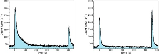
Lightcurves in the 0.5–10.0 keV range of bursts of 15, 16 (left-hand panel) and 21 and 22 (right-hand panel). The time resolution in these light curves is 1 s and pre-burst count rates are not subtracted.
3.1 Time resolved spectroscopy
3.1.1 Application of different background approaches
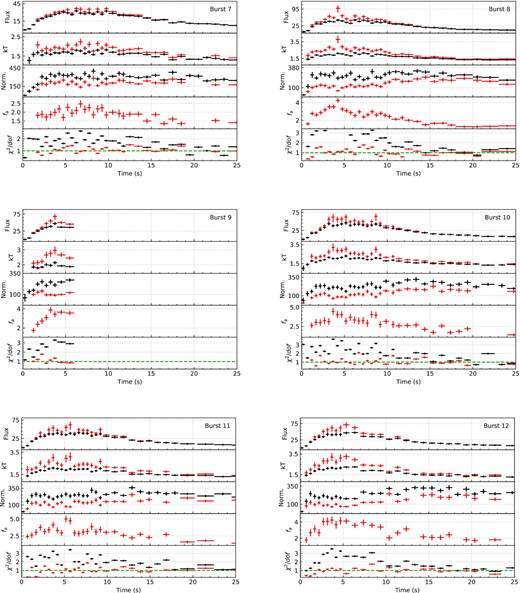
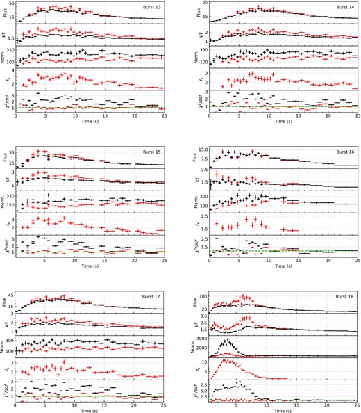
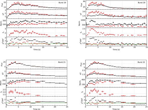
Combining the unique soft X-ray sensitivity with the relatively large number of bursts observed from the source gives us a chance to test different approaches used to fit time resolved X-ray spectra of bursts. The resulting spectral evolution for each burst are summarized in Figs B1–B4 in Appendix B. These figures show time evolution of flux, blackbody temperature and the blackbody normalization as inferred from the fits as well as the χ2 values. For a better comparison, in each figure we show the results for both fixed background approach and the fa method, with best fit fa values shown in a separate panel. As is evident from figures in Appendix B, especially around the peaks, the fixed background approximation does not provide a statistically acceptable fit. To test the energy dependency of the fits, we also applied the fixed background model in the 3.0–10.0 keV range. Such an approach resulted in better fits indicating that the poorer fits in the 0.5–10.0 keV range results mostly due to excess emission in the soft X-rays. The resulting spectral evolution using only the data in the 3.0–10.0 keV range is shown for bursts 18 and 20 in Fig. 4 as an example.
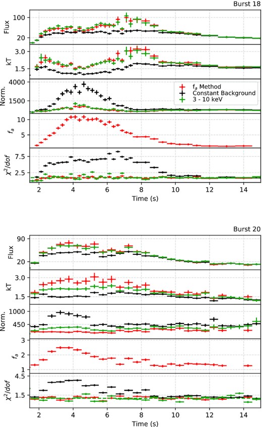
Time evolutions of spectral parameters are shown for Burst 18 and 20. We show, from top to bottom: The bolometric X-ray flux, the blackbody temperature, the blackbody normalization (in units of R|$^2_{\rm km}/\rm {D}_{10 {\rm kpc}}^{2}$|), fa and finally, the fit statistic. The red symbols show the results of the fa method, black and green symbols show the results for constant background approach but in the 0.5–10.0 keV or 3–10.0 keV energy ranges, respectively.
In Fig. 5, we show the resulting distributions of χ2 values for X-ray spectra where the bolometric burst flux is above 10−9 erg s−1 cm−2. Such a flux limit is selected because at this level the burst flux becomes comparable to the pre-burst flux of the source (see Table 2). The χ2 distributions show that fixed background approach to the time resolved X-ray spectra in the 0.5–10.0 keV range do not provide statistically acceptable fits for a large number of X-ray spectra. In total, we have 1041 X-ray spectra down to the specified flux limit and in 68 per cent of this sample (707 spectra) adding an fa component caused a statistically significant improvement in the fits. Fig. 6 shows the histogram of the best fit fa values, where the bolometric flux and fa are greater than 10−9 erg s−1 cm−2 and 1.0, respectively. Note that in Fig. 6, fa values for burst 18 are shown in a different colour to emphasize the fact that the largest fa values are obtained when the burst shows evidence for PRE.
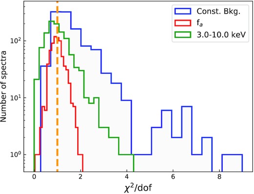
Histograms of all the χ2/dof values using constant background or the fa method as well as the resulting statistics values when we only fit to the data in the 3–10 keV range. Only the results where the burst flux is above 10−9 erg s−1 cm−2 are included here. The statistical improvement, in cases where an adding an fa parameter is the preferred model can be seen. Orange vertical line shows the case where χ2/dof = 1.
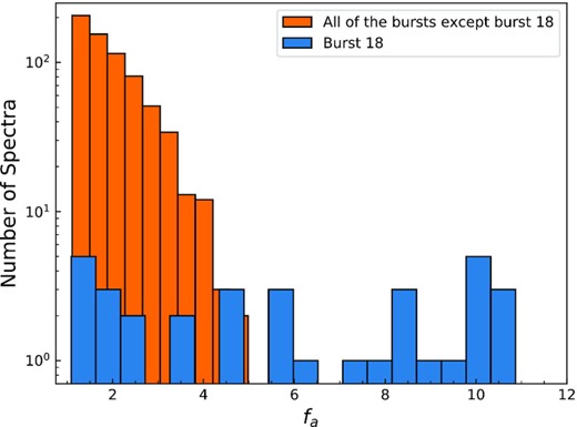
Distribution of fa values including all of the X-ray spectra where the flux is above 10−9 erg s−1 cm−2 except the fa values obtained from burst 18, is shown in orange. We also show the fa values inferred from only burst 18 with blue, where a PRE is observed.
In Fig. 7, we show the best-fitting spectral parameters inferred using either the classical fixed background method or the fa method. It can be seen that because the 0.5–10 keV X-ray spectra extracted from bursts are broader than a pure blackbody, using the fixed background approach results in blackbody temperatures that are significantly lower and normalization values that are significantly larger than the parameters as inferred using the fa method. The colour coding in Fig. 7 shows that the difference in temperature and normalization grows with the magnitude of fa. In the same figure, we also show with grey colour the results inferred from fitting only the 3–10 keV band. The spectral parameters obtained in this higher energy band do not show the variations in temperature and normalization found in the full band, implying that these approaches agree with each other much better. These results suggest that the best-fitting spectral parameters obtained in the RXTE/PCA era were mostly free of the soft X-ray excess (e.g. Galloway et al. 2008; Güver et al. 2012a; Güver, Özel & Psaltis 2012b; Özel et al. 2016), however a detailed analysis is beyond the scope of this paper and may not be possible given the decreasing effective area of NICER towards higher energies. The fact that NICER has a larger effective area in the soft X-ray band likely further alters the best-fitting spectral parameters. The same trend can also be seen in Fig. 8 where we show the histograms of blackbody temperature and normalization values for the three different fitting approaches.
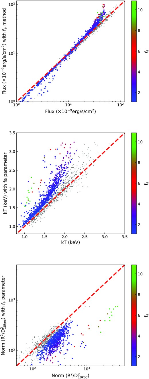
From top to bottom comparison of flux, blackbody temperature and blackbody normalization values obtained with or without applying the fa method (from top to bottom) as a function of fa value. In each panel we also include the results from fits to only the 3–10 keV range with grey dots, which show a much better agreement with the results obtained from fa method.
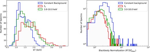
Histogram of blackbody temperature (left panel) and normalization (right panel) values with or without the fa method. Each curve represents the constant background, the fa, and energy range of 3.0–10.0 keV with the colours blue, red, and green, respectively. We include all of the X-ray spectra where the bolometric flux and fa are greater than 10−9 erg s−1 cm−2 and 1.0, respectively.
Such significant variations in the spectral parameters can even affect the identification of a burst as a PRE event. Using the fixed background approach, we find two bursts showing evidence for a PRE. In burst 18, the normalization of the blackbody reaches to 36 km, which then decreases down to about 9.7 km, assuming a source distance of 6.0 kpc. In burst 20, the blackbody normalization reaches up to 18 km before normalizing to about 12 km after touchdown. By all definitions (Galloway et al. 2008; Güver et al. 2012b) these values show evidence for a PRE. However in both cases during these episodes the fixed background approach results in significantly worse fits to the data if the whole NICERband (0.5–10.0 keV) is used. If the fa method is employed, the models provide much better fits to the data but this also strongly affects the inferred values in the blackbody normalization and temperature. The evidence for a PRE in burst 20 disappears completely, while for burst 18 a spectral evolution as expected from a PRE event can still be seen. The variation in the spectral parameters can be seen in Fig. 4. We note that when only the 3–10 keV band is used the spectral evolution closely matches the evolution inferred from the fa method.
We also present in Table 3 the best-fitting parameters obtained for each burst at the peak flux moment using the two methods as well as the fluences of each burst. We calculated the fluences by integrating all the flux values found via the fa method, starting from the beginning of a burst till the flux is less than 10 per cent of the peak following Güver et al. (2021).
Spectral parameters obtained at the peak flux moment for each burst with or without the application of the fa method are shown. Fluence of each burst is also presented. The fluences are calculated using the results of the fa method.
| Burst no. | fa at peak | Peak fluxa | kT at peak (keV) | BB Norm at peak | Fluenceb | |||
|---|---|---|---|---|---|---|---|---|
| with fa | without fa | with fa | without fa | with fa | without fa | with fa | ||
| 1 | 3.2 ± 0.4 | 1.7 ± 0.5 | 1.7 ± 0.1 | 2.8 ± 0.5 | 1.6 ± 0.1 | 30 ± 13 | 229 ± 28 | 11.2 ± 0.5 |
| 2 | 3.0 ± 0.4 | 4.2 ± 0.5 | 3.6 ± 0.3 | 2.3 ± 0.2 | 1.9 ± 0.1 | 137 ± 26 | 257 ± 27 | 24.2 ± 0.7 |
| 3 | 2.1 ± 0.1 | 6.0 ± 0.7 | 4.4 ± 0.4 | 2.6 ± 0.2 | 1.9 ± 0.1 | 132 ± 21 | 307 ± 33 | 49 ± 0.9 |
| 4 | 2.1 ± 0.2 | 4.7 ± 0.5 | 3.9 ± 0.3 | 2.2 ± 0.1 | 1.8 ± 0.1 | 189 ± 28 | 345 ± 35 | 37 ± 0.7 |
| 5 | 2.0 ± 0.2 | 4.4 ± 0.4 | 3.8 ± 0.3 | 2.1 ± 0.1 | 1.8 ± 0.1 | 195 ± 28 | 326 ± 33 | 37 ± 0.7 |
| 6 | 2.3 ± 0.2 | 4.4 ± 0.5 | 3.7 ± 0.3 | 2.3 ± 0.2 | 2.0 ± 0.1 | 151 ± 24 | 264 ± 29 | 41.7 ± 0.9 |
| 7 | 2.1 ± 0.2 | 3.6 ± 0.3 | 3.3 ± 0.3 | 2.1 ± 0.1 | 1.8 ± 0.1 | 184 ± 27 | 288 ± 30 | 42.0 ± 0.8 |
| 8 | 4.3 ± 0.3 | 9.8 ± 1.5 | 5.0 ± 0.5 | 3.8 ± 0.4 | 2.2 ± 0.1 | 58 ± 13 | 212 ± 25 | 60.6 ± 1.6 |
| 9 | 3.5 ± 0.3 | 6.8 ± 0.9 | 4.7 ± 0.5 | 3.0 ± 0.3 | 2.1 ± 0.1 | 91 ± 17 | 212 ± 25 | 15.9 ± 0.9 |
| 10 | 4.0 ± 0.4 | 6.4 ± 1.0 | 4.6 ± 0.5 | 3.0 ± 0.3 | 2.3 ± 0.2 | 83 ± 19 | 160 ± 22 | 41.5 ± 1.2 |
| 11 | 4.7 ± 0.5 | 6.2 ± 1.1 | 4.1 ± 0.4 | 3.1 ± 0.4 | 2.0 ± 0.1 | 72 ± 19 | 255 ± 33 | 37.3 ± 1.1 |
| 12 | 4.1 ± 0.3 | 7.1 ± 0.9 | 4.7 ± 0.4 | 3.3 ± 0.3 | 2.3 ± 0.1 | 69 ± 12 | 178 ± 16 | 32.0 ± 1.3 |
| 13 | 3.0 ± 0.3 | 4.6 ± 0.6 | 3.6 ± 0.3 | 2.6 ± 0.3 | 1.9 ± 0.1 | 97 ± 21 | 248 ± 28 | 48.9 ± 1.1 |
| 14 | 2.4 ± 0.2 | 4.4 ± 0.5 | 3.7 ± 0.3 | 2.4 ± 0.1 | 2.0 ± 0.1 | 119 ± 20 | 214 ± 24 | 41.1 ± 0.9 |
| 15 | 3.1 ± 0.3 | 5.9 ± 0.8 | 4.2 ± 0.3 | 3.0 ± 0.3 | 2.1 ± 0.1 | 80 ± 16 | 191 ± 16 | 41.6 ± 1.3 |
| 16 | 1.8 ± 0.2 | 1.4 ± 0.2 | 1.3 ± 0.1 | 1.8 ± 0.2 | 1.7 ± 0.1 | 115 ± 29 | 165 ± 26 | 10.9 ± 0.3 |
| 17 | 3.1 ± 0.3 | 4.3 ± 0.5 | 3.4 ± 0.3 | 2.4 ± 0.2 | 2.0 ± 0.1 | 121 ± 22 | 215 ± 23 | 40.7 ± 1.0 |
| 18 | 5.8 ± 0.4 | 10.0 ± 1.6 | 4.9 ± 0.4 | 3.1 ± 0.3 | 1.9 ± 0.1 | 121 ± 27 | 323 ± 37 | 47.7 ± 1.4 |
| 19 | 2.3 ± 0.2 | 5.5 ± 0.7 | 4.2 ± 0.4 | 2.7 ± 0.2 | 2.1 ± 0.1 | 107 ± 18 | 208 ± 24 | 45.7 ± 1.0 |
| 20 | 2.5 ± 0.1 | 7.7 ± 1.0 | 5.1 ± 0.4 | 2.9 ± 0.3 | 1.8 ± 0.1 | 115 ± 25 | 466 ± 47 | 53.3 ± 1.4 |
| 21 | 2.4 ± 0.3 | 2.6 ± 0.3 | 2.3 ± 0.2 | 1.9 ± 0.2 | 1.7 ± 0.1 | 170 ± 30 | 261 ± 26 | 10.7 ± 0.3 |
| 22 | 3.5 ± 0.3 | 3.7 ± 0.4 | 3.0 ± 0.2 | 2.2 ± 0.2 | 1.7 ± 0.1 | 138 ± 23 | 381 ± 36 | 18.6 ± 0.5 |
Unabsorbed bolometric flux in units of × 10−8 erg s−1 cm−2.
Fluence in units of × 10−8 erg cm−2.
From the Fig. A3, it can be seen that burst 20 shows evidence for a secondary peak ≈6 s after the start of the burst. From the light curve alone the secondary peak resembles the secondary peaks previously observed from 4U 1608 − 52 by NICER (Jaisawal et al. 2019; Güver et al. 2021). Time resolved spectroscopy of the burst does not show a significant spectral evolution when the routine time resolution is used, which in this case is 0.5 s (see Fig. B4). To test whether somewhat more detail can be detected we also generated X-ray spectra with 0.25 s time resolution. The results of the fa method fits to these spectra are shown in Fig. 9. While a jump in the blackbody temperature near the secondary peak can be seen, the large statistical uncertainties prevent any conclusion.
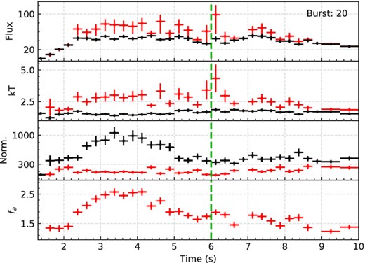
Spectral evolution observed in Burst 20. The location of the secondary peak is marked with a green dashed line. Time resolution used here is 0.25 s that shows more detail around the secondary peak observed in the light curve.
A histogram of all the fa values obtained are shown in Fig. 6. It can be seen that in a great majority of the cases the best fit fa values are within 1–3. Only in burst 18, fa values as high as 11 are observed. These findings are mostly in line with the findings of Worpel et al. (2015), where it is shown that fa values are smaller in bursts showing no evidence for a PRE. Fragile et al. (2018, 2020) performed simulations of accretion discs subjected to burst emission surrounding a neutron star for thick and thin accretion disc assumptions, respectively. In both cases, they predict a significant increase in the mass accretion rate on to the neutron star, which is mainly driven by the Poynting-Robertson drag (Robertson 1937; Blumenthal 1974; Walker & Meszaros 1989; Walker 1992). The predicted increase in the accretion rate for an Eddington limited burst is as large as an order of magnitude in the case of a thin accretion disc. As a multiplicative factor to the pre-burst spectral model fa values greater than one, are typically attributed to increased accretion rates. Our results show that bursts from Aql X-1 also show similar episodes of increased mass accretion rates. The maximum fa values reached in bursts indicate increased episodes of mass accretion rate by a factor of 2 to 11.
Fig. 10 shows the relation between the maximum fa value reached during the burst and the fa value at the peak flux moment. We observe that the maximum fa value reached during a burst is often at the peak flux moment. The Spearman’s rank correlation coefficient between the fa value at the peak flux moment of a burst and the maximum fa reached is calculated as 0.96 with a p-value of 4 × 10⁻¹², excluding burst 18. In the case of burst 18, there is a remarkable difference in between the fa value at the peak flux moment and the maximum fa value reached, which roughly corresponds to the maximum of the observed blackbody normalization i.e., the maximum photospheric radius expansion moment. Although the fa value at the peak flux and the maximum fa reached during a burst are often correlated there are also differences. The time difference between the peak flux moment and the moment fa reached its maximum may provide information on the accretion flow’s response to the burst, if fa probes the mass accretion rate on to the neutron star as suggested. Simulations performed by Fragile et al. (2020) suggest that the increase in the mass accretion rate on to the neutron star precedes the peak flux moment. In Fig. 11, we show the time difference between the moment fa value reached its maximum and the moment a burst reached its peak flux. Within the 22 bursts investigated here, the time difference is within the ±0.5 s in 12 bursts, showing no significant time difference. In seven bursts, the fa reaches its maximum value before the burst reaches its peak flux with an average time difference of 2.5 s. These differences are in line with predictions from simulations (Fragile et al. 2020), where the mass accretion rate on to the neutron star shows increase before the burst reaches the peak. Simulations also provide insight into the time difference between when Compton cooling of the plasma in the disc is taken into account and not. In the absence of Compton cooling the time difference between the peak flux of the burst and the maximum of the increase in the mass accretion rate is expected to be smaller. Since the efficiency of Compton cooling depends on the location of the corona (Degenaar et al. 2018), variations in the efficiency of Compton cooling may explain the two groups we observe here. Although not very strongly, we also found that the peak flux of a burst is correlated with the fa value obtained at that moment. The correlation coefficient between the peak flux of a burst and the fa at peak is 0.66. It is obvious that the brighter the burst is, the larger the observed fa, meaning the deviation from a pure blackbody model is stronger. This relation is shown in Fig. 12.
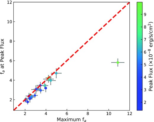
Relation between the maximum fa value reached during a burst and the fa at the peak flux moment. The colour coding shows the peak flux reached in each burst.
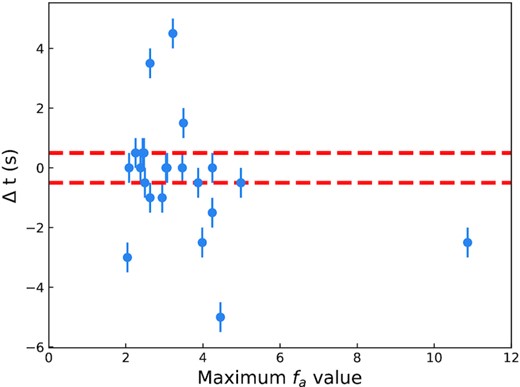
The time difference between the moment the accretion rate reached maximum (fa value reached its maximum) and the peak flux moment of a burst as a function of the maximum fa value. Horizontal red dashed lines show the ±0.5 s time difference region. Since the integration time we used for the spectral analysis is 0.5 s it would be impossible to infer smaller time differences.
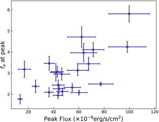
Correlation between the maximum fa value and the peak flux in a burst.
3.1.2 Application of reflection model
Results of the reflection model fits show once again a significant improvement compared to blackbody fits with fixed background. We find that in each case the ionization parameter of the reflection model reaches the upper limit of the tabulated values, indicating that the accretion disc is strongly ionized by the burst emission. The resulting distribution of the χ2 values of the three different methods for the peaks of the bursts are shown in Fig. 13. It can be seen that while the reflection model improves the goodness of the fit, fa method still provides a statistically better result with one less free parameter. The fact that the ionization parameter of the reflection model is pegged at the largest value of the tabulated model means that we are basically fitting the bremsstrahlung continuum to model the soft excess, with only free parameter being the normalization or the flux of the reflection component, since the density in the disc is fixed. However, it is expected that the reflection fraction should be 20–30 per cent of the burst emission itself (Keek et al. 2018a), which depends on the inclination angle of the system as well as the inner disc radius. A comparison of the inferred burst and reflection model fluxes at the peak moments of each burst is shown in the left-hand panel of Fig. 14. From our fits, we can infer that while this generally holds true for all of the bursts, in two bursts where simple blackbody approximation results show evidence for a PRE (burst 18 and 20), the inferred flux of the reflection model exceeds the burst emission itself. This result shows that the application of the reflection model at the peak of the bursts with PRE is actually not enough just by itself and a further soft component is required.
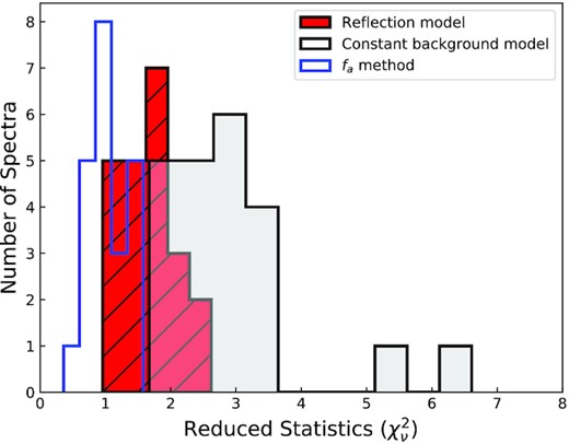
Histogram comparing of the reduced χ2 values obtained at the peak flux moment of each burst using simple blackbody, fa, and reflection model methods.
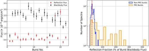
Left panel: 0.5–10.0 keV fluxes of the burst blackbody emission and the reflection component at the peak flux moment of each burst. Right panel: Flux of the reflection component in units of burst blackbody emission fraction for all the burst. Blue histogram shows the reflection fraction for non-PRE bursts, while the orange histogram shows the fraction for the bursts that show evidence for a PRE. Red vertical dashed line shows the peak of the distribution for the non-PRE bursts which is 20 per cent.
As a second approach we also fitted all of the X-ray spectra where fa was statistically required in all of the bursts. The ionization parameter values throughout the bursts still hit the upper limit of the tabulated models. However, the flux ratio of the reflection models compared to the burst emission shows a very similar distribution to what we obtained from fitting only the peaks of the bursts. A histogram of the flux ratios of the reflection models and the burst blackbody emission is shown in the right-hand panel of Fig. 14. We see that while in a great majority of the spectra in non-PRE bursts the flux of the reflection model is around 20 per cent of the burst emission itself, in bursts where there is some evidence for a PRE and especially at around the peak fluxes the fraction of the flux of the reflection models exceeds the incident flux from the burst blackbody indicating that the results are not physical. We can therefore conclude that especially at the peaks of these bursts the reflection model only helps to somehow improve the fits but is not enough by itself to result in a physically reasonable fit. We note that for burst 18 we also tried to fit the spectra with both the reflection model as well as the fa parameter. However, the existing spectral data does not allow us to constrain the parameters of the reflection model and the fa at the same time.
4 DISCUSSION AND CONCLUSIONS
Observations of low-mass X-ray binaries showing X-ray bursts, like Aql X-1, 4U 1820-30, SAX J1808.4-3658, Swift J1858.6-0814, MAXI J1807 + 132, XTE J1739-285, and 4U 1608-52 (Keek et al. 2018a,b; Bult et al. 2019, 2021a; Buisson et al. 2020; Albayati et al. 2021; Güver et al. 2021) already demonstrated the power of NICER in probing the effects of X-ray bursts on their accretion environments. Here, we follow-up on these studies by investigating an ensemble of 22 X-ray bursts observed from Aql X-1 across accretion states by NICER to better understand the spectral evolution especially in the soft X-ray band. First of all, the existing NICER data set from Aql X-1 already shows some interesting bursts. As noted, there are two bursts (18 and 20) showing evidence for a PRE. However, the use of the fa method affects the inferred spectral parameters in a way that minimizes the evidence for a PRE.
In burst 20 the light curve shows a significant secondary peak, roughly about 6 s after the burst start. However, the spectral evolution does not show a similarly significant change in the spectral parameters at the expected time. Within our sample this is the only burst which happens at a relatively high mass accretion rate as inferred from the flux of the pre-burst emission. Assuming the Eddington limit of the source as FEdd = 10.44 × 10⁻⁸ erg s−1 cm−2 (Güver et al. 2012b), we can infer that the source was emitting roughly at 10 per cent Eddington limit level just before this burst. This level is in agreement with the bursts observed from 4U 1608 − 52, showing secondary peaks when the system was emitting at about 15 per cent of the Eddington limit (Güver et al. 2021).
Bursts 15, 16 and 21 and 22 are also worth noting given that they can be classified as short recurrence bursts with separations of only 496 s and 451 s, respectively. These recurrence times are some of the shortest in the MINBAR catalogue both for Aql X-1 and for all the bursters in general (Galloway et al. 2020). The minimum reported value is 233 s for 4U 1705–44 in the MINBAR catalogue (Keek et al. 2010; Galloway et al. 2020). Most recently, bursts 21 and 22 have been reported to happen 9.44 days after a superburst (Li, Pan & Falanga 2021). We note that burst 20 reported here happened only three days before the reported superburst. It is also interesting to further emphasize the fact that in the case of bursts 21 and 22, where the separation of the two events is only 451 s, the second burst is brighter than the first one. To the best of our knowledge, such a short recurrence event has not been reported before in the existing catalogues (Keek et al. 2010; Galloway et al. 2020). The peak count rate of burst 21 is only 75 per cent of burst 22, while the peak flux of the blackbody component when the fa method is used is only 70 per cent of burst 22. The difference is even more significant when the fluences of each burst is compared, the fluence of burst 21 is only 54 per cent of burst 22. Boirin et al. (2007) reports a triple burst from EXO 0748-676, where the third burst is brighter than the second one but still somewhat dimmer than the first burst. However, prior to burst 21 there is data for only 600 s, which is not enough to test whether this was another triple burst event or not.
We also searched for burst oscillations in three different energy bands in all of observed X-ray bursts from Aql X-1. We found no significant burst oscillation within the NICERsample. Our upper limits on the fractional rms amplitudes are typically around 0.05, which is similar to the limits presented in other studies (Ootes et al. 2017; Galloway et al. 2020) and smaller than the amplitudes of the previously reported oscillations. Within the MINBAR catalogue roughly only 10 per cent (8 bursts) of all the bursts from Aql X-1 showed significant burst oscillations and 6 of those were bursts showing PRE. In our case, we only have two bursts showing evidence for a PRE. In burst, 18 our limits are as small as 0.02. Based on the amplitudes of previously reported oscillations, we can rule out the existence of burst oscillations in that burst.
We performed time resolved spectroscopy of the bursts within the NICERband to better understand the soft X-ray emission observed during the bursts from these systems. Shortly after NICER started observations of X-ray bursters, evidence for a strong soft excess in the soft X-ray band of the time resolved spectra of bursts have been reported (Keek et al. 2018a,b; Bult et al. 2021b). Hints about such an excess has already been known and could be studied in some cases (Ballantyne & Strohmayer 2004; Worpel et al. 2013, 2015). We here provide a more systematic study of these deviations using all of the X-ray bursts observed so far from Aql X-1. We see that the application of the fa model statistically improves the fits, indicating that the burst strongly affects the surrounding accretion disc. However, the fa model by itself does not provide a detailed physical insight of the observed increase in the pre-burst emission. It is generally thought that the observed increase in the pre-burst emission is indicative of increased mass accretion rate (Worpel et al. 2013, 2015) to the neutron star. In accordance with such expectations, recent simulations by Fragile et al. (2020) predict a detectable yet temporary increase in the accretion rate on to the neutron star, mostly due to Poynting-Robertson drag during a burst. The maximum fa values inferred here are in agreement with theoretical predictions. Simulations also predict the mass accretion rate to increase a few seconds before the burst reaches its peak. We find that in about 7 bursts we can observe a similar time difference. It is expected that the disc-burst interaction should be a function of burst luminosity and therefore the amount of soft excess should depend on, for example, the peak flux of a burst. Our results indicate that, although with some scatter, indeed there is such a relation (see Fig. 12). The deviation from a pure blackbody becomes strongest at the peak flux moment of each burst and the actual amount of deviation or soft excess depends on the peak flux of a burst. The fa model nicely illustrates that point. We note that, although X-ray bursts show short time scale variations and therefore integration times used to extract spectra may have an effect of averaging different temperatures, the deviation observed here was also observed from 4U 1820 − 30 (Keek et al. 2018b), where the exposure times used for individual spectra were as short as 0.03 s.
There may be several reasons for the burst emission to show deviations from a pure blackbody. First of all, atmospheric effects are expected to play a significant role (for a review see e.g. Özel 2013). All of the bursting neutron star atmosphere models (see e.g. Madej, Joss & Różańska 2004; Majczyna et al. 2005; Suleimanov, Poutanen & Werner 2011) predict significantly broadened X-ray spectra compared to a pure blackbody. Furthermore, given the fact that these systems often contain rapidly rotating neutron stars, relativistic affects also have the potential to broaden the observed X-ray spectra (Bauböck et al. 2015). However, in both cases the predicted deviations from a blackbody emission are practically time independent, whereas the deviations we report here show significant variations during an X-ray burst.
One likely interpretation of the excess emission observed during X-ray bursts may be related to the reflection of the burst emission by the accretion disc. We used a tabulated reflection model assuming solar abundances to see if the reflection models can improve the fits to the X-ray spectra and provide an understanding of the reflection processes. Our results indicate that indeed reflection models do improve the fits and can account for the soft excess but not as well as the fa model. The best-fitting ionization parameters of the used models were very high, allowing us to only put lower limits on that parameter. This indicates that the accretion disc is highly ionized. Still, the inferred 0.5–10.0 keV flux ratios of the best-fitting blackbody models and the reflection models are generally in line with what is expected (at around 20% level), which shows that reflection may be a common feature in the X-ray spectra of bursts, and can be detected. In two bursts where we see some evidence of a PRE, the reflection model and blackbody model fractions reverses with reflection fractions much larger than the intrinsic burst flux. This indicates that during these bursts some other processes may also have a significant effect on the soft X-ray excess and therefore reflection model just by itself is not enough.
Finally, we compared the best-fitting spectral parameters for the peaks of the bursts with the parameters obtained from the bursts in the MINBAR catalogue (Galloway et al. 2020). We show in Fig. 15 the bolometric flux and blackbody temperature values inferred at the peaks of the bursts in the MINBAR catalog observed mostly with RXTE/PCA together with the best-fitting values we find via different methods here. When combined with the results shown in Figs 7 and 8, it obvious that the use of different methods result in a significant variation in the inferred blackbody temperature and flux as compared to the archival measurements. It is likely that these results advocate the need for broad-band studies that can readily be performed by simultaneous observations of NICER and ASTROSAT (Yadav et al. 2017) or with future large effective area detectors like STROBE-X (Ray et al. 2019) or eXTP (Zhang et al. 2019) in order to be able to both determine the spectral parameters of the bursts as well as their effects on the surrounding environments precisely. Even now, NICER observations of X-ray bursts from sources with low hydrogen column density will provide a unique view on what impact do thermonuclear X-ray bursts have on their surroundings, thanks to its soft X-ray sensitivity and expanding archive of burst observations.
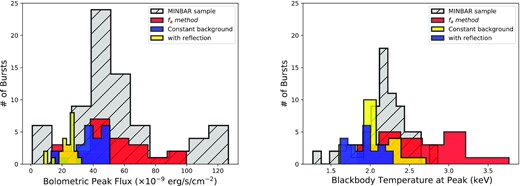
Comparison of spectral parameters obtained at the peak moments of each burst with archival bursts from MINBAR catalogue (Galloway et al. 2020). The histogram of spectral parameters for the archival bursts are shown with grey, while with blue the distribution of the spectral parameters as found from classical blackbody fits, with red the spectral parameters found from the fa method, and with yellow the spectral parameters as inferred taking into account the reflection is shown. Note that from the MINBAR catalog we only used results of the bursts observed by RXTE/PCA.
ACKNOWLEDGEMENTS
We gratefully thank the anonymous referee for constructive comments and recommendations. We thank Rümeysa Aslıhan Ertürk for her contribution on writing some of the scripts used in this paper. TG has been supported in part by the Scientific and Technological Research Council (TÜBİTAK) 119F082 and the Turkish Republic, Presidency of Strategy and Budget project, 2016K121370. DA thanks the Royal Society for their support. This work was supported by NASA through the NICER mission and the Astrophysics Explorers Program. This research has made use of the data and software provided by the High Energy Astrophysics Science Archive Research Center (HEASARC), which is a service of the Astrophysics Science Division at NASA/GSFC and the High Energy Astrophysics Division of the Smithsonian Astrophysical Observatory.
DATA AVAILABILITY
All the data used in this publication is publicly available through NASA/HEASARC archives.
Footnotes
REFERENCES
APPENDIX A: LIGHT CURVES OF BURSTS
Light curves of each burst as observed in the 0.5–10.0 keV range are given together with the burst start, peak, and decaying e-folding times.

Background subtracted of 0.5−10.0 keV light curves of detected thermonuclear X-ray bursts with NICER.
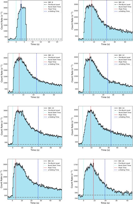
Same as Fig. A1. Note that the observation stopped just after the peak of burst 9.

Same as Fig. A1.
APPENDIX B: TIME EVOLUTION OF SPECTRAL PARAMETERS FOR EACH BURST
Figures of time resolved spectral evolution for all the bursts are shown here.
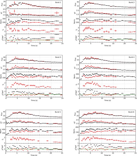
Time evolution of spectral parameters are shown. Red symbols show the results of fa method and black symbols show the results for constant background case. We show, from top to bottom: the 0.5–10 keV X-ray flux, the temperature, the blackbody normalization, fa and finally, the fit statistic. In all panels fluxes are bolometric and in units of × 10−9 erg s−1 cm−2. The temperature and blackbody normalization are in units of keV and |$R^2_{km}/D^2_{10\rm {kpc}}$|, respectively.
Same as Fig. B1.
Same as Fig. B2.
Same as Fig. B3.
