


ABSTRACT
It is clear that within the class of ultra-diffuse galaxies (UDGs), there is an extreme range in the richness of their associated globular cluster (GC) systems. Here, we report the structural properties of five UDGs in the Perseus cluster based on deep Subaru/Hyper Suprime-Cam imaging. Three appear GC-poor and two appear GC-rich. One of our sample, PUDG_R24, appears to be undergoing quenching and is expected to fade into the UDG regime within the next ∼0.5 Gyr. We target this sample with Keck Cosmic Web Imager (KCWI) spectroscopy to investigate differences in their dark matter haloes, as expected from their differing GC content. Our spectroscopy measures both recessional velocities, confirming Perseus cluster membership, and stellar velocity dispersions, to measure dynamical masses within their half-light radius. We supplement our data with that from the literature to examine trends in galaxy parameters with GC system richness. We do not find the correlation between GC numbers and UDG phase space positioning expected if GC-rich UDGs environmentally quench at high redshift. We do find GC-rich UDGs to have higher velocity dispersions than GC-poor UDGs on average, resulting in greater dynamical mass within the half-light radius. This agrees with the first order expectation that GC-rich UDGs have higher halo masses than GC-poor UDGs.
1 INTRODUCTION
While the existence of large, low surface brightness galaxies has been known for many decades (e.g. Disney 1976; Sandage & Binggeli 1984; Bothun et al. 1987; Impey, Bothun & Malin 1988; Impey & Bothun 1997), the work of van Dokkum et al. (2015) has reignited interest in their study. The latter study identified 47 low surface brightness within the Coma cluster and established the working definition of ‘ultra-diffuse galaxy’ (UDG) based on two criteria: half-light radius, Re > 1.5 kpc, and surface brightness, μ0,g > 24 mag arcsec−2 (van Dokkum et al. 2015).
Many UDGs have been shown to host extensive globular cluster (GC) systems (e.g. Beasley & Trujillo 2016; Beasley et al. 2016; van Dokkum et al. 2017, 2018b; Amorisco et al. 2018; Lim et al. 2018, 2020; Toloba et al. 2018; Forbes et al. 2019; Prole et al. 2019; Román et al. 2019; Somalwar et al. 2020; Montes et al. 2020, 2021; Müller et al. 2021; Shen, van Dokkum & Danieli 2021). It has been demonstrated that dense environments can impact a galaxy’s GC system, increasing the GC system richness relative to the stellar mass (i.e. the GC specific frequency; Peng et al. 2008; Liu et al. 2016; Lim et al. 2018). Early indications are that this is also true for UDGs, particularly in the Coma cluster (Lim et al. 2018; Forbes et al. 2020; Somalwar et al. 2020). Three possible explanations for this effect have been proposed in the literature: 1) increased GC production due to the earlier and faster formation times of cluster galaxies, 2) decreased GC destruction due to earlier quenching times, and 3) decreased field star formation due to earlier quenching times (see e.g. Peng et al. 2008; Carlsten et al. 2021).
Interestingly, these explanations align with some proposals for forming the large sizes and/or low surface brightnesses of UDGs. Rapid star formation timescales will introduce a sharp impulse of energy into the system, which has been studied as a possible avenue for creating UDG’s large sizes (e.g. Di Cintio et al. 2017; Chan et al. 2018; Jiang et al. 2019; Martin et al. 2019). Early infall times will quench star formation resulting in a passively evolving stellar population that will slowly decrease in surface brightness (e.g, Yozin & Bekki 2015; Román & Trujillo 2017; Chan et al. 2018; Jiang et al. 2019; Sales et al. 2020; Tremmel et al. 2020). Additionally, UDGs that fall in earlier will spend more time being subject to the cluster’s tidal forces, which can play an important role in heating and expanding UDG stellar populations, giving rise to their large sizes (Yozin & Bekki 2015; Jiang et al. 2019; Martin et al. 2019; Carleton et al. 2019, 2021; Sales et al. 2020). Other mechanisms (e.g. high halo spin; Amorisco & Loeb 2016; Rong et al. 2017; Mancera Piña et al. 2020) and combinations of mechanisms (e.g. stellar feedback and quenching, Chan et al. 2018 or stellar feedback and tides, Jiang et al. 2019) have also been considered.
Up until now, simulations of UDG formation have primarily focused on the formation of their stellar body (see e.g. Yozin & Bekki 2015; Di Cintio et al. 2017; Chan et al. 2018; Carleton et al. 2019; Jiang et al. 2019; Liao et al. 2019; Martin et al. 2019; Sales et al. 2020; Tremmel et al. 2020; Wright et al. 2021) but very few have focused on modelling their associated GC systems. Large cosmological simulations of galaxy formation do not (yet) have the resolution to properly resolve GC formation. Probing galaxy GC formation requires either the implementation of specialized simulations for single galaxies (e.g. Dutta Chowdhury, van den Bosch & van Dokkum 2020) or additional sub-grid/semi-analytic modelling within the simulation (e.g. Carleton et al. 2021; Doppel et al. 2021). To date, only one work has applied such semi-analytic models to a cosmological simulation to investigate GC formation in UDGs. Carleton et al. (2021) used a semi-analytic model for GC formation along with the IllustrisTNG simulations to find that UDGs with large GC populations likely formed through a combination of fast, high-redshift star formation and tidal heating in a cluster environment.
The effects of external tidal fields acting on a UDG is highly dependent on the structure of its dark matter halo (e.g. cusp versus core and total mass). GCs are a known indicator of total dark matter halo mass for normal galaxies (Spitler & Forbes 2009; Harris, Harris & Alessi 2013; Harris, Blakeslee & Harris 2017; Burkert & Forbes 2020). Currently this relation has only one independent confirmation for UDGs coming from a resolved mass profile for the UDG Dragonfly 44 (van Dokkum et al. 2019b; Forbes et al. 2021). Using the Burkert & Forbes (2020) relation, Forbes et al. (2020) studied the GC systems of UDGs in the Coma cluster and suggested the existence of two types of UDG dark matter halo. One type is GC-poor with dwarf-like dark matter haloes (MHalo ≈ 1010 M⊙) and the other is GC-rich with massive, 1011 − 1012 M⊙ dark matter haloes. Many authors propose these GC-rich UDGs may be examples of ‘failed galaxies’ that were rapidly quenched after a period of early, rapid star formation (van Dokkum et al. 2017; Forbes et al. 2020; Villaume et al. 2021). The population of GC-poor UDGs is expected to be more mixed, resembling ‘puffy dwarf’ galaxies - normal dwarfs that have been ‘puffed up’ through a variety of processes to larger sizes and low surface brightnesses. We note the existence of tidal UDGs (e.g. Ogiya 2018; Collins et al. 2020; Iodice et al. 2021; Román et al. 2021) and other low dark matter UDGs which will not fit into these two types but this is beyond the scope of this work.
Mass measurements coming from stellar, and GC velocity dispersions, for many GC-rich UDGs confirm their dark matter dominated nature (Beasley et al. 2016; van Dokkum et al. 2016, 2017, 2019b; Toloba et al. 2018; Martín-Navarro et al. 2019; Gannon et al. 2020, 2021; Forbes et al. 2021). When used in comparison to a total halo mass estimate coming from GC numbers they can be used to infer basic halo properties (e.g. cusp versus core) (Toloba et al. 2018; Gannon et al. 2020, 2021; Forbes et al. 2021).
Also of importance in studying external environmental effects on UDGs, such as early quenching, are their position – velocity locations within their environment (Alabi et al. 2018). To first order, galaxies populate distinct regions in phase space which are dependent on their infall time (Rhee et al. 2017). UDGs that have spent longer in the higher density environment will have quenched earlier and will have been subjected to its tidal field for a longer period (see section 5.2 of Martin et al. 2019 for a discussion).
In this work, we present a differential analysis of five UDGs in the Perseus cluster that were visually identified as having different degrees of GC richness. The Perseus cluster (mass = 1.2 × 10¹⁵ M⊙, mean Vr = 5258 km s−1, σ = 1040 km s−1 and R200 = 2.2 Mpc; Aguerri et al. 2020) represents a good analogue of the Coma cluster (mass = 2.7 × 10¹⁵ M⊙, mean Vr = 6943 km s−1, σ = 1031 km s−1 and R200 = 2.9 Mpc; Alabi et al. 2018) where UDGs have already been studied extensively. It is, however, closer (DPerseus ≈ 75 Mpc; DComa ≈ 100 Mpc), allowing better study of its UDG population. We therefore use integral field spectroscopy, in line with previous UDG studies (e.g. Danieli et al. 2019; van Dokkum et al. 2019b; Emsellem et al. 2019; Martín-Navarro et al. 2019; Gannon et al. 2020, 2021; Müller et al. 2020; Forbes et al. 2021), to look for differences in their dark matter mass as expected by their GC numbers. We use their recessional velocities to place them in the phase space diagram for the Perseus cluster in order to explore differences in their infall times. We compare our dynamical mass measures to the halo mass expected from their GC systems in order to explore the underlying properties of their dark matter halo (e.g. cusp versus core and concentration). Finally, we supplement our Perseus UDG observations with those from the literature in order to explore correlations of galaxy properties with GC system richness.
The structure of the paper is as follows: In Section 2 we present our Perseus UDG sample and its photometric properties based on Hyper Suprime-Cam imaging. In Section 3 we present and analyse newly acquired Keck Cosmic Web Imager (KCWI) spectroscopy of our Perseus UDG sample. We measure their recessional velocities and stellar velocity dispersions. We discuss our data in the context of UDG formation in Section 4. Here, we place particular emphasis on the difference between the GC-rich and GC-poor UDGs in our sample. In Section 5, we present the concluding remarks of our study.
2 HYPER SUPRIME-CAM IMAGING
2.1 HSC acquisition and sample selection
The Subaru Hyper Suprime-Cam (HSC; Miyazaki et al. 2018) data used in this work were acquired on the night 2014, September 24. This program targeted the Perseus cluster with an image covering a 1.5-degree diameter field of view in three filter bands (g, r, i-bands). These data were reduced via the standard HSC pipeline (ver 4.0.5; Bosch et al. 2018). While these data were acquired in three filter bands we use the g-band primarily in this work. The final g-band data stack has a total exposure time of 2160s. Using the definition of Román, Trujillo & Montes (2020) it reaches a surface brightness depth (3σ, 10 × 10″ box) of 28.3 mag arcsec−2 with 0.8″ seeing.
Initial target selection was drawn from archival CFHT/MegaCam g-band imaging covering a 1 × 1 degree region centred on the Perseus cluster. A visual comparison was made with the Wittmann et al. (2017) catalogue of galaxies to identify new candidate large low surface brightness galaxies. These were given the designations R1 through R148. The more interesting candidates were initially analysed using GALFIT (Peng et al. 2010) to derive basic photometric properties. Subsequently, an expanded catalogue of Perseus LSB galaxies was assembled based on the above HSC g, r, i-band imaging, and with an ‘S’-prefix numbering system.
It was our intent to create a sample of UDGs broadly controlled for size, surface brightness and distance from the cluster centre in order to examine differences primarily based on their GC content. We therefore selected two GC-poor (PUDG_R15 and PUDG_R16) and two GC-rich UDGs (PUDG_S74 and PUDG_R84) from the initial GALFIT fitting of these catalogues with closely matched sizes, surface brightnesses and cluster–centric radii (see Table 1). We determined GC richness visually through inspection of compact sources around the galaxies. We compared compact source detections within the UDG half-light radius to nearby, equivalently sized offset regions looking for compact source overdensities on the UDG. We perform this nearby assessment to accurately establish a background level in order to remove potential contamination from GCs associated with nearby bright galaxies and intra-cluster GCs.
We have confirmation of our qualitative assessment of GC richness from Hubble Space Telescope (HST) imaging for three of these UDGs: PUDG_R15, PUDG_R16 and PUDG_R84 (Harris et al. 2020). Briefly, Harris et al. (2020) used two band HST data to create a GC catalogue with a colour and point source based selection of GC candidates. These data were observed as part of the same HST program and have approximately the same depth. Offset sky regions were used to establish background contaminant levels and artificial stars were used to estimate completeness. For full details of the imaging and GC selection see Harris et al. (2020). Full GC counts for Perseus UDGs from the HST data, including the three UDGs which overlap with this work, will be provided in Janssens et al. (in preparation).
We refer to galaxies as ‘GC-rich’ when they host a GC system richer than 20 GCs. This corresponds to a halo mass of 1011 M⊙ (Burkert & Forbes 2020) which is more massive than what is expected for the majority of UDGs forming as ‘puffy dwarfs’ and likely indicates a ‘failed galaxy’ UDG. UDGs estimated to host a GC system of less than 20 GCs are referred to as ‘GC-poor’.
The sample of four Perseus cluster UDGs was then supplemented with a fifth UDG, PUDG_R24 that is located in the cluster outskirts. It is blue in colour (g − i = 0.68) and has a disturbed morphology raising the possibility that it is infalling into the cluster for the first time (see Section 4 for confirmation of this). We visually determined this UDG to be GC-poor. In Fig. 1, we display composite colour images centred on each Perseus UDG in Fig. 1. Here, the UDGs are labelled ‘GC-poor’ and ‘GC-rich’ as appropriate. For the remainder of the paper, we drop the ‘PUDG_’ prefix for each Perseus UDG.
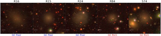
Composite colour cutouts around each UDG from the Subaru / Hyper-Suprime Cam g, r, i-band data. North is up and east is left. The white bar in each image indicates a 5″ scale. Three UDGs, R15, S74 and R84, have central compact sources that are likely galaxy stellar nuclei. We arrange the UDGs, left to right, in order of increasing GC richness. The UDGs S74 and R84 appear to contain additional compact sources and are classified as GC-rich UDGs. Conversely, R15, R16 and R24 appear associated with fewer compact sources and are classified as GC-poor.
2.2 Detailed fitting
To perform more detailed 2D image fitting, we generated 2 × 2 arcmin2 cutout images around each object in both g- and i-bands. These cutouts were large enough to provide sufficient area to reliably estimate the background level. We also generated cutouts of the variance map from hscPipe (Bosch et al. 2018) and used them as the per-pixel flux uncertainties in the fitting. The point spread function (PSF) model of each object was reconstructed for the centre of the cutout based on PSFex results (Bertin 2011). Using SEP (Bertin & Arnouts 1996; Barbary 2016), we detected and masked out all objects on the cutout that were not associated with the UDG’s stellar body. This was challenging for R16 as it is surrounded by a large amount of Galactic cirrus and it was not possible to fully mask some of the very low surface brightness cirrus. S74 is close to a saturated star and a bright background galaxy. For this UDG, we slightly loosened the masking criteria to ensure the main stellar body of S74 was not masked. We experimented with different masking strategies and determined our choice of final masking does not affect the fitting results.
After masking and PSF convolution, we fitted each UDG as a two-dimensional Sérsic function (Sérsic 1968) using the multi-component galaxy image fitting tool Imfit (Erwin 2015,1 similar to e.g. Román & Trujillo 2017; Román et al. 2019, 2021; Kado-Fong et al. 2020; Saifollahi et al. 2021). R15, R84, and S74 all show clear point source-like objects at their centres (Fig. 1) that needed to be modelled simultaneously to the rest of the UDG. We included these nuclei as a two-dimensional Gaussian component in our model. To achieve a robust model, we adopted the Nelder–Mead simplex algorithm for χ2 minimization to avoid any possible local minima found in the fitting process. At the end of each fit, we used the residual image to verify that model adequately accounts for the flux distribution of a UDG. We display an example fit for R15 in Fig. 2.
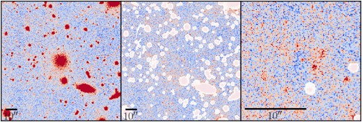
An example of our UDG imfit fitting for R15. Left-hand panel: Our original Hyper Suprime-Cam data. Middle panel: The residuals of our fit with areas masked in the fitting overplotted (white regions). Right-hand panel: A zoom-in at the location of the UDG in the residual image. We plot with ‘asinh’ image stretching in this panel to make the residual structure more evident. For each panel, North is up and East is left. A 10″ bar is also included in each panel.
For low surface brightness galaxies, an incorrect sky background estimate can significantly alter the model (see e.g. appendix C of Pandya et al. 2018). We therefore also tested our sky background model by modelling it as a ‘tilted plane’ with gradients in both X and Y directions. The result of this test indicated that the absence of a background component in our fitting did not affect our final results.
Although the HSC g-band data are used primarily in this work, fitting was performed in all three g, r, i-bands. Fitting in each band was found to be consistent with one another. Furthermore, fitted values obtained from the HST imaging of the UDGs R15, R16 and R84 are in general agreement with the values reported herein. These tests provide additional confidence to the robustness of our fitting process.
The χ2 minimization algorithm does not usually provide meaningful uncertainties of the model parameters when fitting with Imfit. We therefore used the built-in capability of Imfit to perform 1000 bootstrap fitting iterations on images resampled based on the provided noise level. We used these bootstrap fits to estimate uncertainties for our best-fitting results. We summarize the results of our more extensive fitting process, along with associated uncertainties, in Table 1.
A summary of the imaging properties of our Perseus UDG sample. Columns from left to right are as follows: 1) Designation used throughout this work; 2) Right Ascension; 3) Declination; 4) Distance from cluster centre; 5) Semi-major half-light radius (g-band); 6) Average surface brightness within half-light radius (extinction corrected); 7) Axial ratio (g-band); 8) Absolute g-band magnitude (extinction corrected); 9) Stellar mass; 10) g − i band colour (extinction corrected) and 11) GC system richness. For GC system richness, we include the number of GCs used in this work in {curly brackets} after the rich/poor descriptor. For S74 and R24, these are assumed values while the remaining UDGs have preliminary GC richness measurements from the upcoming work of Janssens et al. (in preparation). We note these GC richness measures may be subject to slight revision when published by Janssens et al. (in preparation), however they are unlikely to change from GC-rich to GC-poor (and vice versa). The measurement of photometric properties from HSC imaging is described in Section 2. UDGs that have nuclei and were fitted with a Gaussian + Sérsic profile are indicated with a ‘*’. The remaining UDGs were fitted with a single Sérsic profile. A distance of 75 Mpc for the Perseus cluster is assumed. Absolute magnitudes and surface brightnesses are corrected for g-band Galactic extinction (min 0.495 mag; max 0.685 mag) using Schlafly & Finkbeiner (2011). When relevant, uncertainties are given in (brackets) after values.
| Name | RA | Dec | Rclust | |$R_{\rm e, \mathrm{maj}}$| | 〈μ〉e,g | b/a | Mg | M⋆ | g − i | GC richness |
|---|---|---|---|---|---|---|---|---|---|---|
| PUDG_ | [Deg] | [Deg] | [Mpc] | [″/kpc] | [mag arcsec−2] | [mag] | [×108 M⊙] | [mag] | ||
| R16 | 49.65202 | 41.19229 | 0.51 | 11.6/4.2 (0.06) | 25.70 (0.01) | 0.70 | −15.60 (0.01) | 5.75 | 1.04 | Poor {1} |
| R15* | 49.26584 | 41.24856 | 0.76 | 6.8/2.5 (0.02) | 25.13 (0.02) | 0.97 | −15.35 (0.02) | 2.59 | 0.85 | Poor {1} |
| R24 | 49.64830 | 41.80890 | 0.49 | 9.8/3.6 (0.08) | 24.75 (0.02) | 0.81 | −16.34 (0.01) | 3.91 | 0.68 | Poor {5} |
| R84* | 49.35375 | 41.73929 | 0.66 | 5.6/2.0 (0.01) | 24.98 (0.01) | 0.97 | −15.10 (0.01) | 2.20 | 0.87 | Rich {28} |
| S74* | 49.29835 | 41.16787 | 0.78 | 10.5/3.8 (0.03) | 25.12 (0.02) | 0.86 | −16.19 (0.01) | 7.85 | 0.96 | Rich {30} |
For conversion of distance dependent data, we assume a distance to the Perseus cluster of 75 Mpc (m − M of 34.38). All magnitudes and surface brightnesses are extinction corrected using Schlafly & Finkbeiner (2011) and are quoted in the AB system. We note the maps of Schlafly & Finkbeiner (2011) are significantly coarser than our data and thus a systematic error may be introduced when applying these dust corrections to our data. For g − i colours, we subtract extinction corrected magnitudes from fitting the HSC i-band data from our g-band fits. We calculate stellar masses using UDG luminosities and their g − i colour in the M⋆/Lg relation of Into & Portinari (2013) (i.e. M⋆/Lg min 1.1, max 3.1).
2.3 Sample characteristics
Noting the original UDG definition of van Dokkum et al. (2015) (i.e. μ0,g > 24 mag arcsec−2 and Re > 1.5 kpc) is affected by UDGs with a central nucleus, many literature works instead choose the average surface brightness within the half-light radius (〈μ〉e,g) when defining UDGs (e.g. Yagi et al. 2016; van der Burg et al. 2017; Greco et al. 2018; Janssens et al. 2019). When discussing the UDG criterion in terms of 〈μ〉e,g it is important to also add ∼1 mag to the definition to allow for the larger aperture being probed in order to ensure the galaxies are not brighter than those of the original definition. We therefore adopt a UDG definition of 〈μ〉e,g > 25 mag arcsec−2 and Re > 1.5 kpc in this work.
In Fig. 3, we contextualize our Perseus cluster UDG sample in relation to galaxies from the Coma cluster (Alabi et al. 2020). Under the assumption of Perseus cluster membership (see Section 4 for a confirmation of this) our UDGs are amongst some of the biggest and brightest currently observed. This is a simple selection effect whereby it was necessary to observe the brightest galaxies in order to ensure the data had sufficient S/N to be usable. We note R24 does not formally meet the UDG definition, having a |$\langle \mu \rangle _{e,g}\, \sim$| 0.25 mag too bright. Given its blue colour and visually disturbed morphology, it is likely beginning its infall into the Perseus cluster and will be expected to quench and fade into the UDG regime within ∼0.5 Gyr (see e.g. Román et al. 2021; fig. 4).
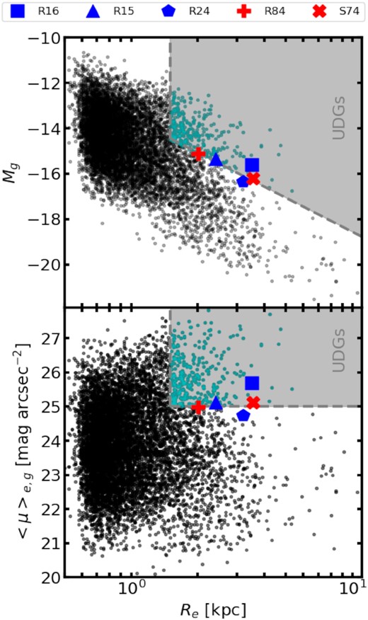
g-band magnitude (top panel) and average surface brightness within half-light radius (bottom panel) versus half-light radius. We plot our Perseus UDGs against the V-band catalogue of Coma cluster galaxies from Alabi et al. (2020) (black points). Galaxies in the Alabi et al. (2020) catalogue meeting the UDG definition are plotted in cyan. The parameter space where UDGs reside has been highlighted by the grey region. Our Perseus sample exists at the borderline of UDG parameter space with magnitudes and surface brightnesses making them amongst the brightest UDGs. R24 is slightly too bright to reside in UDG parameter space but is expected to fade into the UDG regime with quenching.
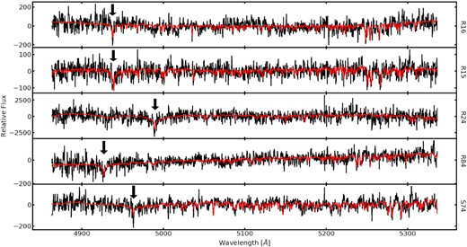
The five KCWI spectra analysed in this work. We plot the final spectra for each UDG (black) along with a representative pPXF fit from our extensive fitting process (red). Perseus UDG names for each spectra are labelled on the right of each panel. In each spectrum we indicate the positioning of Hβ with a black arrow. Based on fits such as these we measure the recessional velocities and velocity dispersions as reported in Table 2.
3 KCWI DATA
3.1 KCWI acquisition
The integral field spectroscopy detailed in this work was acquired using the Keck Cosmic Web Imager (KCWI; Morrissey et al. 2018) during observing runs on the nights 2018 November 12/13, 2018 December 12/13, 2019 October 29/31, 2020 October 20/21, 2020 November 11 and 2020 December 13. We used the medium slicer and the BH3 grating (R ≈ 9750). Observations were largely conducted in dark, clear conditions with good seeing (<1.5″). An exception were the nights of 2020 November 11 and 2020 December 12, where the seeing was poor (>2.5″). We note that we ‘light-bucket’ collapsed our observations of the UDGs so poor seeing is not expected to affect our science results. We also note the nights 2019 October 31, 2019 November 1, 2020 October 20 and 2020 October 21 which had varying levels of high altitude cloud throughout. We found a large decrease in signal-to-noise in our observations of R24 due to this cloud. In order to remove affected frames we visually inspected the whitelight depictions of our data cubes to ensure that R24 was visible, removing those where cloud cover was evident. We then took the remaining frames and coadded in frames in two stages, ensuring each stage increased the signal-to-noise to the final stack and removing those that did not. Of the 20 1200s exposures observed targeting R24, 8 were used in our final stack. We summarize our observations, including observing conditions, program ID and integration times, in Table A1 of Appendix A. Final exposure times were: 25200s for R15, 48600s for R16, 9600s for R24, 25533s for R84 and 20400s for S74.
The data were initially reduced using the KCWI data reduction pipeline (KDERP). Following this we took the non-sky subtracted, differential atmospheric refraction corrected and standard star calibrated ‘ocubes’ and performed the trimming and extra flat fielding steps described in Gannon et al. (2020).
R15 and R84 are sufficiently small that we were able to target the galaxies with the medium slicer and include on-chip sky. Observations of R15 were taken in split configurations, dithering between having sky observed on the CCD above and below the UDG. For sky observed below the UDG, we extract spectra using a 21 × 40 spaxel box centred on the target, taking the rest of the slicer as sky. For sky observed above the UDG, we extracted a 21 × 33 spaxel box centred on the UDG, taking the rest of the slicer as sky. In the case of R84 we extracted a 21 × 24 spaxel box centred on the UDG taking the rest of the slicer as sky.
R16, R24 and S74 are of sufficient size to fill the field of view of the medium slicer and so offset sky observations are used to perform sky subtraction using the technique described in Gannon et al. (2020). Briefly, we use a template for galaxy emission along with an ensemble of offset sky observations to model the non-sky subtracted spectrum and perform sky subtraction. For each of the galaxies, we take the 10 sky frames observed temporally nearest to the science observation being subtracted and use them in this modelling. We note some of these sky exposures may come from other nights or targets during our Perseus observations.
Once the data were sky-subtracted, relevant barycentric corrections were applied (Tollerud 2015) and they were median stacked. The resulting spectra have signal-to-noise per Å of: 15 for R15, 12 for R16, 14 for R24, 16 for S74 and 18 for R84. These signal-to-noise levels are all quoted on the continuum (Table 2).
A summary of the properties of our Perseus UDG sample. Columns from left to right are as follows: 1) Designation used throughout this work; 2) Signal-to-noise ratio on the continuum; 3) UDG recessional velocity; 4) UDG velocity dispersion and 5) Dynamical mass within 3D, circularized half-light radius. Kinematic properties are measured from the KCWI spectra described in Section 3. When relevant, uncertainties are given in (brackets) after values.
| Name | S/N | Vr | σ | M(< R1/2) |
|---|---|---|---|---|
| PUDG_ | [Å−1] | [km s−1] | [km s−1] | [×108 M⊙] |
| R16 | 12 | 4679 (2) | 12 (3) | 4.70 (2.41) |
| R15 | 15 | 4762 (2) | 10 (4) | 2.25 (1.82) |
| R24 | 14 | 7784 (4) | 20 (5) | 11.9 (6.19) |
| R84 | 18 | 4039 (2) | 19 (3) | 6.74 (2.16) |
| S74 | 16 | 6215 (2) | 22 (2) | 16.0 (3.03) |
3.2 Spectral fitting
In order to extract stellar kinematics from our spectra we fitted the spectra using the method described in Gannon et al. (2020) which utilizes the code pPXF (Cappellari 2017). Briefly, the spectrum was fitted with the high resolution Coelho (2014) synthetic spectral library using 241 differing input configurations for pPXF. Fits that reported uncertainties greater than 25 km s−1 in either recessional velocity or velocity dispersion were discarded. Our final reported values were taken from the median of the remaining fits with uncertainties taken from the 1-sigma spread in these values. We provide an example of a fit we deem acceptable for each galaxy in Fig. 4. We consistency-checked our fitting process by splitting the spectra into red and blue halves and fitted these also. Additionally, we performed the same fitting using a KCWI observation of the Milky Way globular cluster M3 as a template.
R84 is the only UDG where the additional regions and template fits did not report recessional velocities within 1 pixel (∼13 km s−1). Here the blue-half of the spectrum reported recessional velocities and velocity dispersions in strong disagreement with the other fitting. We note that this spectrum has noticeably weaker iron absorption features than the other 4 UDGs (Fig. 4) and so fitting in the blue half is dominated by the Hβ line, which poorly constrains the fit on its own. In the fitting of R15 with the M3 template, all three spectral regions (red-half/blue-half/all) yielded higher velocity dispersions than when fitted with the Coelho (2014) library. This was most likely caused by numerical biases that can become present when trying to recover velocity dispersions around the resolution limits of the template(s) being used (Robertson 2017). The velocity dispersion reported by the Coelho (2014) library is below this resolution limit for the M3 template. Final values from the spectral fitting for each of the five galaxies are reported in Table 2.
An additional sky subtraction on S74 was performed using the on-chip ‘sky’. Here we subtracted the fainter outskirts of the galaxy from the central, brighter regions to produce a spectrum and confirm the results of our offset sky subtraction using the Gannon et al. (2020) sky subtraction routine. We stacked the sky subtracted spectra and then fit in the same manner as for the main sample. The final recessional velocity (|$6217\pm 2\, \mathrm{km\ s^{-1}}$|) and velocity dispersion (|$21\pm 3\, \mathrm{km\ s^{-1}}$|) agree well with the values reported for our on chip sky subtraction of S74.
3.3 Dynamical mass
Strictly speaking, to infer dynamical masses we need to measure the luminosity-weighted line-of-sight velocity dispersion within the half-light radius. As our galaxies have half-light radii of ∼6″ to 11″, their effective diameters are well matched to the size of KCWI’s medium slicer (∼16″ × 20″). Our velocity dispersions will therefore be approximately luminosity-weighted within the half-light radius.
We caution that there exists evidence that the Wolf et al. (2010) formula may become biased in the case of dispersion supported systems undergoing tidal disruption (Errani, Peñarrubia & Walker 2018; Carleton et al. 2019). R24 displays a non-smooth stellar body (see Fig. 1) which suggests it may be undergoing a tidal interaction and thus have a biased mass estimate from equation (1). In principle, this might affect our other Perseus UDGs as tidal features (if present) are likely below the surface brightness limit of our data due to their fast diffusion times (Peñarrubia, Navarro & McConnachie 2008; Carleton et al. 2019). We note however, the work of Doppel et al. (2021) who suggest biases due to tidal effects are short lived in dwarf galaxies after pericentric passages.
4 DISCUSSION
4.1 Confirmation of UDG status
In Fig. 5, we plot the positions on the sky of our Perseus UDGs, along with galaxies from the 2M++ sample of relatively bright galaxies (Lavaux & Hudson 2011) that are in the direction of the Perseus cluster. All of our UDGs have recessional velocities within 2.5σ of the mean recessional velocity of the Perseus cluster. Additionally, all of our UDGs are well within 0.2 – 0.4 R200 (projected) of the Perseus cluster. It is therefore highly likely that all of our Perseus UDGs are cluster members (see Fig. 6 for an alternate visualization of this). This environmental association is fully consistent with our assumption of a 75 Mpc distance for our Perseus UDGs. This distance formalizes their large half-light radii (Re > 1.5 kpc). Combining this with the surface brightness measurements in Section 2 and Table 1 we confirm the status of our sample as four ‘bona fide’ Perseus UDGs and one galaxy, R24, which is likely soon to fade into the UDG regime.
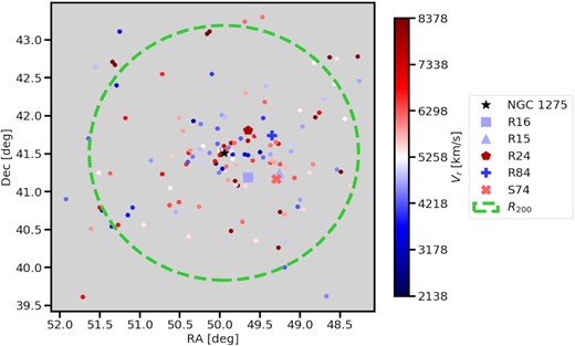
UDG positioning within the Perseus cluster. We plot our UDGs (R15 - triangle, R16 - square, R25 - pentagon, S74 - cross and R84 - plus) along with other, brighter galaxies in the direction of the Perseus cluster from the 2M++ sample of Lavaux & Hudson (2011) (circles). We include the central, bright cluster galaxy NGC 1275 as a reference (black star). We colour code points by their difference from the mean recessional velocity of the Perseus cluster. Our colour scheme is set to have upper and lower limits of 3 times the Perseus galaxy velocity dispersion about the mean recessional velocity of the cluster. A green circle is included to represent the virial radius of the cluster. All UDGs are projected to be well within the cluster limits.
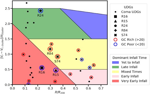
A phase space diagram of the Perseus and Coma cluster UDGs. We plot the absolute difference of the galaxy recessional velocity from the mean of the cluster, normalized by the cluster velocity dispersion versus projected radius from cluster centre (normalised by the virial radius of the cluster). We plot our Perseus UDGs (triangle, square, pentagon, cross and plus) along with UDGs in the Coma cluster (Alabi et al. 2018 and Yagi358 from Gannon et al. in preparation). UDGs hosting GC systems measured in excess of 20 GCs are deemed GC-rich (circled in red). UDGs hosting GC systems with fewer than 20 GCs are deemed GC-poor (circled in blue). Coma UDG GC system estimates are from Forbes et al. (2020) and references therein. Perseus GC richness categories are as designated by this work. We overlay regions from the simulations of Rhee et al. (2017) to aid in our interpretation of the UDGs (red/pink/yellow/green/blue regions). We note our phase space diagram is in 2D, projected space and that the 3D radius and/or velocity for objects may be much larger. Our Perseus UDG sample appears well bound to the cluster. It is more likely that our Perseus GC-poor UDGs have undergone cluster infall at earlier times than their GC-rich counterparts. This effect is diluted when adding in the Coma cluster to our analysis.
4.2 UDG infall times
In Fig. 6, we plot the difference in galaxy recessional velocity with the mean of the cluster normalized by the cluster’s velocity dispersion versus the projected radius from the centre of the cluster in units of cluster virial radii. We supplement our Perseus UDG sample with UDGs from the Coma Cluster (Alabi et al. 2018 and the UDG Yagi358, Vr = 7967 km s−1, from Gannon et al. in preparation; Yagi et al. 2016). For the Coma cluster UDGs we colour code them according to their measured GC system richness from Forbes et al. (2020) and references therein. For our Perseus UDGs we similarly colour code them on the basis of their identified GC richness class.
In order to quantify the likely infall timescales of the UDGs we over-plot the phase-space regions derived from galaxies located in 16 clusters within the cosmological, hydrodynamic simulations of Rhee et al. (2017). These regions represent the different time periods in which galaxies have most likely fallen into the cluster and are designed for easy comparison to observations. We note Fig. 6 of Aguerri et al. (2020) provides empirical observational evidence that other Perseus galaxies are broadly consistent with the Rhee et al. (2017) predictions. We summarize the expected fractions of galaxy infall times in each region based on the simulations of Rhee et al. (2017) in Table 3.
Fractions of galaxies in each infall time period for the coloured regions of Fig. 6 from the simulations of Rhee et al. (2017) (rounded to 2 decimals). Regions are named corresponding to their dominant population of galaxies. ‘PI’ is an acronym for ‘pre-infall’. Interlopers are galaxies that are non-members of the cluster despite projection effects placing them within projected cluster phase space.
| Infall region | Infall time period [Gyr] | ||||
|---|---|---|---|---|---|
| PI | 0< | 3.63< | 6.45< | Interloper | |
| <3.63 | <6.45 | <13.7 | |||
| Yet to | 0.35 | 0.04 | 0.05 | 0.01 | 0.54 |
| Late | 0.02 | 0.37 | 0.15 | 0.31 | 0.14 |
| Mixed times | 0.13 | 0.32 | 0.20 | 0.23 | 0.12 |
| Early | 0.18 | 0.20 | 0.27 | 0.17 | 0.19 |
| Very early | 0.03 | 0.17 | 0.22 | 0.52 | 0.06 |
For example, the red region plotted in Fig. 6 is dominated by galaxies that have fallen into the cluster at the earliest times. More specifically |${\sim}52{{\ \rm per\ cent}}$| of galaxies found in this region are expected to have infall times >6.45 Gyr ago. Of the remaining galaxies, we expect |${\sim}22{{\ \rm per\ cent}}$| to have infall times between 3.63 and 6.45 Gyr and |${\sim}17 {{\ \rm per\ cent}}$| to have only recently fallen into the cluster (<3.63 Gyr ago). The remaining, ‘interloper’, galaxies are not located in the cluster despite projection effects placing them within cluster phase space.
The UDGs in our Perseus sample all have phase-space locations consistent with them being bound to the Perseus cluster. An exception may be R24 which is located in the green region of Fig. 6. This suggests that if it is not infalling for the first time it is probable that it will fall in soon. Of interest for the other four UDGs is the difference between the two GC-rich and two GC-poor UDGs.
Our data suggest that the GC-poor UDGs (R15 and R16) are more likely to have fallen into the cluster at earlier times than the GC-rich UDGs (S74 and R84). However, we caution that we are dealing with small number statistics and that, even within the regions from the simulations of Rhee et al. (2017), there are significant variations in the infall times of individual galaxies. The observed trend largely disappears after the inclusion of data from the Coma cluster.
Formation scenarios where GC-rich UDGs form preferentially at high-redshift and quench early (e.g. Carleton et al. 2021) logically require the early accretion of GC-rich UDGs to the cluster for the quenching to be environmentally driven. Objects accreted to the cluster at early times are expected to have smaller relative velocities and orbital radii which reflect the smaller gravitational potential at the time of accretion (see further Rhee et al. 2017). Therefore, if GC-rich UDGs are environmentally quenched at high redshift we have an expectation that they will inhabit the more bound regions (red/pink) of Fig. 6.
Conversely, GC-poor UDGs are expected to have formation pathways and dark matter halo masses similar to field low surface brightness dwarfs (e.g. Beasley & Trujillo 2016). Due to this they cannot survive long in the strong tidal fields of the cluster core and are expected to predominantly inhabit the later earlier infall times regions of Fig. 6 (blue, green, yellow). We therefore expect a trend between UDG infall time and UDG GC system richness where GC-Rich UDGs infall at earlier times.
The lack of this trend in Fig. 6 suggests that GC-rich UDG quenching is not environmentally driven. Furthermore, the axial alignment of UDGs at radii >0.5R200 of the cluster Abell 2634 suggests that they have experienced little evolution in the cluster thus far (Rong et al. 2020). If UDG quenching is not environmentally driven it may be either self induced or triggered via pre-processing of GC-rich UDGs in a group environment. We note, it has already been observed for some UDGs that quenching episodes can precede their cluster infall (e.g. M-161-1 Papastergis, Adams & Romanowsky 2017; Dragonfly 44 Alabi et al. 2018) implying environmental processes are not the only driver of their evolution. Further constraints on these mechanisms can be added through the analysis of their star formation histories (see further Ferré-Mateu et al. 2018). For our Perseus UDGs this will be presented in another paper (Ferré-Mateu, in preparation).
4.3 Perseus UDG halo masses
In Fig. 7, we compare the dynamical mass measurements for our Perseus UDGs to cuspy, NFW dark matter haloes (Navarro et al. 1996) and cored dark matter haloes (Di Cintio et al. 2014). We include four literature UDGs with stellar kinematics and GC counts (van Dokkum et al. 2017, 2019b; Gannon et al. 2020; Forbes et al. 2021). All are GC rich. When considering the four Perseus galaxies that currently meet the UDG criterion (i.e. not R24) along with the literature UDGs, we find that UDGs with a rich GC system have greater dynamical mass within their 3D half-light radius. This agrees with a first order interpretation of GC-rich UDGs residing in higher mass dark matter haloes.
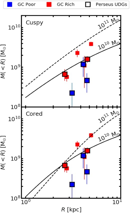
Enclosed mass versus galactocentric radius. We plot the dynamical mass measurements from stellar kinematics for our Perseus UDGs (black outline) along with those from the literature (van Dokkum et al. 2017, 2019b; Gannon et al. 2020; Forbes et al. 2021). UDGs are colour coded by GC richness with red points GC-rich and blue GC-poor. Top panel: we compare to cuspy, NFW (Navarro, Frenk & White 1996) haloes of mass 1 × 10¹⁰ M⊙ (solid line) and 1 × 10¹¹ M⊙ (dashed line). Bottom panel: we compare to cored (Di Cintio et al. 2014) haloes of mass 1 × 10¹⁰ M⊙ (solid line) and 1 × 10¹¹ M⊙ (dashed line). Overall, GC-rich UDGs have higher dynamical masses than those that are GC-poor. When trying to connect this to their total halo mass the interpretation is more complex (see text for details).
Due to our small sample of UDGs, we ran simulations to see how often we expect this trend to arise via random chance. For each simulation, we randomly assigned either a high dynamical mass or low dynamical mass to the nine UDGs (5 Perseus + 4 literature) with equal probability. We ran 10 000 simulations. In only 78 simulations of the 10 000 (0.78 per cent) did we observe the trend seen in Fig. 7. Namely, in these simulations we observe all GC-rich UDGs to have high dynamical masses while two of three GC-poor UDGs had low dynamical masses. If we exclude the GC-poor UDG with high dynamical mass, R24, which both does not currently fit the UDG criteria and may not be in dynamic equilibrium, only 47 of our 10 000 simulations (0.47 per cent) match the trends seen in Fig. 7. We conclude it is highly unlikely that our observation of GC-rich UDGs having higher dynamical masses than GC-poor UDGs has arisen based on random fluctuations alone.
When taking into account the effect of extrapolating dynamical masses into total halo masses using halo profiles, the interpretation of Fig. 7 becomes more complex. Greater dynamical mass implying greater total halo mass is only generally true under the assumption of cuspy dark matter haloes for UDGs with fixed halo parameters (e.g. concentration parameters drawn from the same relation such as Dutton & Macciò 2014). Unfortunately, it is likely misleading to compare UDG dynamical masses to cuspy dark matter halo profiles. There is evidence that favours cored halo profiles for UDGs in simulations (Di Cintio et al. 2017; Carleton et al. 2019; Martin et al. 2019) and observations (van Dokkum et al. 2019b; Wasserman et al. 2019; Gannon et al. 2020).
In the case of cored haloes, lone dynamical masses at a single radius poorly constrain the total halo mass of the UDG (see further Gannon et al. 2021). For example, it is clear that our dynamical mass measurement for R84 agrees well with cored haloes of both mass 1010 M⊙ and 1011 M⊙ and so cannot constrain the total halo mass of the UDG (Fig. 7, bottom panel). Thus, when assuming a cored dark matter halo profile our measurement of greater dark matter mass within the central region implies little more than that GC-rich UDGs have greater dark matter mass in their centres. For example, it is possible that they reside in dark matter haloes of the same total mass as GC-poor UDGs, but the GC-poor UDGs are more efficient at creating a core and therefore have less mass in the halo centre.
We are therefore able to draw two possible conclusions from Fig. 7: 1) GC-rich UDGs reside in haloes of greater total mass than GC-poor UDGs, as expected given the GC number – halo mass relation of Burkert & Forbes (2020), or 2) GC-rich UDGs reside in haloes of a similar mass to GC-poor UDGs but with a different halo profile. In order to have the same total mass the halo profile must be more concentrated and with higher central dark matter densities. This implies the total dark matter halo is of smaller radius due to the increase in its density. We note option 2) would align with halo concentration predictions for GC-rich UDGs from Trujillo-Gomez, Kruijssen & Reina-Campos (2021) although it is unclear how they are able to reproduce the observed breadth in UDG dynamical masses.
4.4 Trends with GC system richness
In Fig. 8 we plot our observations for R15, R16 and R84, supplemented by UDGs from the literature (Beasley et al. 2016; van Dokkum et al. 2017, 2019b; Cohen et al. 2018; Gannon et al. 2020; Forbes et al. 2021; Müller et al. 2021). R15 and R16 are plotted as having 1 GC as their selected GC counts are consistent with background levels. We also include the Perseus UDGs R24 and S74 that do not have exact NGC measurements by assuming a GC count based on their visually identified class of GC richness as per Section 2.1. For R24, we assume five GCs to place it in a representative position within the GC-poor class. For S74, we assume 30 GCs to place it at a similar level of GC richness to R84.
GC number, a known halo mass indicator for normal galaxies, versus half-light radius (left-hand panel), stellar velocity dispersion (centre panel) and dynamical mass (right-hand panel). We include a second y-axis of total dark matter halo masses using the NGC – MHalo of Burkert & Forbes (2020). We plot the three Perseus UDGs with approximate GC numbers (R15, R16 and R84) from Janssens et al. (in preparation) along with a sample of UDGs from the literature (orange squares; Beasley et al. 2016; van Dokkum et al. 2017, 2018a, 2019a,b; Cohen et al. 2018; Gannon et al. 2020; Forbes et al. 2021; Müller et al. 2021). We add to this sample our two Perseus UDGs without a NGC measurement by assuming a roughly expected GC number. We also plot UDGs from the simulations of Carleton et al. (2021, black points). Labels are included for regions of GC richness as prescribed by this work and separated by horizontal dashed lines. ‘GC-poor’ systems indicate low total halo masses and likely correspond to ‘Puffy Dwarf’ UDGs. ‘GC-rich’ systems indicate high total halo masses and likely correspond to ‘Failed Galaxy’ UDGs. The plot is labelled appropriately for both. Clear observational trends are apparent for UDG GC system richness with both dynamical mass and stellar velocity dispersion.
Literature UDG properties, barring GC counts, are from appendix A of Gannon et al. (2021) and the references therein. For the Virgo cluster UDG VCC 1287 we use the GC system counts of Beasley et al. (2016; NGC = 22 ± 8). For the Coma Cluster UDGs Dragonfly 44 (NGC = 74 ± 182) and DFX1 (NGC = 62 ± 17) we use the measurements of van Dokkum et al. (2017). For the NGC 5846 group UDG NGC 5846_UDG1 (NGC = 37 ± 5) we use the GC system measurement of Müller et al. (2021).3
The literature sample of UDGs in Gannon et al. (2021) also includes the UDGs NGC 1052_DF2 and NGC 1052_DF4 which have had their GC systems measured. Shen et al. (2021) find evidence that many of the GCs orbiting the NGC 1052 UDGs are actually ultra-compact dwarfs due to their luminosity. The GC systems of both UDGs comprise ∼19 star clusters but it is not obvious how these compare to the other UDGs plotted due to their markedly different luminosity function (Shen et al. 2021). We therefore choose to exclude them when adding the sample of Gannon et al. (2021) literature UDGs to Fig. 8.
We now compare these observed galaxies to the simulated UDGs of Carleton et al. (2021). They used a semi-analytic model combined with the Illustris-TNG simulation to form GC-rich UDGs in clusters of M200 ≥ 2 × 10¹⁴ M⊙. The authors do not quote maximum cluster mass is in the simulation. Carleton et al. (2021) suggests the primary cause of UDG formation in clusters is rapid star formation at high redshift combined with prolonged tidal heating within the cluster’s gravitational well. For more details on the UDG formation simulation and the model applied for GC formation see Carleton et al. (2019), Carleton et al. (2021).
Under the Carleton et al. (2021) simulated UDG formation model there is the expectation that GC number should correlate with half-light radius. However, in the observed UDGs there is no clear trend in GC number – half-light radius parameter space (Fig. 8, left-hand panel; Pearson’s r = 0.16). The three GC-poor UDGs plotted are from our Perseus sample which is selected to have approximately equivalent half-light radii between GC-rich and GC-poor UDGs. Our observational data is therefore insufficient to comment on the actual trend in half-light radius with GC number. We note that due to the relatively small spread in luminosities for those UDGs with GC number measurements, Forbes et al. (2020) Fig. 7 provides evidence of a weak inverse trend in this relationship for Coma cluster UDGs. This would be the opposite of the expectation from Carleton et al. (2021)’s simulations.
Based on the observed NGC – MHalo relation of Burkert & Forbes (2020) there is a first order expectation that GC number should correlate with dynamical mass. For pressure-supported systems it is well established dynamical mass is proportional to the half-light radius and the square of the velocity dispersion (e.g. Wolf et al. 2010; Errani et al. 2018). We have established that our data are not sufficient to reveal trends with half-light radius. Interestingly, there does seem to be a correlation between GC number and velocity dispersion (Fig. 8, middle panel; Pearson’s r = 0.91). This suggests UDGs with more GCs are dynamically ‘hotter’. The same trend is not apparent in Carleton et al. (2021) simulated UDGs with many GC-poor UDGs having similar velocity dispersions to GC-rich UDGs.
To first order, we expect GC number to correlate with dynamical mass given they correlate with halo mass. Namely, we expect ‘failed galaxy’ UDGs to have higher dynamical masses due to their more massive dark matter halo. Similarly, we expect ‘puffy dwarf’ UDGs to have smaller dynamical masses indicative of their dwarf-like dark matter halo. We observe this observational trend, between GC number and dynamical mass (Fig. 8, right-hand panel; Pearson’s r = 0.85), although it may be slightly diluted by our choice to half-light radius match in the Perseus sample. A similar trend also appears in the Carleton et al. (2021) simulated UDGs. This is slightly puzzling due to the lack of trend between velocity dispersion and GC number in their simulation.
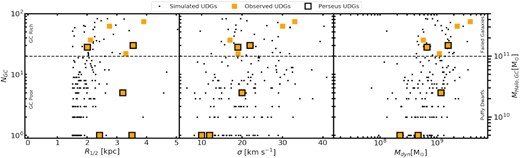
In Fig. 9, we investigate the Carleton et al. (2021) simulations further. Here, we compare their simulated galaxies’ halo masses and GC numbers to the observationally established NGC – MHalo of Burkert & Forbes (2020). It is clear neither the simulated UDGs, or the simulated non-UDGs, follow the observational relationship. This is particularly true when considering the tight scatter of the NGC – MHalo once a GC system becomes large enough to mitigate statistical effects (≳20). Particularly troubling are those galaxies hosting large GC systems similar to the Milky Way (i.e. ≳150) but halo masses of order 109 M⊙. Likewise, there appear to be galaxies of large halo mass (i.e. ≳1011 M⊙) but with only one or two GCs.
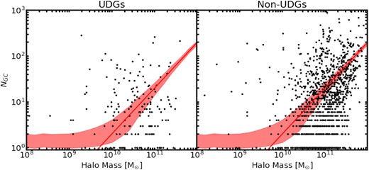
Globular cluster number versus halo mass. We plot Carleton et al. (2021) simulated UDGs (black points; left) and the simulated data for a stellar mass matched sample of non-UDG galaxies in the UDG stellar mass range (black points; right). We include the observationally established relation of Burkert & Forbes (2020) (red line) for non-UDGs with indicative scatter (red fill). The simulations of Carleton et al. (2021) do not reproduce the observed NGC – MHalo relationship even for non-UDGs.
Current theory suggests the NGC – MHalo relation should be established at z ≳ 6 (Boylan-Kolchin 2017). Our investigations showed the Carleton et al. (2021) simulations do not follow the relationship at cluster infall either, when the NGC – MHalo relationship should already be established. We suggest future simulations seeking to simulate the GC systems of UDGs must, as a basic requirement, seek to reproduce the Burkert & Forbes (2020) relationship for non-UDGs.
5 CONCLUSIONS
In this work we study five UDGs residing in the Perseus cluster using HSC imaging and KCWI spectroscopy. We find two of them likely harbour GC-rich populations and three have GC-poor populations. Our main conclusions from this study are as follows:
Our KCWI spectroscopy confirms Perseus cluster membership and, along with our HSC imaging, confirms four of our sample of galaxies meet the UDG criteria. The exception is R24 which is slightly brighter than the standard UDG definition. We find this galaxy is likely infalling into the Perseus cluster for the first time and, after quenching, is expected to fade into the UDG regime within ∼0.5 Gyr.
By measuring a stellar velocity dispersion we calculate dynamical masses within half-light radii for our sample. After supplementing our sample with literature UDGs we find UDGs with richer GC systems have greater dynamical mass within the half-light radius. They also have larger velocity dispersions. This is as expected by a first order interpretation that GC-rich UDGs reside in more massive dark matter haloes. However, we stress that this does not necessarily indicate GC-rich UDGs are in more massive haloes. Extrapolation of dynamical masses into total halo masses requires the non-trivial assumption of a dark matter halo profile. A difference in the nature of their halo profiles (e.g. GC-poor UDGs exhibiting a stronger dark matter core) may also explain the difference in central dark matter mass.
No clear correlation exists between GC system richness and phase space positioning in the cluster. This is in contrast to the expectations of high-redshift GC-rich UDG formation scenarios where they are predicted to environmentally quench within clusters at early times. Either internal mechanisms or pre-processing in groups may instead be required to explain the known quenching of UDGs.
No clear correlation exists between UDG GC numbers and host galaxy half-light radii. This is likely due to the lack of an unbiased sample of GC poor UDGs. Our observed GC poor UDGs were selected to have similar sizes to GC rich UDGs.
ACKNOWLEDGEMENTS
We thank the anonymous referee for their insightful comments which greatly helped improve the quality of the work. We thank A. Alabi and T. Carleton for kindly providing their data for use in Section 4. JSG and AJR wish to thank A. Alabi for doing preliminary analyses data relating to this work. JSG acknowledges financial support received through a Swinburne University Postgraduate Research Award throughout the creation of this work. AFM has received financial support through the Postdoctoral Junior Leader Fellowship Programme from ‘La Caixa’ Banking Foundation (LCF/BQ/LI18/11630007). AJR was supported by National Science Foundation Grant AST-1616710 and as a Research Corporation for Science Advancement Cottrell Scholar. Support for Program number HST-GO-15235 was provided through a grant from the STScI under NASA contract NAS5-26555.
The data presented herein were obtained at the W. M. Keck Observatory, which is operated as a scientific partnership among the California Institute of Technology, the University of California and the National Aeronautics and Space Administration. The Observatory was made possible by the generous financial support of the W. M. Keck Foundation. The authors wish to recognize and acknowledge the very significant cultural role and reverence that the summit of Maunakea has always had within the indigenous Hawaiian community. We are most fortunate to have the opportunity to conduct observations from this mountain.
This paper is based [in part] on data from the Hyper Suprime-Cam Legacy Archive (HSCLA), which is operated by the Subaru Telescope. The original data in HSCLA was collected at the Subaru Telescope and retrieved from the HSC data archive system, which is operated by Subaru Telescope and Astronomy Data Center at National Astronomical Observatory of Japan. This paper makes use of software developed for the Vera C. Rubin Observatory. We thank the observatory for making their code available as free software at http://dm.lsst.org.
DATA AVAILABILITY
The KCWI data presented are available via the Keck Observatory Archive (KOA): https://www2.keck.hawaii.edu/koa/public/koa.php 18 months after observations are taken. The HSC data presented herein will be shared upon reasonable request with the corresponding author.
Footnotes
Although see Saifollahi et al. (2021) for an alternative view of the GC system richness of Dragonfly 44.
Müller et al. (2021) refers to this UDG as MATLAS-2019.
REFERENCES
APPENDIX A: KCWI OBSERVATIONS SUMMARY
In the following table, we summarize the observing conditions and integration times of the KCWI observations used in this work.
A summary of the KCWI data observed whose analysis comprises part of this work. ‘Science’ observations are those targeting the UDG. ‘Sky’ observations are those targeting offset sky positions.
| UDG | Program ID | Night | Conditions | Target | Integration time |
|---|---|---|---|---|---|
| PUDG_R15 | U216 | 2019 Oct 29 | Clear | Science | 16 × 1200s |
| Sky | 6 × 1200s | ||||
| U216 | 2019 Oct 31 | Sporadic cloud | Science | 5 × 1200s | |
| Sky | 2 × 1200s | ||||
| PUDG_R16 | U107 | 2018 Nov 12 | Clear | Science | 6 × 1200s |
| Sky | 1 × 1200s, 1 × 600s | ||||
| U107 | 2018 Nov 13 | Clear | Science | 13 × 1200s | |
| Sky | 3 × 1200s, 1 × 900s | ||||
| U107 | 2018 Dec 12 | Clear | Science | 9 × 1200s | |
| Sky | 2 × 1200s, 1 × 720s | ||||
| U107 | 2018 Dec 13 | Clear | Science | 3 × 1800s, 2 × 1200s | |
| Sky | 1 × 1200s | ||||
| U216 | 2019 Oct 31 | Sporadic cloud | Science | 6 × 1200s | |
| Sky | 2 × 1200s | ||||
| PUDG_R24 | W140 | 2020 Oct 20 | Strong cloud | Science | 11 × 1200s |
| Sky | 5 × 1200s, 1 × 900s | ||||
| U088 | 2020 Oct 21 | Mild cloud | Science | 9 × 1200s | |
| Sky | 4 × 1200s, 1 × 600s | ||||
| PUDG_R84 | U088 | 2020 Nov 11 | Poor seeing, clear | Science | 8 × 1200s, 1 × 813s |
| U088 | 2020 Dec 13 | Poor seeing, clear | Science | 12 × 1200s, 1 × 720s | |
| PUDG_S74 | U216 | 2019 Nov 1 | Sporadic cloud | Science | 17 × 1200s |
| Sky | 5 × 1200s |
